
Abstract
Using perception data to excavate vehicle travel information has been a popular area of study. In order to learn the vehicle travel characteristics in the city of Ruian, we developed a common methodology for structuring travelers’ complete information using the travel time threshold to recognize a single trip based on the automatic license plate reader data and built a trajectory reconstruction model integrated into the technique for order preference by similarity to an ideal solution and depth-first search to manage the vehicles’ incomplete records phenomenon. In order to increase the practicability of the model, we introduced two speed indicators associated with actual data and verified the model’s reliability through experiments. Our results show that the method would be affected by the number of missing records. The model and results of this work will allow us to further study vehicles’ commuting characteristics and explore hot trajectories.
Keywords
Introduction
The mobile trajectory can be defined as the path generated by the moving entity in space, Spaccapietra et al. 1 had defined “trajectory” with “space-time path,” which is recognized by other scholars.2–4 With the rapid development of location tracking and storage technology, people have been able to collect a large number of vehicle and human mobile trajectory data (abbreviated trajectory data), the analysis of trajectory data can effectively help people understand the traffic conditions of a city and the law of people’s movement. Trajectory data contain both space and time attributes, large data volume, and high dimensions; now, the relevant researches mainly include evaluation and prediction of the road network state,5–9 mining individual travel characteristics, 10 inferring the home/work locations,11–16 the commuting characteristic analysis, 17 and so on.
However, most trajectory data from these researches were acquired from the mobile traffic sensors, including data from the Global Positioning System (GPS),18–21 smart phones,22,23 and smart cards.24–26 There are also trajectory data from fixed sensors, called the automatic license plate reader (ALPR) data. Through advanced optoelectronic, computer, image processing, pattern recognition, and remote data access technologies, intelligent ALPR systems achieve the all-weather real-time monitoring of motor vehicle and bicycle lanes in the monitored sections; with the analysis of captured images, front-end processing systems automatically obtain the vehicles’ recorded time when they pass by the test point, as well as their location, direction, plate number, plate color, body color, and other data, and this information is then transferred to the database of the ALPR system control center for data storage, query, comparison, and processing by the computer network (Figure 1).

Intelligent ALPR system structure.
Different from the trajectory data above, the ALPR data were easy to acquire and have a rich data format; currently, the equipment has been installed and used in many cities of China. While these ALPR data have been widely used in violation accident monitoring, their utilization rate is still not very high, leading to a high necessity to mine ALPR data in vehicle trajectory reconstruction.
However, the ALPR data also have some flaws, due to the limitations of license plate recognition technology;27,28 the equipment that were installed in vehicle and roadside are affected by environment and the performance of sensors. The incomplete and abnormal deviation of trajectories is obtained. Using these unhandled data would impact the accuracy and reliability of the results. Therefore, it is significant to reconstruct the missing vehicle trajectories.
There are already some trajectory reconstruction methods29–31 for mobile sensors data, while most methods do not take the actual road network and the validation with measured data into account.
Based on the research situation, this article will propose trajectory reconstruction method combining traffic characteristics to solve the vehicle trajectory missing, and we would use the ALPR data to verify this method.
The rest of this article is organized as follows: section “Data description and preprocessing” summarizes the existing trajectory reconstruction methods. Then, we introduce the data source and some preprocessing approaches. Section “The trajectory reconstruction model” proposes the reconstruction model and parameter calculation. Section “Empirical validation of the model” presents the numerical experiment results based on the empirical ALPR data. Conclusions and future research directions are discussed in section “Concluding remarks.”
Literature review
For the problem of trajectory data missing, we summarized the existing solutions and divided them into three categories:
The first category does not consider the missing ALPR data,18,32,33 but this may cause large errors when missing many samples.
The second category is to fix the lost data separately combined with specific analysis. For example, Castillo et al. 34 proposed a traffic flow prediction method based on Bayesian networks, which could effectively reduce the omission of or errors in license plate recognition. However, this method is only suitable for adjacent road sections in a small-scale city network.
The third is the reconstruction of vehicle trajectory, a more extensive method of interpolation. Through the effective interpolation algorithm, we track and restore the space–time trajectory. The current interpolation method mainly adopts linear interpolation algorithm.
Frentzos et al. 35 proposed query processing algorithms to perform nearest neighbor (NN) search on R-tree-like structures 36 storing historical information about moving objects. Although this linear interpolation algorithm could solve some trajectory reconstruction problems, in practice, even if the vehicle runs on a straight road, its trajectory would not be completely straight.
Kim et al. 37 described an iterative refinement method for approximating a cubic B-spline interpolation of unit quaternions to construct the curve trajectory; however, the calculation procedure is complex and just for some special curves.
Yu and Kim 38 used the high-order polynomial to interpolate the curve, but Loan 39 proved that the high-order polynomial tends to cause the vibration of the curve, and the convergence of interpolation is not good. Yu et al. 40 proved that using curves to indicate the space–time trajectory of moving objects is more accurate than line segment, and proposed a piecewise polynomial method to interpolate trajectory, these require quantity and thus is not suitable for high-dimension expansion.
All these studies represent a moving trajectory as a sequence of connected segments in space–time, and each segment has two end points that are consecutively reported factual states.
There is another method 41 treating vehicle travel as a consequence of the choice of different routes. Wang et al. created a direct access network model, based on which constructed the track patching set, and finally made optimal decision to the track patching set using track utility function. However, the assumption is not verified using large-scale real-life data.
This article proposes a trajectory reconstruction method for the ALPR data, which does not need microscopic representation of vehicle running trajectory; the model is simple and convenient to calculate. And we demonstrated its scalability and efficiency through an extensive experimental study using large synthetic and real datasets.
Data description and preprocessing
Data description
We utilized the vehicle identification data of Ruian, Zhejiang province, China, where ALPR facilities have been installed in 108 intersections. Figure 2 shows the distribution of the 108 data collection points, and all of the 108 intersections data have been used in calibration and validation in this article. These detectors cover the major roads in Ruian seen on the map, and the data clearly reflect the vehicles’ running state. The database receives millions of records every day. In total, two data collection periods are used in this study: one between 29 December 2015, 00:00:00 and 4 January 2016, 23:59:59, and another between 1 March 2016, 00:00:00 and 21 March 2016, 23:59:59.

The distribution of the detectors.
Data preprocessing
There were 20 working days and 8 testing days in the two datasets. We used SQL server to finish the data preprocessing. After importing the data into the database and storing them in a table named “dbo.source,” we selected useful columns from the original 38 fields. The filtered dataset format is shown in Table 1.
Summary of the datasets.

Due to the limitations of the image recognition technology, some vehicles’ plate numbers could not be clearly captured, so it was necessary to remove these unidentified records from our datasets. These records were dropped by an execute statement: “delete from dbo.source where HPHM like ‘identified.’” Finally, we deleted approximately 10% of the data. Since there was a red light in the intersections, some of the uploaded data from certain facilities were repeated. As a result, there were many duplicate records that needed to be removed from the datasets. Our approach for recognizing duplicate records included the following steps:
The same records include the same time.
In total, two adjacent records are the same except for the time, and the time interval of two records is less than threshold A.
We found that threshold A depends on the all red time of the intersection, and the vehicle stopped for the all red light and was detected repeatedly at the same location; here, we assumed A = 5 s, which would represent the all red time in this article.
Vehicle trip extraction
In the process of mining, the vehicle travel information is based on the ALPR data; it is imperative to obtain complete vehicle travel trajectories, so this section organizes the data according to the vehicle itself and identifies the vehicle’s single trip through the travel time threshold. We include a vehicle trajectory reconstruction model with the technique for order preference by similarity to an ideal solution (TOPSIS) algorithm, 42 which effectively completes the vehicle travel information based on the ALPR data. We then show the complete single vehicle trip information. The reliability of our model was demonstrated by experiments.
Data organization
Before we mined the travel information of each vehicle, we first constructed the individual vehicle’s travel portfolio: a list of complete records, ranked by the time. All these records were connected to a series of integral travel trajectories. All research in this article were based on the individual vehicle’s travel information. Faced with an enormous amount of data, we first divided the data by the record time. We then grouped these records according to license plate number.
Single-vehicle trip recognition
The record for a vehicle contained multiple single trips in 1 day. We segmented all the single trips of each vehicle using the travel time threshold B every day. We defined the single trip as meeting the condition that the time interval between the current trip and adjoining trips exceed B. We obtained the time interval by computing the time gap of two consecutive records. If the time gap was larger than B, we distinguished the two records into two different trips. We were able to obtain a vehicle’s travel information and determined the value of B using formula (1)

where
The trajectory reconstruction model
In this section, we proposed a method to solve vehicle trajectory missing for the ALPR data. According to original data and actual road network, we found all incomplete vehicle trajectory records and used depth-first search (DFS) 43 to find all possible routes and finally solved the trajectory decomposition set decision with TOPSIS and achieved trajectory reconstruction (Figure 3).

The trajectory reconstruction method flowchart.
The first step is to determine the research area; to facilitate the understanding of the model, we created a simple road network (Figure 4(a)) consisting of 16 nodes, 12 links, and we assumed that all the road sections are of the same nature, and the length of the section, road direction, and other network information are known.
We projected a vehicle’s travel data into the road network, which cannot form a complete route; this means that there is no direct link between some adjacent two records. This issue belongs to the vehicle trajectory missing, as shown in Figure 4(b), and the vehicle trajectory records (node 1, node 2, node 7, node 11, node 12, and node 16) are projected into the road network; it was first tested at locations 1 and 2 and then tested again at locations 7, 11, 12, and 16 apparently, and there were some missing records.
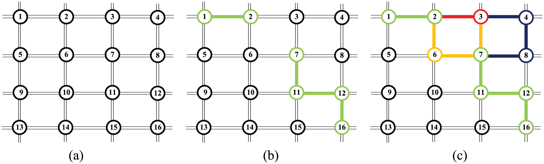
Road network and incomplete vehicle trajectory: (a) is the road network and black circles with numbers are the detection locations, green circles in, (b) are the known vehicle trajectory records, the yellow, red and blue circles and sections in, and (c) are the vehicle's three possible routes.
Constructing trajectory patching set
We assumed that the vehicle does not appear two times in a location and used depth-first traversal (DFS) to search all possible alternative trajectories to construct trajectory patching set.
In combination with mentioned vehicle trajectory example above, the specific operation steps are as follows:
Input incomplete trajectory records: node 1, node 2, node 7, node 11, node 12, and node 16.
Get the start and end records of the trajectory: node 1 and node 16.
With the known research network and depth-first traversal, obtain all routes from the start point (node 1) to the end point (node 16): T1 = {node 1, node 2, node 6, node 7, node 11, node 12, node 16}, T2 = {node 1, node 2, node 3, node 7, node 11, node 12, node 16}, and T3 = {node 1, node 2, node 3, node 4, node 8, node 7, node 11, node 12, node 16}, as shown in Figure 4(c).
Determine whether the route in step 3 contains all initial incomplete record points in step 1 or remove this route; here, T1, T2, and T3 satisfy it.
Get the trajectory patching set.
Best trajectory
Based on the trajectory patching set, we defined some decision indicators and used TOPSIS method to make optimal decision and obtain the complete vehicle trajectory.
Decision attributes
By taking into consideration the factors influencing vehicle travel, we selected three indicators as the trajectory decision indicators: the path pattern matching degree, the path of tortuosity, and the consistent interval. For each trajectory, we set four attribute values: the section number, speed match degree, path pattern number, and vehicle turning number.
Section number. It means how many sections of the current trajectory.
Speed match degree. We calculated the actual speed and theoretical speed of each trajectory and obtained their difference as the speed match degree, and the calculation method is described in detail in the next section.
The path pattern number. It means the number of path pattern types in the trajectory. The vehicle travel path generally follows the step mode or straight line mode, as shown in Figure 5.
Vehicle turning number. The turning numbers of the vehicle in the corresponding trajectory.

Mode of vehicle travel pattern in urban road network: (a)–(d) are the step mode and (e)–(h) are the straight mode.
Parameter calculation considering traffic operation characteristics
To make the model provide a better actualization, we obtained the actual and theoretical speeds of the alternative trajectory
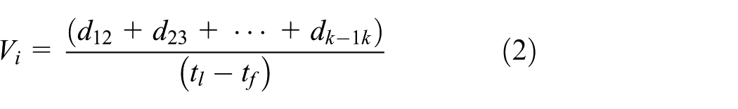
where
We denoted all sections in road network as
We queried an average speed of all road sections in the alternative trajectory
Calculation process
We were able to choose the best trajectory from the alternative plans based on the close degree between the evaluation objects and idealized goal, as shown in formula (3)

where
Here, we introduce the specific calculation steps, where the four attributes correspond to
Attribute normalization:
44
For speed matching degree, use
Weighted calculation,
Positive and negative solution calculations:
Object sort:
Optimal trajectory:
Empirical validation of the model
In this section, we used the actual data to validate the proposed trajectory reconstruction model.
Initial road network
From the distribution of equipment without consideration of rural roads, we chose an initial network of Ruian as a research area, which could reflect the city’s traffic characteristics and consisting of 35 nodes and 108 road sections (Figure 6) and Table 2 shows the road length.

Initial road network.
Partial information of road length.

Data preparation
We extracted 1 week’s records from the preprocessed data in section 1 and finally found more than 2000 complete trajectories information combined with the research network. Figure 7(a)–(c) shows three complete routes from three vehicle trajectory record sets.
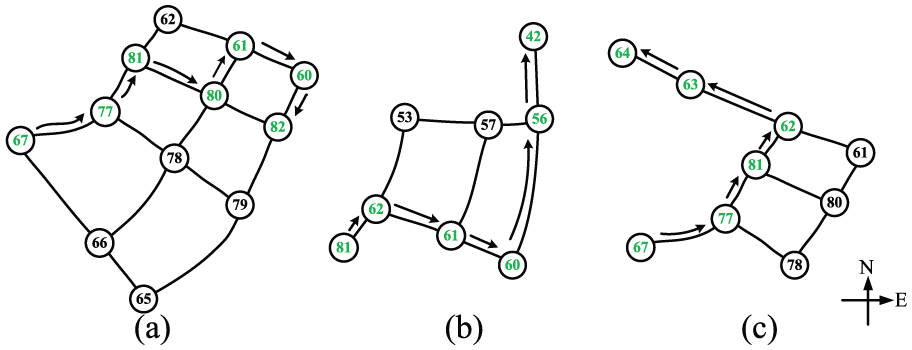
Three vehicles’ trajectories: Green circles and black arrows in (a), (b), (c) are three vehicles' trajectories respectively.
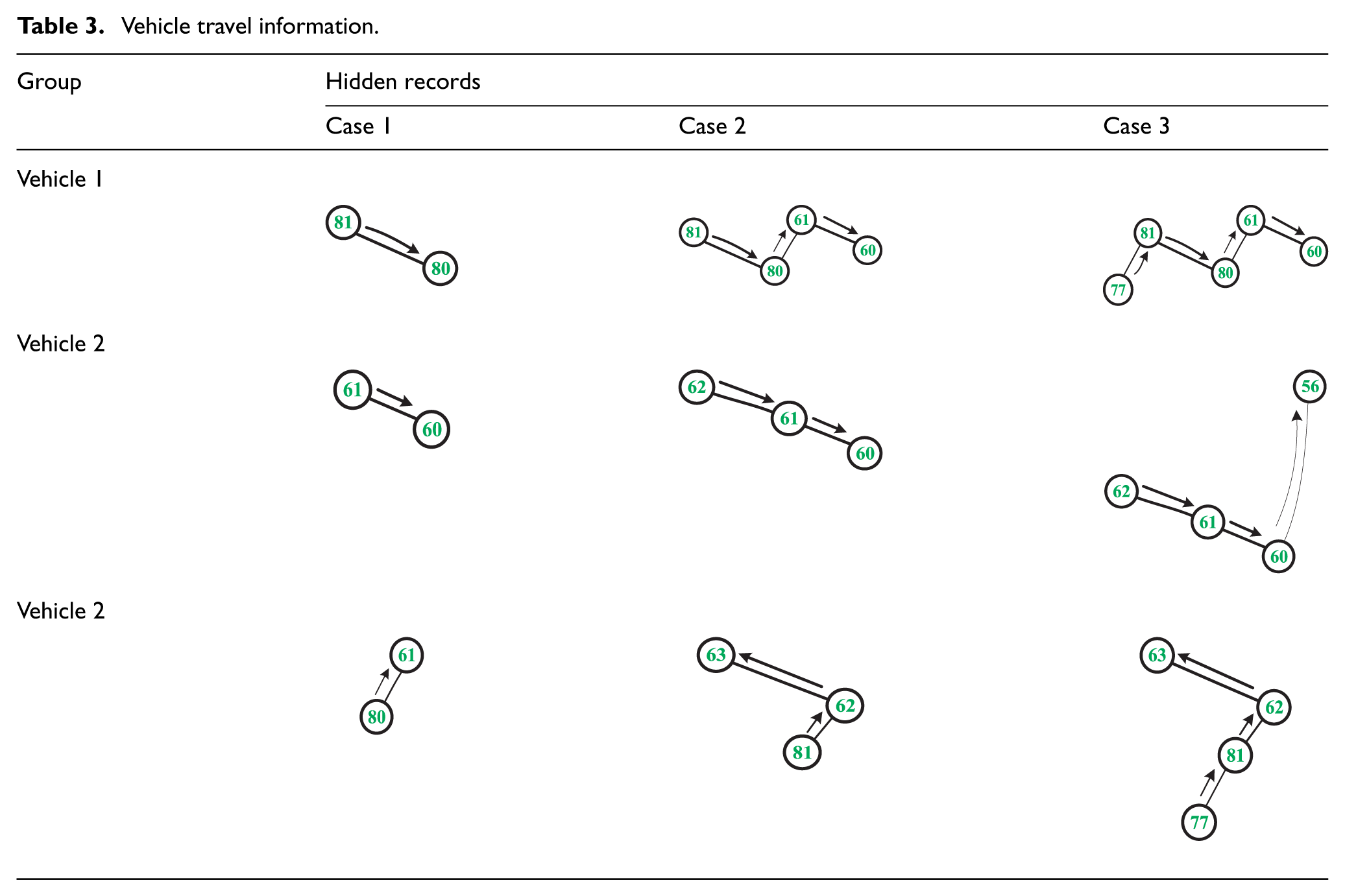
To provide a contrast between our experimental results and a real situation, we need some incomplete trajectories. This article supposed the missing vehicle trajectory records are irregular; then, we set three sets of experiments based on the missing number of trajectory points. We erased part of the vehicle trajectories and reconstructed them with the model. According to the time of trajectory records, we sorted and numbered them from 1 to the last one and then we generated random numbers from the serial number and deleted the corresponding records:
Missing 30% information. In the first case, we assumed that the vehicle trajectory points are lost about; for each complete trajectory, we randomly dropped 30% of them, as shown in Table 3, case 1, and two records were dropped out.
Missing 60% information. In the second case, we thought that the vehicle lost about 60% information and then randomly erased trajectory points (Table 3, case 2).
Missing 80% information. In the third case, the vehicle lost most trajectory information, and we removed all records in addition to the start and end points (Table 3, case 3).
Vehicle travel information.
With our method, we needed to obtain the actual speed and theoretical speed of each trajectory based on section 2. From the data and road network information, we calculated the average velocity per day of each section in the road network, as shown in Figure 8.

Road average speed throughout a week.
Experimental results
Single-trajectory experiment
With our method, we needed to obtain the actual speed and theoretical speed of each trajectory based on section 2. We mainly described the calculation process of vehicle 1 (Figure 7(a) and case 1), and we received three possible trajectories of vehicle 1: T1 = {67, 77, 81, 80, 61, 60, 82}, T2 = {67, 77, 78, 80, 61, 60, 82}, T3 = {67, 77, 81, 62, 61, 60, 82}, and we obtained each section’s velocity profile every 30 min in the road network throughout the day. This vehicle first appeared at 12:16:20, so we obtained the road sections’ average speed of each alternative trajectory during the time period 12:00:00–12:30:00, corresponding to the 23 time intervals (the blue dotted line in Figure 9). We found that the actual speeds on the three routes were 26.9, 25.1, and 23. The theoretical speeds were 26.9, 28.3, and 26.8.

The section speeds throughout the day in the road network.
Then, the initial decision matrix X was found:
In this article, we defined the weight vector
These results indicate that the first alternative trajectory was chosen as the “best” one, and in fact, it is the vehicle’s true trajectory.
Large-scale trajectory experiments
For the three groups of experiments from 2000 trajectories, we calculated the accuracy separately. These results indicate that the first case has better efficacy with 85%, the value of second case is 64%, and the third case has the lowest value about 43%. With the missing information increase, the accuracy of trajectory reconstruction tends to reduce, and we found that the more the information was lost, the more alternative trajectories were generated in the reconstruction model. This means the vehicle has many possible routes, which would improve the likelihood of the nonreal trajectories and reduce the accuracy of the result.
As shown in Figure 10, there is no significant difference in the accuracy of workdays (days 1–5) and weekend (days 6 and 7). In order to analyze the accuracy of the model throughout peak time and off-peak time, we calculated the traffic flow every 5 min in day 1 (Figure 11); correspondingly, we can obtain the accuracy of model within each hour of this day (Figure 12), and from the result, we found that there is no special difference between different hours.

The accuracy of three experiments throughout 7 days.

The traffic flow every 5 min in day 1.

The accuracy of the model within each hour in day 1.
For easy visual perception, we chose 10 trajectories from actual dataset and 3 experiments (Figure 13); case 1 is more similar to the actual. Furthermore, we have done more experiments to find the maximum missing rate 50%, and with this rate, we received an acceptable accuracy approximately 80%.

The trajectories from three experiment results and actual dataset.
In this section, we explained a common method for obtaining the vehicles’ travel portfolios based on the ALPR data, and this method also applies to other data (such as GPS information).
Concluding remarks
Properly mining vehicle travel information from ALPR data improves the understanding of the characteristics of commuting vehicles and the traffic state of the roadway network. This study proposed a general method to obtain a vehicle’s complete travel information. Based on the vehicle identification data, we organized these records according to the vehicle plate number and recognized a single trajectory from the vehicle’s records based on the travel time threshold B. We proposed a model to reconstruct incomplete vehicle trajectories through depth-first traversal and TOPSIS algorithm, and through known records, we found possible routes and set four attributes to evaluate the best trajectory, which included the speed parameter highly depending on the ALPR data. A numerical experiment using identification data from Ruian, China, was conducted to validate the effectiveness of the proposed model, where we did three groups of contrast experiments according to the missing degree of trajectory records; the results demonstrated that with the increase in missing records, the accuracy of the model would fall, and we also found that the results of model would not be affected by date and time of day. Based on the trajectory reconstruction model, we could obtain complete vehicle records, which provide a very reliable data support. Therefore, our findings are important for mining ALPR data and the analysis of vehicle commuting characteristics; it can also provide the basis for road condition evaluation and planning.
Although the proposed methods are promising for constructing a vehicle’s trajectories, some improvement is necessary. For instance, the model of the trajectory construction should be procedural and applied to the complex roadway network. In addition, there should be more research on travel patterns for all vehicles, such as the commuting distance analysis, which may help with the analysis of the traffic state of the road network.
Footnotes
Handling Editor: Liping Jiang
Declaration of conflicting interests
The author(s) declared no potential conflicts of interest with respect to the research, authorship, and/or publication of this article.
Funding
The author(s) disclosed receipt of the following financial support for the research, authorship, and/or publication of this article: This article is supported by the National Natural Science Foundation of China (51308021, U1564212, and 61773036), Beijing Natural Science Foundation (9172011), and Young Elite Scientist Sponsorship Program of the China Association for Science and Technology (2016QNRC001).