A scalable algorithm for the decomposition of minimally rigid graph

Abstract

The rigid graph needs to be decomposed to solve the multi-equilibrium problem of the multi-agent formation control based on navigation function method. In this paper, a theorem and a scalable algorithm based on the Henneberg sequence of graphs are proposed for the decomposition of minimally rigid graph. The theorem demonstrates that if graph G(V, E) is a minimally rigid graph, then it can be decomposed as G = G_t $\cup$ G_c, where G _t is a spanning tree of G and G _c contains the remaining edges and their vertices. Moreover, the scalable algorithm is given to construct G _t = (V _t , E _t ) and G _c = (V _c , E _c ), and assign the edges in E _c to n -- 2 distinct vertices in a scalable way via communication. Furthermore, a lemma is given to show when the number of vertices is less than eight, any edge can be chosen as the initialized edge, and the scalable algorithm mentioned above is always feasible. Finally, the effectiveness of the scalable algorithm is verified by numerical simulation.

Introduction

In recent years, multi-agent formation control has attracted the attention of multidisciplinary researchers due to its great advantages in specific applications, such as exploration, rescue, and surveillance. Formation control is a control technique in which many robots maintain a certain formation shape and adapt to environmental constraints while arriving at a destination. A formation system can be described from three main aspects: ¹ the geometrical shape, the communication topology, and the control strategy. There have been three approaches describing multi-agent formation, that is, displacement-based formation control,^2–6 distance-based formation control,^7–9 and bearing-only formation control.^10–13 Among the three approaches, distance-based formation control is regarded as a more ideal distributed approach, since the collision between the neighboring agents can be avoided. In the distance-based formation control, graph rigidity was crucial for the formation control, since it could maintain the specified geometry, as discussed in the work by Eren et al. ¹⁴ It is showed that if the communicated topology graph is rigid, the formation shape could be maintained. Therefore, how to achieve a globally stable rigid formation is crucial, and it has been extensively studied by many researchers.

The existing control law, such as the one proposed in the works by Eren et al. ¹⁴ and Krick et al., ¹⁵ only has local validity for small perturbations around the desired formation, and the multiple equilibria problem still existed. Dimarogonas and Johansson ⁹ show that the global stability to the desired formation can be achieved with negative gradient control law. However, the desired formation is assumed to be a tree, which is restrictive. So far, the multi-equilibrium problem for rigid formation with $n,n>3$ agents has not been well addressed. Inspired by the works by Dimarogonas and Johansson ⁹ and Krick et al., ¹⁵ the paper by Wang et al. ¹⁶ proposes an adaptive perturbation method for three agents, demonstrating that three agents could achieve the globally stable formation. This result is then extended to multi-agent system with $n$ agents, ¹⁷ and Trinh et al. ¹⁸ propose that in the absence of undesired stable equilibrium points and limit cycles, the multi-agent system could achieve the desired formation shape using the perturbed gradient method. Since the globally stable rigid formation can be achieved if and only if the communicating topology graph is a tree. Inspired by this, the minimally rigid graph can be decomposed as $G=G_t\cup G_c$ , where $G_t$ is a spanning tree of graph $G$ and $G_c$ contains the remaining edges and their vertices. It is expected that we can design a control strategy to drive the agents to the desired distance set in $G_c$ , and then, distances of remaining edges in $G_t$ will converge to the desired values using the standard gradient control strategy. Actually, the $n-2$ edges of $G_c$ can be assigned to $n-2$ distinct agents which will be controlled by the novel gradient method, and the remaining two agents will be driven by the standard negative gradient control law. The $n-2$ distinct agents, say agent $i$ , chooses any neighbor $l$ to determine the desired distance between the two agents. Therefore, it is crucial to know how to arrange $n-2$ agents to $n-2$ edges and how to choose the neighbor $l$ of the agent $i$ by which the desired distance is determined. Moreover, it is important to give an algorithm to show how to construct $G_t=(V_t,E_t)$ and $G_c=(V_c,E_c)$ and how to assign the edges in $E_c$ to $n-2$ distinct vertices in a scalable way via communication. This paper aims to solve these questions, thus the fully distributed control strategy for globally stable rigid formation can be obtained.

In this paper, a theorem based on the Henneberg sequence of graphs shows that the decomposition as $G=G_t\cup G_c$ is feasible, and then, $n-2$ edges in $G_c$ can be assigned to $n-2$ distinct vertices to determine the desired distance between the two neighboring agents. Furthermore, a scalable algorithm is given to show that $G_t=(V_t,E_t)$ and $G_c=(V_c,E_c)$ can be constructed in a local sense; at the same time, the edges in $E_c$ can be assigned to $n-2$ distinct vertices in a scalable way via communication. Finally, a lemma is given to show when the number of vertices is less than eight, any edge can be chosen as the initialized edge, and the scalable algorithm mentioned above is always feasible.

Preliminaries

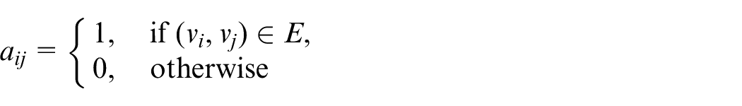
The information architecture of the formation system with $n$ agents can be modeled as a graph $G=\{V,E\}$ . $V(G)=\{v_1,v_2,\dots ,v_n\}$ denotes the vertex set, which represents agent $1,2,\dots ,n$ . And we model the edge set $E(G)\subset V(G)\times V(G)$ as the information structure. The edge $(v_i,v_j)\in E(G)$ denotes that agent $i$ can obtain information from agent $j$ . That is, the agent $j$ is a neighbor of agent $i$ , and $N_i$ denotes the set of all neighbors of agent $i$ . According to the graph $G=\{V,E\}$ , the weighted adjacency matrix $A\in \{0,1{\}}^{n\times n}$ can be defined as

$$a_{\mathrm{ij}}=\{\begin{array}{cc}1,\hfill & \mathrm{if}(v_i,v_j)\in E,\hfill \\ \multicolumn{1}{c}{0,}& \mathrm{otherwise}\hfill \end{array}$$

If $a_{\mathrm{ij}}=a_{\mathrm{ji}}$ for all $i,j\in \{1,\dots ,n\}$ , the weighted graph $G$ is undirected. Each edge $e_{\mathrm{ij}}\in E$ in graph $G$ is assigned to a constant $d_{\mathrm{ij}}=d_{\mathrm{ji}}$ , which means the desired distance that agents $i,j$ should preserve. Let $D=\{d_{\mathrm{ij}}:i\in V,j\in N_i\}$ . Then, a desired formation is represented as the framework $\{G,D\}$ . If all distance constraints specified by $D$ are satisfied and all distances between any pair of vertices in $G$ remain unchanged during the continuous displacement, then the formation $\{G,D\}$ is said to be rigid. Note that the rigid formation $\{G,D\}$ defined here is equivalent to the rigid graph $G$ defined in the work by Asimow and Roth. ¹⁹ A graph $G$ is said to be minimally rigid if it is rigid and has no graphs with the same vertices but fewer edges. ²⁰ In this paper, if the information architecture graph $G$ is minimally rigid, the formation $\{G,D\}$ is minimally rigid. The following lemma gives the numerical relationship between the number of nodes and the number of edges in the minimally rigid graph.

Lemma 1

A graph $G(V,E)$ with $|V|>1$ is minimally rigid if and only if $|E|=2|V|-3$ , and for all $E\prime \subseteq E,E\prime \ne z\varnothing$ , there holds $|E\prime |\le 2|V(E\prime )|-3$ , where $V(E\prime )$ is the set of vertices incident to $E\prime$ . ²¹

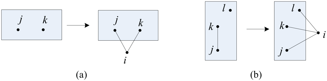
The construction of minimally rigid graphs usually consists of two graph operations: vertex addition operation and edge splitting operation. Let $j\mathrm{and}k$ be two different vertices of a minimally rigid graph $G(V,E)$ . A vertex addition operation involves adding a vertex $i$ and connecting it to $j$ and $k$ , as shown in Figure 1(a). Let $j,k$ , and $l$ be the three vertices of a minimally rigid graph, and there is an edge between $j$ and $k$ . An edge splitting operation includes deleting this edge, adding a vertex $i$ , and connecting it to $j,k$ , and $l$ , as shown in Figure 1(b). A sequence of graphs $G_2,G_3,\dots ,G_{|V|}$ is called a Henneberg sequence, which satisfies the following conditions: the graph $G_2$ is the complete graph with two vertices, and each graph $G_i(i\ge 3)$ can be obtained from $G_{i-1}$ by either a vertex addition operation or an edge splitting operation. ²²

Figure 1.

Representation of (a) vertex addition operation and (b) the edge splitting operation.

The following result gives a constructive method to form a minimally rigid graph.

Lemma 2

Every minimally rigid graph on more than one vertex can be obtained as the result of a Henneberg sequence. Moreover, all the graphs of such a sequence are minimally rigid. ²²

Scalable algorithm for the decomposition of graph $G$

Since the global stability of the multi-agent rigid formation can be achieved if and only if the topology is a tree, we need to decompose the rigid formation $G$ as $G=G_t\cup G_c$ , where $G_t$ is a spanning tree of $G$ and $G_c$ contains the remaining edges and their vertices. Then, the globally stable rigid formation can be achieved by designing an appropriate control algorithm. It is expected that we can design a control strategy to drive the agents to the desired distance set in $G_c$ , and then, distances of remaining edges in $G_t$ will converge to the desired values using the standard gradient control strategy. Supposing that the minimally rigid graph has $n$ vertices, then there are $n-1$ edges in $G_t$ . And by Lemma 1, there are $n-2$ edges in $G_c$ . That is, $n-2$ distinct agents should be arranged to look after the distances of $n-2$ edges, and then, the $n-2$ edges can achieve the desired distances using the novel control algorithm.

Now, we explain how to arrange $n-2$ agents to n-2 distinct edges and how to choose the neighbor $l$ of the agent $i$ by which the desired distance is determined. The next theorem shows that the minimally rigid graph can always accomplish such an assignment.

Theorem 1

Suppose the graph $G(V,E)$ is minimally rigid graph. There exists a decomposition $G=G_t\cup G_c$ , such that $n-2$ edges in $G_c$ can be assigned to $n-2$ distinct vertices.

Proof

We can prove Theorem 1 by induction. For $|V|=2$ , $E(G_c)$ is empty, and there is no edge to be assigned. For $|V|=3$ , $G_c$ contains only one edge, and the theorem is obviously true. Let us suppose the theorem is true for $|V|=n-1$ , that is, for any minimally rigid graph $G_{n-1}(V,E)$ with $|V|=n-1$ , there exists a decomposition $G_{n-1}=G_{t(n-1)}\cup G_{c(n-1)}$ such that $n-3$ edges in subgraph $G_c(n-1)$ can be assigned to $n-3$ distinct vertices of $G_{n-1}$ . Now, let us consider the case $|V|=n$ . By Lemma 2, any minimally rigid graph $G_n(V,E)$ with $|V|=n$ can be obtained from a minimally rigid graph $G_{n-1}(V,E)$ with $|V|=n-1$ by performing either a vertex addition operation or an edge splitting operation. We discuss two cases as follows.

• Case 1. The graph $G_n$ is obtained by performing a vertex addition on $G_{n-1}$ .

Let $j\mathrm{and}k$ be two distinct vertices of a minimally rigid graph $G_{n-1}$ . Let $G_{t(n-1)}$ be the spanning tree of $G_{n-1}$ supporting the induction hypothesis. Then, we can obtain a spanning tree $G_{t(n)}$ of graph $G_n$ from $G_{t(n-1)}$ by adding only one newly added edge, say $e_{\mathrm{ij}}$ . Thus, we have $G_{c(n)}=G_{c(n-1)}+e_{\mathrm{ik}}$ . Since all the edges in $G_{c(n-1)}$ have been assigned to $n-3$ distinct vertices of $G_{n-1}$ , we just need to assign the edge $e_{\mathrm{ik}}$ to the new vertex $i$ . The theorem is true in this case.

• Case 2. The graph $G_n$ is obtained by performing an undirected edge splitting on $G_{n-1}$ .

Suppose that $j,k,\mathrm{and}l$ are three distinct vertices of a minimally rigid graph $G_{n-1}$ and $e_{\mathrm{jk}}$ is an edge of $G_{n-1}$ . An edge splitting operation is shown in Figure 1(b). There are two possibilities shown in the following:

1. The edge $e_{\mathrm{jk}}$ is not in $G_{t(n-1)}$ supporting the induction hypothesis. From the induction hypothesis, we know that the edge $e_{\mathrm{jk}}$ had been assigned to either vertex $j$ or vertex $k$ . Without the loss of generality, suppose it is vertex $j$ . Since the edge $e_{\mathrm{jk}}$ is now removed, then vertex $j$ is unoccupied. Let $G_{t(n-1)}$ be the spanning tree of $G_{n-1}$ supporting the induction hypothesis. We can obtain a spanning tree $G_{t(n)}$ of graph $G_n$ from $G_{t(n-1)}$ by adding the edge $e_{\mathrm{ik}}$ . Now, we have $G_{c(n)}=G_{c(n-1)}+e_{\mathrm{ij}}+e_{\mathrm{il}}-e_{\mathrm{jk}}$ . Let $e_{\mathrm{ij}}$ be assigned to agent $j$ and $e_{\mathrm{il}}$ be assigned to agent $i$ . Then, the theorem is true in this subcase.

2. The edge $e_{\mathrm{jk}}$ is in $G_{t(n-1)}$ supporting the induction hypothesis. Since the edge $e_{\mathrm{jk}}$ is removed, we can obtain a spanning tree $G_{t(n)}$ of graph $G_n$ from $G_{t(n-1)}$ as $G_{t(n)}=G_{t(n-1)}-e_{\mathrm{jk}}+e_{\mathrm{ij}}+e_{\mathrm{ik}}$ . So, we have $G_{c(n)}=G_{c(n-1)}+e_{\mathrm{il}}$ . Let $e_{\mathrm{il}}$ be assigned to agent $i$ . Then, the theorem is true in this subcase.

Summarizing all the above possible cases, we conclude that the theorem is true. □

Next, we give an algorithm to show how to construct $G_t=(V_t,E_t)$ and $G_c=(V_c,E_c)$ and how to assign the edges in $E_c$ in a scalable way via communication.

Algorithm 1

% $V_s$ —the set of agents, to each of which an edge in $E_c$ has been assigned.

% $N_v^t$ —the set of agents which are both in $N_v$ and current $V_t$ .

% $|N_v^t|$ —the number of the agents in the set $N_v^t$ .

Step (i) [via communication between neighboring agents $v_1$ and $v_2$ ] Initiation.

(1) Let $V_0:=\{1,2,\dots ,n\}$ .

(2) Take a pair of neighboring agents $v_1,v_2\in V_0$ , and let $(V_t,E_t):=(v_1,v_2,(v_1,v_2))$ , $(V_c,E_c):=(\varnothing ,\varnothing )$ , $V_s:=\varnothing$ , and $n_{\mathrm{vt}}:=1$ .

Step (ii) [via communication between agent $v_i\in V_t$ and its neighbors] For the case when $v_i\in V_t$ can find a neighbor $v_k$ that does not belong to current $V_t$ , go to the next step; otherwise, go to the end.

Step (iii) If one of the following cases is satisfied, go to the next step; otherwise, let $V_0:=V_0\backslash \{v_1,v_2\}$ , go to Step (i)-(2).

$$\left(1\right)n_{\mathrm{vt}}=0,\mathrm{and}2\le |N_{v_k}^t|\le 3$$

(1)

$$\left(2\right)n_{\mathrm{vt}}\ne 0,\mathrm{and}1\le |N_{v_k}^t|\le 2$$

(2)

Step (iv) [via communication between neighboring agents $v_i$ and $v_k$ ] According to the values of $n_{\mathrm{vt}}$ and $|N_{v_k}^t|$ , do one of the following actions:

(1) For $n_{\mathrm{vt}}=0$ and $|N_{v_k}^t|=2$ , suppose $N_{v_k}^t=\{v_i,w\}$ . Let $V_t:=V_t+v_k$ , $E_t:=E_t+(v_i,v_k)$ , $V_c:=V_c+w$ , and $E_c:=E_c+(v_k,w)$ . Assign $(v_k,w)$ to $v_k$ , let $V_s:=V_s+v_k$ , and finally, let $n_{\mathrm{vt}}:=0$ , go to Step (ii).

(2) For $n_{\mathrm{vt}}=0$ and $|N_{v_k}^t|=3$ , suppose $N_{v_k}^t=\{v_i,w_1,w_2\}$ . Let $V_t:=V_t+v_k$ , $E_t:=E_t+(v_i,v_k)$ , $V_c:=V_c\cup \{w_1,w_2\}$ , and $E_c:=E_c\cup \{(v_k,w_1),(v_k,w_2)\}$ . Assign $(v_k,w_1)$ to $w_1$ , $(v_k,w_2)$ to $v_k$ , and let $V_s:=V_s\cup \{w_1,v_k\}$ , if $w_1\notin V_s$ ; otherwise, assign $(v_k,w_2)$ to $w_2$ , $(v_k,w_1)$ to $v_k$ , and let $V_s:=V_s\cup \{w_2,v_k\}$ . Finally, let $n_{\mathrm{vt}}:=1$ , go to Step (ii).

 (% The proof of Theorem 1 ensures that at least one of $w_1,w_2$ does not belong to $V_s$ .)

(3) For $n_{\mathrm{vt}}\ne 0$ and $|N_{v_k}^t|=1$ , $N_{v_k}^t$ must be $\{v_i\}$ . In this case, let $V_t:=V_t+v_k$ , $E_t:=E_t+(v_i,v_k)$ , and finally, let $n_{\mathrm{vt}}:=0$ , go to Step (ii).

(4) For $n_{\mathrm{vt}}\ne 0$ and $|N_{v_k}^t|=2$ , suppose $N_{v_k}^t=\{v_i,w\}$ . Let $V_t:=V_t+v_k$ , $E_t:=E_t+(v_i,v_k)$ , $V_c:=V_c+w$ , $E_c:=E_c+(v_k,w)$ , assign $(v_k,w)$ to $v_k$ , let $V_s:=V_s+v_k$ , and finally, let $n_{\mathrm{vt}}:=1$ , go to Step (ii).

Step (v). End, return $(V_t,E_t,V_c,E_c,V_s)$ .

Remark 1

Theorem 1 can guarantee the feasibility of Algorithm 1, and the output of Algorithm 1 is always there, and then, we can always find the appropriate initialized edge to make the algorithm work.

Remark 2

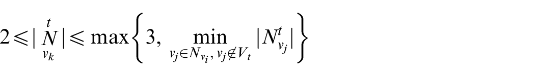
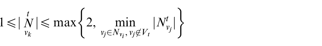
Algorithm 1 works for redundantly rigid graphs, and the global rigid graphs belong to redundantly rigid graphs, so it is also suitable for the global rigid ones. For the redundantly rigid graph, Algorithm 1 can be modified as follows. In this case, equations (1) and (2) should be replaced by

$$2\le \left|\underset{v_k}{\overset{t}{N}}\right|\le \max \left\{3,\underset{v_j\in N_{v_i},v_j\notin V_t}{\min }\left|N_{v_j}^t\right|\right\}$$

and

$$1\le \left|\underset{v_k}{\overset{t}{N}}\right|\le \max \left\{2,\underset{v_j\in N_{v_i},v_j\notin V_t}{\min }\left|N_{v_j}^t\right|\right\}$$

respectively; and in Step (iv), agent $v_k$ should ignore redundant neighbors in $N_{v_k}^t$ . In such a way, $G_t\cup G_c$ generated by the algorithm is a minimally rigid graph, which is just a subgraph of the redundantly rigid graph $G$ . Let the agents ignore the redundant neighbors, if the novel formation control algorithm can globally stabilize the minimally rigid formation, the redundantly rigid formation can also be globally stabilized.

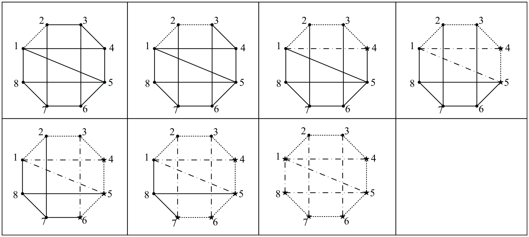
Note that the output of the algorithm is not necessarily unique. Figure 2 shows an execution of the algorithm. The algorithm initiates from the edge $(1,2)$ . In Figure 2, the dashed edges belong to $G_t$ , the dashed–dotted edges belong to $G_c$ , and the vertices marked by star denote the vertices in $V_s$ . Therefore, we can add control constrains to agent 4 for looking after $r_{41}$ , to agent 5 for looking after $r_{51}$ , to agent 6 for looking after $r_{63}$ , to agent 7 for looking after $r_{72}$ , to agent 8 for looking after $r_{85}$ , and to agent 1 for looking after $r_{81}$ , respectively.

Figure 2.

Execution of Algorithm 1.

In contrast to the previous example, when the initialized edge is chosen unprofitably, Algorithm 1 is not feasible, and we cannot obtain the decomposition of the graph $G$ , which will be shown in the simulation. However, if we choose the appropriate initialized edge which is always existed, Algorithm 1 is feasible. Next, we give a lemma to demonstrate that when the number of vertices is less than eight, then any edge can be chosen as the initialized edge, and the scalable algorithm mentioned above is always feasible.

Lemma 3

If the graph is minimally rigid, when the number of vertices is less than eight, the scalable Algorithm 1 mentioned above is always feasible.□

Proof

In Step (iii)-(2), $n_{\mathrm{vt}}=1$ , the algorithm is always feasible. At each step, when $n_{\mathrm{vt}}=1$ , the subgraph $G(V_t)$ is a minimally rigid graph.

When $n_{\mathrm{vt}}=0$ , the subgraph $G(V_t)$ is not minimally rigid. Suppose that Step (iii)-(1) is not feasible, we have $|N_{\mathrm{vk}}^t|=1$ .

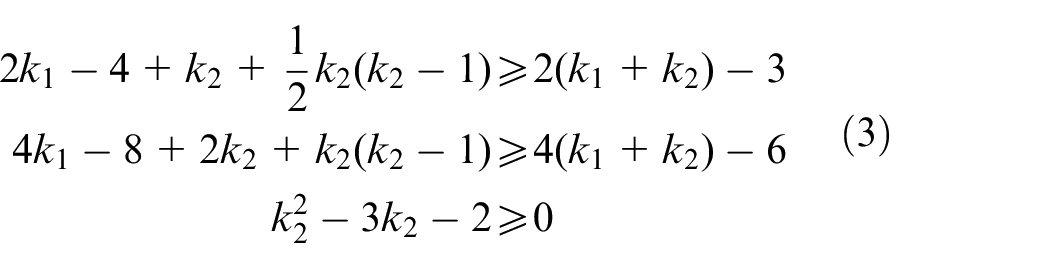
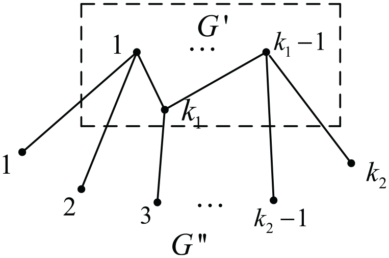
As shown in Figure 3, the subgraph $G\prime$ which is not minimally rigid has $k_1(k_1\ge 3)$ vertices, and graph $G"$ is the minimally rigid graph which has $k_1+k_2$ vertices. From the hypothesis, we know that there does not exist a vertex $v_k$ with $|N_{v_k}^t|$ being 2 or 3, then $|N_{\mathrm{vk}}^t|=1$ . Therefore, there are only $k_2$ edges between $k_2$ vertices and the subgraph $G\prime$ . Moreover, there are at most $(1/2)(k_2(k_2-1))$ edges between $k_2$ vertices. Then, we have the following equation

$$\begin{array}{c}\multicolumn{1}{c}{2k_1-4+k_2+\frac{1}{2}{k}_2(k_2-1)\ge 2(k_1+k_2)-3}\\ \multicolumn{1}{c}{4k_1-8+2k_2+k_2(k_2-1)\ge 4(k_1+k_2)-6}\\ \multicolumn{1}{c}{k_2^2-3k_2-2\ge 0}\end{array}$$

(3)

The left of the equation means the most edges of the current graph. From equation (3), we have $k_2\ge (3+\sqrt{17})/2$ , then we also have $k_1+k_2\ge 7.57$ , which means that when the number of vertices is more than seven, the graph $G"$ may be minimally rigid. Otherwise, the hypothesis does not hold. Therefore, we can conclude that when the number of vertices is less than eight, the scalable Algorithm 1 mentioned above is always feasible.□

Figure 3.

Minimally rigid graph $G"$ and $G\prime \subset G"$ .

Simulations

In this section, we do some numerical simulations to illustrate the effectiveness of the scalable algorithm. The simulation environment: Intel^® Core™ i5-4210U CPU at 1.70 GHz, 2.40 GHz, RAM 4.00 GB. And the simulation software is Matlab 2014b. Let $N$ denotes the number of agents of a minimally rigid graph $G=(V,E)$ and $T$ denotes the execution time taken to complete the simulation. If $N=20$ , then $T=0.1\mathrm{s}$ ; If $N=40$ , then $T=0.148\mathrm{s}$ ; If $N=100$ , then $T=0.281\mathrm{s}$ ; If $N=200$ , then $T=0.491\mathrm{s}$ . From the above data, we can conclude that for a given computational platform, the growth rate of the execution time is almost half of that of the agent number, and the execution time is short. Then, the proposed scalable Algorithm 1 can be applied in practice.

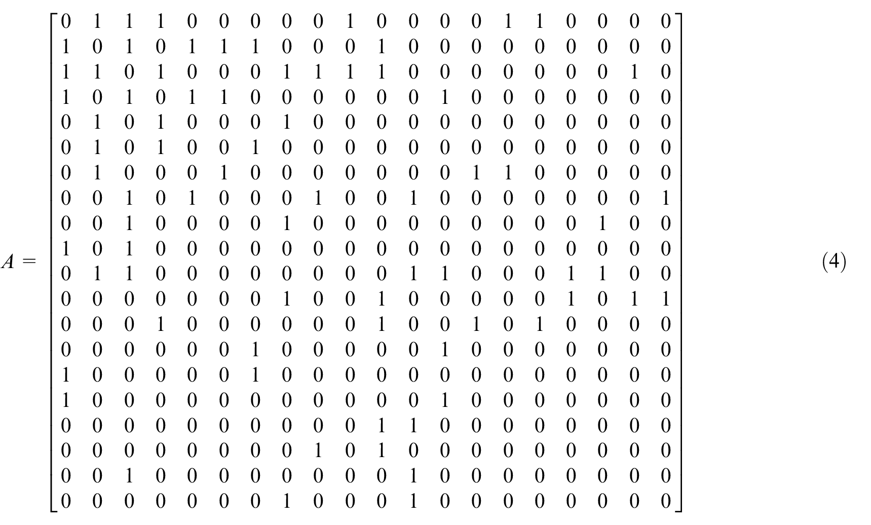
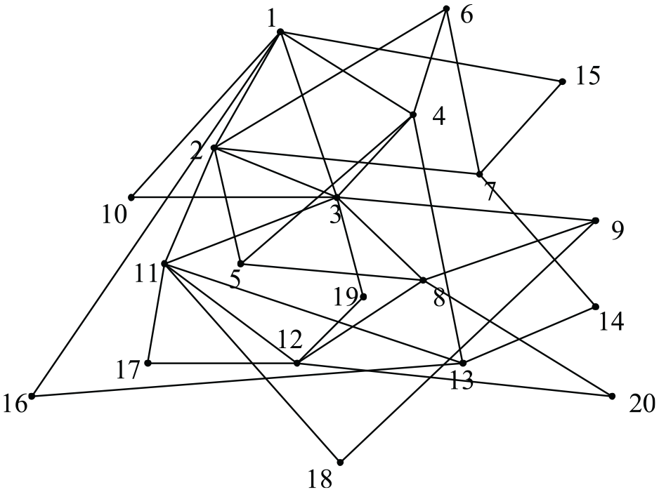
Here, we only give one of the simulations. First, a minimally rigid graph $G=(V,E),V=\{1,2,\dots ,20\}$ is constructed based on the Henneberg sequence of graphs. The graph $G$ is shown in Figure 4, and the corresponding adjacent matrix $A$ of graph $G$ is

$$A=\left[\begin{array}{cccccccccccccccccccc}0\hfill & 1\hfill & 1\hfill & 1\hfill & 0\hfill & 0\hfill & 0\hfill & 0\hfill & 0\hfill & 1\hfill & 0\hfill & 0\hfill & 0\hfill & 0\hfill & 1\hfill & 1\hfill & 0\hfill & 0\hfill & 0\hfill & 0\hfill \\ \multicolumn{1}{c}{1}& 0\hfill & 1\hfill & 0\hfill & 1\hfill & 1\hfill & 1\hfill & 0\hfill & 0\hfill & 0\hfill & 1\hfill & 0\hfill & 0\hfill & 0\hfill & 0\hfill & 0\hfill & 0\hfill & 0\hfill & 0\hfill & 0\hfill \\ \multicolumn{1}{c}{1}& 1\hfill & 0\hfill & 1\hfill & 0\hfill & 0\hfill & 0\hfill & 1\hfill & 1\hfill & 1\hfill & 1\hfill & 0\hfill & 0\hfill & 0\hfill & 0\hfill & 0\hfill & 0\hfill & 0\hfill & 1\hfill & 0\hfill \\ \multicolumn{1}{c}{1}& 0\hfill & 1\hfill & 0\hfill & 1\hfill & 1\hfill & 0\hfill & 0\hfill & 0\hfill & 0\hfill & 0\hfill & 0\hfill & 1\hfill & 0\hfill & 0\hfill & 0\hfill & 0\hfill & 0\hfill & 0\hfill & 0\hfill \\ \multicolumn{1}{c}{0}& 1\hfill & 0\hfill & 1\hfill & 0\hfill & 0\hfill & 0\hfill & 1\hfill & 0\hfill & 0\hfill & 0\hfill & 0\hfill & 0\hfill & 0\hfill & 0\hfill & 0\hfill & 0\hfill & 0\hfill & 0\hfill & 0\hfill \\ \multicolumn{1}{c}{0}& 1\hfill & 0\hfill & 1\hfill & 0\hfill & 0\hfill & 1\hfill & 0\hfill & 0\hfill & 0\hfill & 0\hfill & 0\hfill & 0\hfill & 0\hfill & 0\hfill & 0\hfill & 0\hfill & 0\hfill & 0\hfill & 0\hfill \\ \multicolumn{1}{c}{0}& 1\hfill & 0\hfill & 0\hfill & 0\hfill & 1\hfill & 0\hfill & 0\hfill & 0\hfill & 0\hfill & 0\hfill & 0\hfill & 0\hfill & 1\hfill & 1\hfill & 0\hfill & 0\hfill & 0\hfill & 0\hfill & 0\hfill \\ \multicolumn{1}{c}{0}& 0\hfill & 1\hfill & 0\hfill & 1\hfill & 0\hfill & 0\hfill & 0\hfill & 1\hfill & 0\hfill & 0\hfill & 1\hfill & 0\hfill & 0\hfill & 0\hfill & 0\hfill & 0\hfill & 0\hfill & 0\hfill & 1\hfill \\ \multicolumn{1}{c}{0}& 0\hfill & 1\hfill & 0\hfill & 0\hfill & 0\hfill & 0\hfill & 1\hfill & 0\hfill & 0\hfill & 0\hfill & 0\hfill & 0\hfill & 0\hfill & 0\hfill & 0\hfill & 0\hfill & 1\hfill & 0\hfill & 0\hfill \\ \multicolumn{1}{c}{1}& 0\hfill & 1\hfill & 0\hfill & 0\hfill & 0\hfill & 0\hfill & 0\hfill & 0\hfill & 0\hfill & 0\hfill & 0\hfill & 0\hfill & 0\hfill & 0\hfill & 0\hfill & 0\hfill & 0\hfill & 0\hfill & 0\hfill \\ \multicolumn{1}{c}{0}& 1\hfill & 1\hfill & 0\hfill & 0\hfill & 0\hfill & 0\hfill & 0\hfill & 0\hfill & 0\hfill & 0\hfill & 1\hfill & 1\hfill & 0\hfill & 0\hfill & 0\hfill & 1\hfill & 1\hfill & 0\hfill & 0\hfill \\ \multicolumn{1}{c}{0}& 0\hfill & 0\hfill & 0\hfill & 0\hfill & 0\hfill & 0\hfill & 1\hfill & 0\hfill & 0\hfill & 1\hfill & 0\hfill & 0\hfill & 0\hfill & 0\hfill & 0\hfill & 1\hfill & 0\hfill & 1\hfill & 1\hfill \\ \multicolumn{1}{c}{0}& 0\hfill & 0\hfill & 1\hfill & 0\hfill & 0\hfill & 0\hfill & 0\hfill & 0\hfill & 0\hfill & 1\hfill & 0\hfill & 0\hfill & 1\hfill & 0\hfill & 1\hfill & 0\hfill & 0\hfill & 0\hfill & 0\hfill \\ \multicolumn{1}{c}{0}& 0\hfill & 0\hfill & 0\hfill & 0\hfill & 0\hfill & 1\hfill & 0\hfill & 0\hfill & 0\hfill & 0\hfill & 0\hfill & 1\hfill & 0\hfill & 0\hfill & 0\hfill & 0\hfill & 0\hfill & 0\hfill & 0\hfill \\ \multicolumn{1}{c}{1}& 0\hfill & 0\hfill & 0\hfill & 0\hfill & 0\hfill & 1\hfill & 0\hfill & 0\hfill & 0\hfill & 0\hfill & 0\hfill & 0\hfill & 0\hfill & 0\hfill & 0\hfill & 0\hfill & 0\hfill & 0\hfill & 0\hfill \\ \multicolumn{1}{c}{1}& 0\hfill & 0\hfill & 0\hfill & 0\hfill & 0\hfill & 0\hfill & 0\hfill & 0\hfill & 0\hfill & 0\hfill & 0\hfill & 1\hfill & 0\hfill & 0\hfill & 0\hfill & 0\hfill & 0\hfill & 0\hfill & 0\hfill \\ \multicolumn{1}{c}{0}& 0\hfill & 0\hfill & 0\hfill & 0\hfill & 0\hfill & 0\hfill & 0\hfill & 0\hfill & 0\hfill & 1\hfill & 1\hfill & 0\hfill & 0\hfill & 0\hfill & 0\hfill & 0\hfill & 0\hfill & 0\hfill & 0\hfill \\ \multicolumn{1}{c}{0}& 0\hfill & 0\hfill & 0\hfill & 0\hfill & 0\hfill & 0\hfill & 0\hfill & 1\hfill & 0\hfill & 1\hfill & 0\hfill & 0\hfill & 0\hfill & 0\hfill & 0\hfill & 0\hfill & 0\hfill & 0\hfill & 0\hfill \\ \multicolumn{1}{c}{0}& 0\hfill & 1\hfill & 0\hfill & 0\hfill & 0\hfill & 0\hfill & 0\hfill & 0\hfill & 0\hfill & 0\hfill & 1\hfill & 0\hfill & 0\hfill & 0\hfill & 0\hfill & 0\hfill & 0\hfill & 0\hfill & 0\hfill \\ \multicolumn{1}{c}{0}& 0\hfill & 0\hfill & 0\hfill & 0\hfill & 0\hfill & 0\hfill & 1\hfill & 0\hfill & 0\hfill & 0\hfill & 1\hfill & 0\hfill & 0\hfill & 0\hfill & 0\hfill & 0\hfill & 0\hfill & 0\hfill & 0\hfill \end{array}\right]$$

(4)

Figure 4.

The rigid graph $G$ .

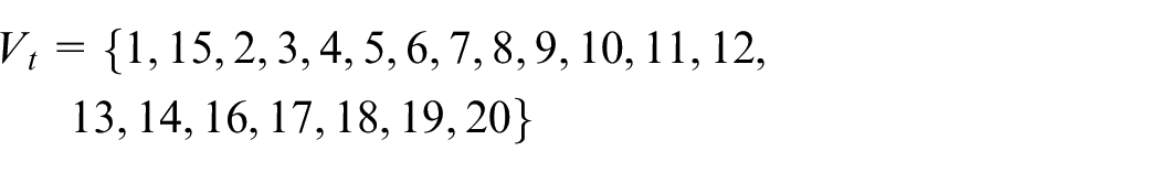
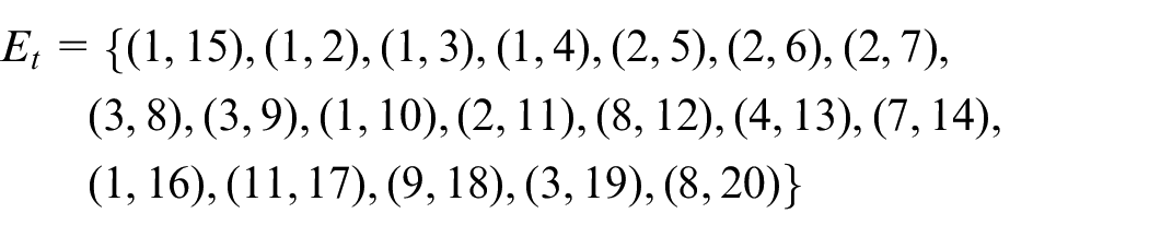
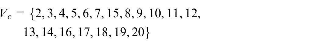
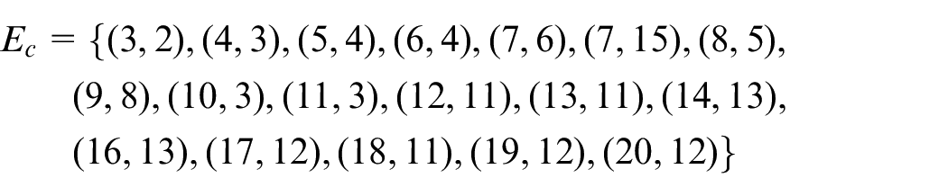
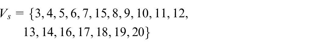
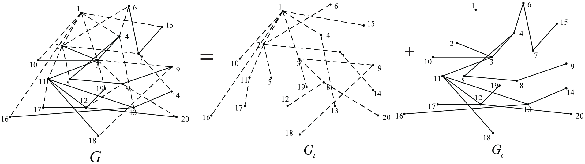
Second, based on Algorithm 1, if we choose the appropriate initialized edge, the minimally rigid graph $G$ can be decomposed as $G=G_t\cup G_c$ , where $G_t=(V_t,E_t)$ , $G_c=(V_c,E_c)$ , and the edges in $E_c$ are assigned to $n-2$ distinct vertices belong to $V_s$ in a scalable way via communication. We choose the initialized edge as (1,15; the initialized edge is not unique), and the output of the algorithm is as follows

$$\begin{array}{c}{V}_t=\{1,15,2,3,4,5,6,7,8,9,10,11,12,\hfill \\ 13,14,16,17,18,19,20\}\hfill \end{array}$$

$$\begin{array}{c}{E}_t=\{(1,15),(1,2),(1,3),(1,4),(2,5),(2,6),(2,7),\hfill \\ (3,8),(3,9),(1,10),(2,11),(8,12),(4,13),(7,14),\hfill \\ (1,16),(11,17),(9,18),(3,19),(8,20)\}\hfill \end{array}$$

$$\begin{array}{c}{V}_c=\{2,3,4,5,6,7,15,8,9,10,11,12,\hfill \\ 13,14,16,17,18,19,20\}\hfill \end{array}$$

$$\begin{array}{c}{E}_c=\{(3,2),(4,3),(5,4),(6,4),(7,6),(7,15),(8,5),\hfill \\ (9,8),(10,3),(11,3),(12,11),(13,11),(14,13),\hfill \\ (16,13),(17,12),(18,11),(19,12),(20,12)\}\hfill \end{array}$$

$$\begin{array}{c}{V}_s=\{3,4,5,6,7,15,8,9,10,11,12,\hfill \\ 13,14,16,17,18,19,20\}\hfill \end{array}$$

where $V_s$ denotes the set of agents, to each of which the corresponding edge in $E_c$ has been assigned. The decomposition of graph $G$ is shown in Figure 5. In Figure 5, the dashed edges belong to $G_t$ and the solid edges belong to $G_c$ . In contrast to the previous initialized edge, when the initialized edge is chosen as (12,20), Algorithm 1 is not feasible, and we cannot obtain the decomposition of the graph $G$ . However, if we choose the appropriate initialized edge which is always existed, Algorithm 1 is feasible.

Figure 5.

The decomposition of graph $G$ .

Conclusion

In this paper, a theorem based on the Henneberg sequence of graphs shows that if graph $G(V,E)$ is minimally rigid graph, the graph $G$ can be decomposed as $G=G_t\cup G_c$ and $n-2$ edges in $G_c$ can be assigned to $n-2$ distinct vertices. Furthermore, an algorithm is given to construct $G_t=(V_t,E_t)$ and $G_c=(V_c,E_c)$ and assign the edges in $E_c$ to $n-2$ distinct vertices in a scalable way via communication. Currently, it is demonstrated that when the number of vertices is less than eight, the scalable algorithm is always feasible. How to design a globally stable control algorithm for the rigid formation is still a challenging problem in the future.