
Abstract
Global positioning system is an important space information network for location service. However, the satellite signal is attenuated or even blocked in indoor environment. To make up for the defect of global positioning system, IEEE 802.11 wireless local area network (Wi-Fi) infrastructure is proposed to relay the task of positioning in indoor scenario with their superiority of being widely deployed. In Wi-Fi indoor localization application, received signal strength indicator is the most prevalent parameter. From the former literature, it was supposed to be Gaussian distribution. In this article, we first formulate the received signal in a multipath channel based on the IEEE 802.11 standard, then we derive the probability density function of received signal strength indicator and it is proved to be a noncentral Chi-square distribution. Finally, the correctness of the distribution is verified from the aspect of noncentral parameter in an experiment system.
Keywords
Introduction
Indoor location sensing systems have been extensively studied for the past two decades and continuously attracted vast research efforts with the huge growing of mobile computing. Although global positioning system (GPS) is the most widely used space information network for outdoor location sensing technology, there are several drawbacks which make GPS impossible to be used as an indoor positioning tool. Due to the non-line-of-sight (NLOS) transmission between the satellites and the receivers, and the special hardware requirement, the GPS has poor indoor coverage and insufficient accuracy. 1 With the fact that users spend about 89% of their time indoors, precise indoor localization is still a challenging problem and has been gaining growing interest from a wide range of applications, for example, location detection of assets in a warehouse, location detection of medical personnel or equipment in a hospital, and emergency personnel positioning in a disaster area. 2
Wireless local area network (WLAN) technique, which is based on IEEE 802.11 standard, namely, Wi-Fi, is operating in the 2.4 GHz industrial, scientific, and medical (ISM) band and has become very popular in public hotspots and enterprise locations during the last few years. 3 With a typical gross bit rate of 11, 54, or 108 Mbps and a range of 50–100 m, IEEE 802.11 is currently the dominant local wireless networking standard. Nowadays, Wi-Fi has been widely deployed in indoor public places, which makes Wi-Fi-based wireless indoor location applications become one of the most attractive research topics in recent years. Therefore, Wi-Fi is an important infrastructure to relay the task of positioning in indoor scenario without the assistance of GPS. Thus, Wi-Fi-based indoor location sensing system is considered in this article.
First, several representative Wi-Fi-based indoor location sensing systems are compared in Table 1, where the localization parameters can be mainly classified as received signal strength indicator (RSSI), channel state information (CSI), direction of arrival (DOA), round-trip time (RTT), and time of arrival (TOA). We show the properties of these parameters from four aspects, namely, scheme of mapping, system, localization algorithm, and precision. The scheme of mapping can be categorized into geometric mapping and fingerprinting mapping. The localization algorithms include k-nearest-neighbor (KNN), genetic algorithm, prior NLOS measurements correction (PNMC), and so on. The localization parameters, namely, RSSI, CSI, DOA, and TOA are calculated by the sampling values. On the meanwhile, RTT value is extracted from the field of the IEEE 802.11 frame. RSSI is the power of one frame, CSI is estimated by the pilots of the frame, DOA is calculated by the phase difference between the signals received by various antennas, and TOA is the transmission time between the transmitter and receiver.
Wi-Fi-based indoor location sensing systems.
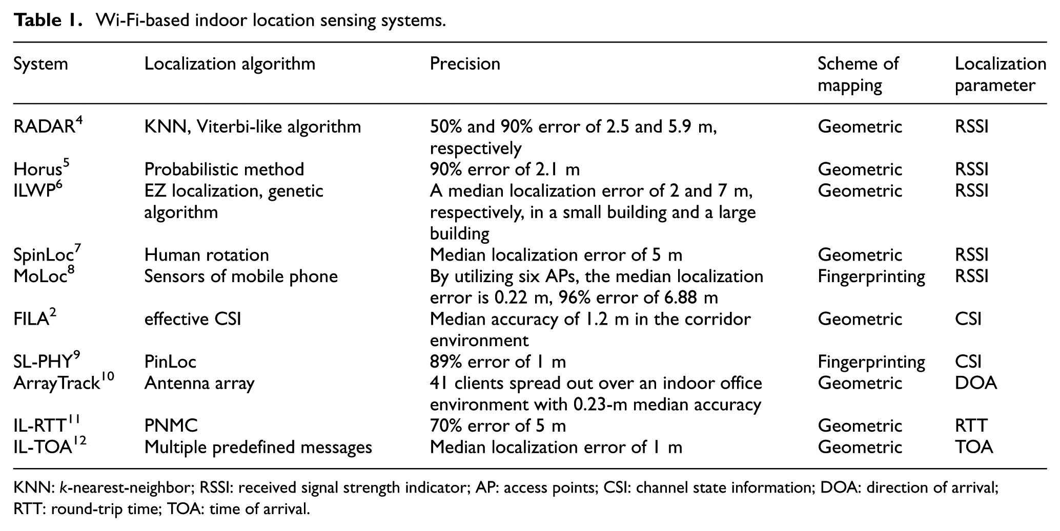
KNN: k-nearest-neighbor; RSSI: received signal strength indicator; AP: access points; CSI: channel state information; DOA: direction of arrival; RTT: round-trip time; TOA: time of arrival.
From Table 1, we can conclude that the RSSI is a prevalent parameter in indoor localization. Theoretically, RSSI decreases monotonically with distance in free space, so that the distance of the target can be calculated from RSSI.
13
Although RSSI can achieve meter-level localization accuracy in some environments, it suffers from dramatic performance degradation in a lot of complex situations. It is mentioned in Wu et al.
14
that RSSI is measured from the radio frequency (RF) signal at a per packet level, thus it is difficult to obtain an accurate value of decimeter. It is claimed in Wang et al.
15
that RSSI values are highly random and its correlation with propagation distance is loose due to shadowing fading and multipath effects. In the literature,3,5 the statistic of RSSI is modeled as Gaussian distribution. In this article, we derive the probability density function (PDF) of the RSSI based on the orthogonal frequency-division multiplexing (OFDM) signal of IEEE 802.11 standard in a general multipath scenario, which satisfies a noncentral Chi-square
We formulate the received 802.11 signal in multipath transmission environment.
We calculate the PDF of RSSI which satisfies noncentral
We implement a test system to verify the 802.11 signal RSSI. Experimental results demonstrate that the distribution for PDF of power is noncentral
The rest of this article is organized as follows. In section “Preliminaries,” we introduce the OFDM signal of IEEE 802.11 standard. The PDF of RSSI in a multipath scenario is derived in section “PDF of RSSI.” The experimental results are presented in section “Experimental results.” Finally, conclusions are given in section “Conclusion.”
Preliminaries
In this section, we first introduce the general OFDM signal and then the IEEE 802.11 OFDM training structure.
OFDM signal
OFDM is widely used in IEEE 802.11a/g/n and WiMAX, and it is the critical technique for future standards such as 3GPP LTE. It is a bandwidth-efficient digital multicarrier modulation scheme for wideband wireless communications, as shown in Figure 1. In OFDM, the overall spectrum band is divided into many small and partially overlapped signal-carrying frequency bands named subcarriers. For the transmitter, each carrier takes part of the data to be transmitted on an OFDM carrier signal. The data are first performed via an inverse fast Fourier transform (IFFT). The real and imaginary components are then converted to analog domain by digital-to-analog converters (DACs). Upon receiving the signals, the signal are sampled by analog-to-digital converters (ADCs) and passed to a demodulation process chain. A fast Fourier transform (FFT) convert the waveform to frequency domain, as illustrated in Figure 2. 16
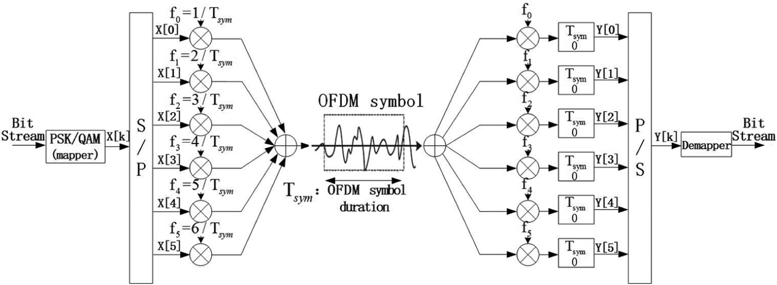
OFDM modulation/demodulation: N = 6 (six subcarriers).

Block diagram of transmitter and receiver in an OFDM system.
IEEE 802.11 OFDM
The physical layer convergence procedure (PLCP) preamble field is used for synchronization. 17 It consists of 10 short symbols and 2 long symbols which are shown in Figure 3. The timing stamps described here shown in Figure 3 are for 20 MHz channel spacing. They are doubled for half-clocked (i.e. 10 MHz) channel spacing and are quadrupled for quarter-clocked (i.e. 5 MHz) channel spacing. It is shown that t1–t10 denote short training symbols, T1 and T2 denote the long training symbols. The PLCP preamble is followed by the signal field and data. The total training length is 16 μs. The dashed boundaries in the figure denote repetitions due to the periodicity of the inverse Fourier transform.
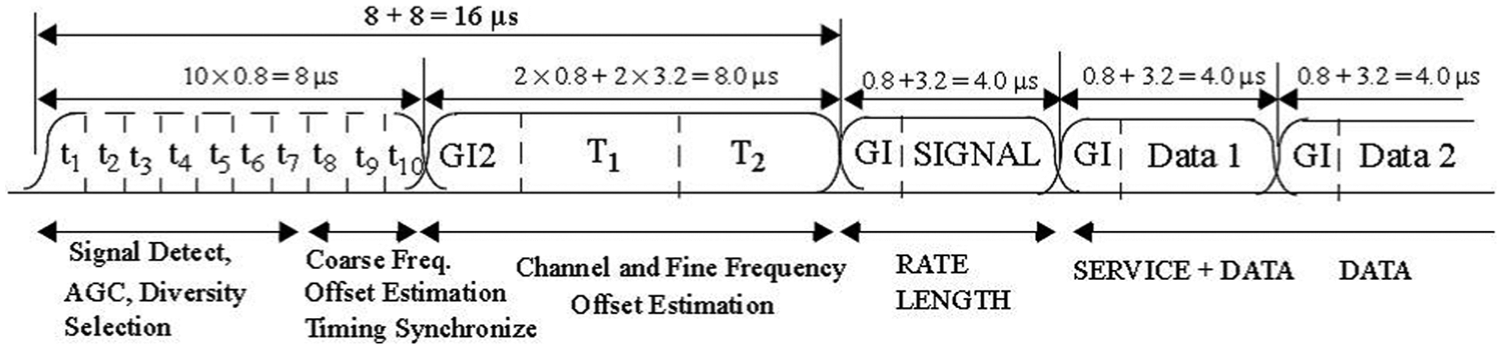
OFDM training structure.
PDF of RSSI
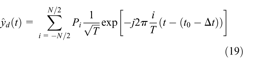
Assume N is the number of transmitted subcarriers, and

where

Assume an M-path multipath channel, which can be represented as

where

Substituting equations (2) and (3) into equation (4), we obtain

where

After the down converter and low-pass filter, the signal can be described as

where

as the equivalent channel fading coefficient of the kth path, then equation (7) can be represented as
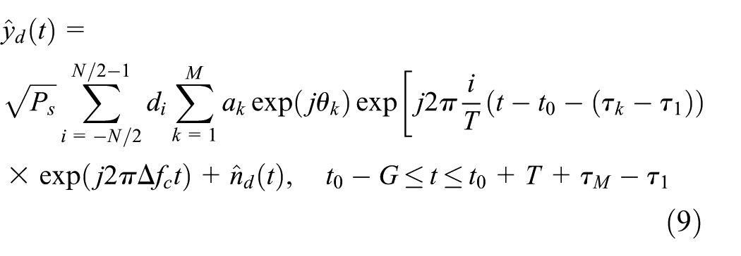
As

equation (9) can be shorten as

According to equation (11), the transmission of multipath signal is shown in Figure 4.
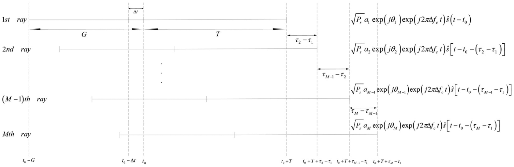
The transmission of multipath signal.
Now, we focus on the statistical analysis of the RSSI. In the implementation of receiver design, the frequency shift, namely,

Due to that OFDM signal is composed of orthogonal subcarriers, we have the N orthogonal waveforms as

The coordinate of the

It is easy to verify that


If

satisfies complex Gaussian distribution with18,19


Therefore, equation (14) can be reformulated as

Hence, equation (12) can be represented as
The RSSI can be calculated as

where
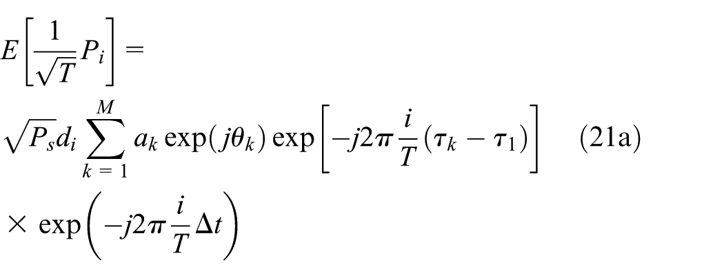
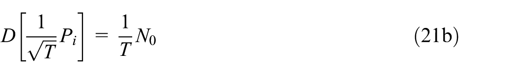
Thus,

Finally, the PDF of RSSI can be calculated as

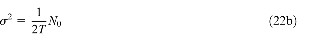
The mean value and variance of a noncentral Chi-square distribution can be written as, respectively


Thus, the noncentral parameter can be calculated as

Experimental results
In order to verify the statistical analysis of RSSI, we implement an experiment, where a signal analyzer, namely, Key Sight N9030A is utilized to receive the signals. As shown in Figure 5, a wireless router emits IEEE 802.11n signal, and the signal is transmitted over a multipath environment; at the receiver, it is sampled by the signal analyzer. The bandwidth of signal is 20 MHz, as shown by Figure 6, there are 14 channels, and the signal could be transmitted on one of them. We can see that the un-adjacent channels are 1, 6, and 11.

RSSI experiment.
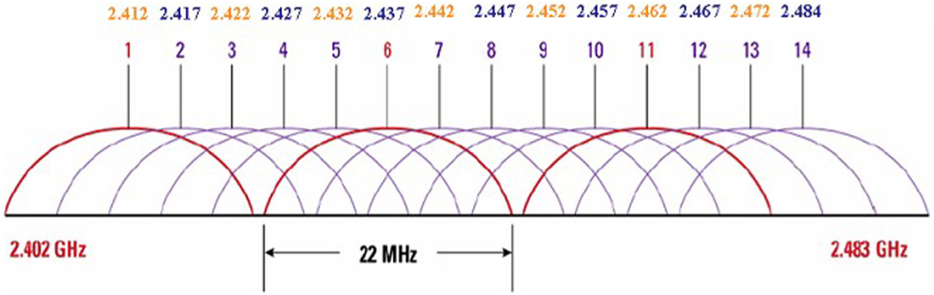
802.11n channel numbering.
Suppose that

Then, the time instant of frame header and frame tail are estimated as


After the acquisition of header and tail, the frame power (RSSI) is estimated by

The acquisitions of multiple frames are shown in Figure 7. The X-coordinate is samples, and the Y-coordinate is amplitude, which is scaled in mv. The time interval between adjacent samples is 50 ns, and the samples between the frames are noise. As we see, the time occupied by signal is much shorter than that occupied by noise. Figure 8 is a zoom in result of certain frame, where the signal is composed of a lot of samples. For the time interval gap is 50 ns, the frame is about 3.2 ms. Figures 9 and 10 depict the header and tail of a frame, respectively. The abscissa of Figures 9 and 10 denote the sample index, and the ordinate of these figures represent the measured amplitude of the waveform. The former part of Figure 9 is consisted of noise only, and the latter part of that is consisted of signal plus noise. In comparison, the former part of Figure 10 is consisted of signal plus noise, and the latter part of that is consisted of noise only. In our simulation, we set

Certain period of magnitude of sampled values.

Zoom-in of a frame.

Zoom-in of a frame header.

Zoom-in of a frame tail.
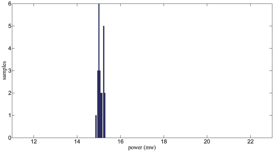
During 10 s, we have received 220 frames, and after the RSSI estimation of each frame, we interpolate the PDF curve in Figure 11. As we see, there are multiple peaks in the PDF curve. The first peak lies in the range of about [10 mw,13.5 mw], the second peak lies in the range of about [13.5 mw,16.5 mw], and the third peak lies in the range of about [16.5 mw,24 mw]. Before we seek for the reason of this phenomenon, we cut the 220 frames into three sections: the first 63 frames, the following 77 frames, and the last 80 frames. The histograms of the three sections are shown in Figures 12–14. As we can see, for different time durations, the RSSIs lie in different clusters, which means that there are some time-variant factors which have important impact on the RSSIs. Before we seek for the reason behind this phenomenon, we look at the histograms of the three sections versus the PDF of 220 frames, as shown in Figures 15–17. From these figures, we can see that different clusters of RSSI lie in different peaks of the interpolated PDF curves, different peak curves are similar. It can be inferred from the phenomenon that during a period of time, the transmit power, namely,

PDF interpolation of RSSI.
Histogram of the first 63 frames.

Histogram of the following 77 frames.

Histogram of the last 80 frames.

The histogram of the first 63 frames versus the PDF of 220 frames.

The histogram of the following 77 frames versus the PDF of 220 frames.

The histogram of the last 80 frames versus the PDF of 220 frames.
For each cluster, the PDF curve looks similar, but how can we prove it to be the same distribution. In this article, we should prove that the RSSIs satisfy a noncentral Chi-square distribution. We verify this from noncentral parameter of the Chi-square distribution. Namely, the calculated noncentral parameter from measured RSSIs should lie in the middle of the Chi-square distribution curve. First, we calculate the noncentral parameter of the first 63 frames by utilizing equation (25), which is 15.092 mw. The noncentral parameter lies in the middle of the peak as shown in Figure 18, which indicates that the RSSI values satisfy the property of noncentral Chi-square distribution. Furthermore, the noncentral parameters of the following 77 frames and the last 80 frames are given by 11.88 and 19.59 mw, which lie in the middle of their corresponding peaks as shown by Figures 19 and 20, respectively. It can be inferred from this phenomenon that the correctness of noncentral Chi-square distribution is verified from the aspect of noncentral parameter.

The calculated noncentral parameter based on the first 63 frames.
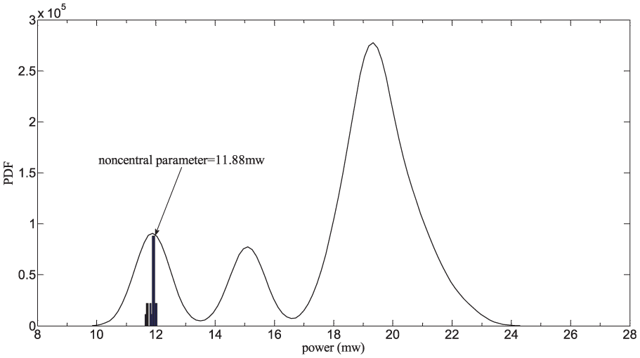
The calculated noncentral parameter based on the following 77 frames.

The calculated noncentral parameter based on the last 80 frames.
Conclusion
IEEE 802.11 WLAN (Wi-Fi) is an important tool to implement positioning in indoor environment as the signal of space information network, namely, GPS is unavailable therein, 20 and RSSI is the most prevalent parameter in the Wi-Fi-based indoor localization application. In this article, we first formulate the received signal in a multipath channel based on the IEEE 802.11 standard, then we derive the PDF of RSSI, and it is proved to be a noncentral Chi-square distribution rather than the Gaussian distribution.21,22 Finally, the correctness of the distribution is verified from the aspect of noncentral parameter in an experiment system. Given the statistical analysis and theoretical explanation, the design of indoor location sensing system could be more efficient and less time-consuming, and also the system performance such as accuracy and precision can be improved.
Footnotes
Handling Editor: Ota Kaoru
Declaration of conflicting interests
The author(s) declared no potential conflicts of interest with respect to the research, authorship, and/or publication of this article.
Funding
The author(s) received no financial support for the research, authorship, and/or publication of this article.