Sage Journals: Discover world-class research

Abstract

This article presents a novel distributed protocol for wireless sensor network formation and operation in multi-sink environments. It consists of three stages: the first one performs network formation and maintenance under a policy of low power consumption based on a local strategy in which every sensor node in the environment interacts only with the neighbour nodes. The second one uses local information to build trees from the sink nodes using a load balance strategy. In the third stage, the sinks collect sensed data through the trees. The protocol has been modelled by a timed Petri net, which is used first for a qualitative validation in which deadlocks, operational functionality, overflows, bottlenecks, and delays were checked, and later for network performance analysis.

Keywords

Wireless sensor networks multi-sink environments self-organization balanced trees Petri nets ZigBee protocol

Introduction

Wireless sensor networks (WSNs) are widely used in different kinds of applications, including intelligent buildings, environmental monitoring, surveillance and target tracking. Nowadays, this is an interesting trending research topic because of the complexity of problems dealing with diverse issues regarding the formation and maintenance of the networks, especially in the context of the Internet of Things (IoT) applications. Consequently, network reconfiguration (self-organization) in the event of failure of some nodes is a key and fundamental ability.

A WSN consists of a large number of low-powered and energy-constrained sensors. Sensor nodes are devices with limited energy resources, powered by a battery that in most cases it cannot be replaced once it is deployed. Despite memory and processing capacity operational constraints, sensors are expected to be functional, flexible and provide reliable results. Clusters are groups of devices usually managed by a node called Leader, Coordinator or Cluster Head (CH), which collects data from the member nodes in its cluster, aggregates the data and forwards it to the base station or sink.

Besides the challenge of defining efficient strategies for the formation and robust operation of WSNs, usual problems arise from the applications in real environments, namely the presence of obstacles, the quality of communication, the number of devices and the energy consumption. Another challenge is the handling of mobile nodes; the mobility of a node implies increasing the energy consumption and requires a better precision of the used location method, for example, a GPS, a triangulation strategy or even an extra device to control the movements of the sensor node. Additional emerging problems such as bad selection device, overhead, bottlenecks¹ and hotspot² arise from a bad network planning strategy. A combination of the best features of different strategies and algorithms can increase the network lifetime and meet the application requirements. For instance, in Rui and Wunsch,³ clustering is used for an effective solution to avoid the excessive energy consumption, and therefore, increasing overall network lifetime.

Related works

Recently, many works focus on reducing energy consumption or minimizing the number of hops. However, a route with the minimum number of hops may not always be the optimal and reliable route. The tree formation (TF) strategy is a known technique to reduce the overhead and the energy consumption; it also helps to create routes to send data through the network. However, a bad implementation of a TF can create deep branches, which becomes an inefficient way to send information; examples of these strategies were presented in previous studies.^4–8

Several works address the aggregation of data or data collection (DC) activities in the network; for instance, in Shrivastava and Pokle,⁹ a scheduling strategy to collect data in a WSN uses a TF algorithm. In this strategy, sensors are classified into different subsets; they are assigned to time slots as in the time division multiple access (TDMA) protocol. However, this scheme does not consider the energy consumption during the TF and the depth of a tree. DC schemes to minimize the overhead and excessive data transmission are presented in Tzong et al.¹⁰ and Yousefi et al.¹¹

One of the most popular cluster routing protocol in WSN is the low-energy adaptive clustering hierarchy (LEACH) presented in Heinzelman et al.¹² LEACH selects cluster heads with some probabilities; its goal is to reduce the energy consumption required to create and maintain clusters. However, cluster heads may be too close or too far from each other and this can affect the network performance. In Wang et al.,¹³ an energy routing strategy to extend the network lifetime based on a clustering technique is presented. This technique is an extension of LEACH, power-efficient gathering in sensor information systems (PEGASIS) and mobile-sink based energy-efficient clustering algorithm (MECA) algorithms.

Another important feature of WSN is data transport reliability. A survey of data transport reliability protocols is presented in Mahmood et al.¹⁴ Previous studies in WSNs have focused on the enhancement of network performance. Some works assume that there is a single stationary sink. In Carlos-Mancilla et al.,¹⁵ a tree-clustering strategy is used to collect data and forward it to a single node. However, a single sink serves as a single point of failure, making the network vulnerable to potential failures or attacks. A bio-inspired ant colony optimization algorithm (ACO) based on a clustering technique for home automation networking is proposed in Wang et al.¹⁶ A mobile sink communicates with every cluster head to collect data from the network. ACO is used to find the optimal route to the clusters. This proposal does not consider obstacles or transmission losses, or the depletion of energy.

In order to overcome the single sink problem, multi-sink networks are increasingly used. For instance, in Dandekar and Deshmukh,¹⁷ an energy balancing multi-sink optimal solution is presented. The objective is to find the optimal locations for every sink node to be placed as the centroid of every cluster. This is done by minimizing the average sensor distance between each sink and the sensor nodes and maximizing the one-hop connectivity. The proposal is based on particle swarm optimization (PSO) algorithm proposed in Kennedy and Eberhart;¹⁸ this scheme is centralized and the energy consumption is not considered in optimization method.

A distributed algorithm that builds a backbone connecting all mobile devices in an adaptive learning scheme for load balancing with a zone partition in a multi-sink WSNs (QAZP) is presented in Tzong and Chang.¹⁹ Although they propose a distributed strategy, the movement of the nodes is predefined, and failures and reconfiguration are not considered. A multiple data sink selection in a multi-sink environment is presented in Pietrabissa et al.²⁰ This algorithm works in a distributed and iterative manner, in which the sink role is periodically reassigned to avoid the hot spot problem and increase the lifetime of the network. However, this proposal does not consider the energy depletion in the topology formation nor in the overhearing problem.

Clustering schemes have been proposed for WSN formation. A clustering algorithm based on a self-organization strategy for ad-hoc wireless networks is presented in Olascuaga-Cabrera et al.;²¹ the goal is to save energy in order to increase the lifetime of the network and to keep all nodes connected as long as possible. This solution considers local decisions. Failures and loss of messages are not considered. In Hoang et al.,²² a framework that enables the development of a centralized cluster-based protocol for minimizing the inter-cluster distance between members and CHs is presented. It uses a harmony search algorithm (HAS), which is a music-based meta-heuristic optimization method.

Another global/centralized strategy for the formation and maintenance of a WSN is presented in Kim.²³ An automatically reconfiguration scheme for node failures in a multi-sink environment is also proposed. At an initial stage, nodes flood the system with messages to discover the best available route. The aim is to build a TF, using the received radio signal intensity.

In Lehsaini et al.,²⁴ a self-organization method is presented. The network is divided into clusters resulting in a hierarchical organization. Each sensor uses the residual energy and its k-density to elect the cluster head. The main purpose of this approach is to reduce the number of clusters. An initial cluster formation setup phase is performed and then a re-affiliation takes places.

In Xu et al.,²⁵ a clustering algorithm for multi-sink environments is proposed. Cluster heads are elected based on their residual energy. The routing protocol applies inter- and intra-clustering strategies in order to reduce energy consumption. The network is divided into N equal clusters and the data are forwarded to the corresponding sink. In the intra-cluster strategy, the cluster nodes forward data to the elected cluster head while inter-cluster strategy, this is done to the neighbour clusters heads. Energy consumption can be an issue since sinks are randomly located without any consideration.

The evaluation of two novel distributed clustering protocols is presented in Kumar;²⁶ the first one is a single-hop energy-efficient clustering protocol (S-EECP) in which the CHs are selected based on different weighted probabilities; the second one is a multi-hop energy-efficient clustering protocol (M-EECP) for heterogeneous WSNs in which it is assumed that all deployed sensor nodes are provided with different amounts of energy. In fact, this is considered a source of heterogeneity.

A localized algorithm for multi-sink networks is proposed in Carlos-Mancilla et al.²⁷ This algorithm includes three main stages. First, the backbone is built; in this stage, self-organization and clustering strategies are used by guaranteeing low energy consumption. In the second stage, trees are formed from the sinks using a load balancing strategy. In the third stage, sensor data are collected.

Most of the proposed protocols mentioned above only address a problem at once, namely routing, network topology formation, DC or reduction of energy consumption; besides, the proposals that include reconfiguration consume a lot of energy and resources. Additionally, many strategies are centralized, which implies that large-scale networks cannot be implemented in a short period of time without loss of reliability and functionality; on the other hand, distributed strategies do not provide enough information to improve their results.

Addressed challenges and summary of contributions

Network reliability and formation/routing for WSN are still active research areas. Some of the challenges in these areas include energy efficiency with minimal network overhead, routing redundancy and network reconfiguration.

An algorithm for formation and operation of WSNs is proposed; it includes three main stages. The first stage is the backbone formation (BF), which allows low energy consumption; it is based on self-organization and clustering techniques. In the second stage, trees are formed over the backbone; sinks devices are the root of such trees; the trees are formed by following a load balance strategy based on local information. Finally, in the third stage, sensed data are collected through the formed trees. During the network operation, disconnections are dealt and recovery procedures are applied.

The algorithm increases the lifetime of the whole network and reduces the number of transmissions, while provides an efficient way to collect data without loss functionality. This has been verified through simulation supported by MATLAB and a timed Petri net (TPN) model, which allowed representing the diverse concurrent procedures of the stages such as packet transmission and reception, and data processing. Experiments demonstrated lower energy consumption regarding that of the ZigBee protocol.

The main contributions include the following:

A reliable multi-hop multi-sink algorithm for network formation based on a self-organizing approach, which creates tree routes from the network formation.

A TF local strategy allowing load balancing.

A comparative analysis between ZigBee and the proposal regarding transmission and reception performance using a TPN model and a MATLAB program.

The remainder of this article is organized as follows: section ‘Background’ presents the Petri nets (PNs) basics and their application to performance analysis. Section ‘Network formation’ describes the strategies for network formation. Section ‘Networking with multiple sinks’ presents the TF and the sensor DC stages. Section ‘Protocol modelling’ presents the PN model. Section ‘Protocol assessment’ presents the quantitative analysis of the PN model and the ZigBee protocol. Finally, in section ‘Conclusion’, some concluding remarks are given.

Background

Timed PNs

We present the basic notions and notation of PNs and TPNs used in this article. For further information, please refer to Tadao.²⁸

Definition 1

A generalized PN N = (G, M) is a bipartite graph G with a marking function M. G = (P, T, Pre, Post, M), where:

P is a finite set of places (|P| = n ≥ 0),

T is a set of transitions (|T| = m ≥ 0), P ∩ T = Ø; P ∪ T ≠ Ø;

Pre is a previous incidence function which represents the weight of input arcs to transitions Pre: P × T → N^≥0; where N^≥0 denotes the set of non-negative integer numbers;

Post is a posterior incidence function (weight of output arcs) Post: P × T → N^≥0. Pre and Post are usually represented by matrices. Pictorially, circles are depicted as places, transitions as bars or rectangles, and arcs as arrows.

Places can contain tokens depicted as dots into the circles; the distribution of tokens in the net, called marking, is a function, M: P → N^≥0, usually represented by a vector [M(p₁) … M(p_n)]^T, where M(p_i) is the number of tokens in p_i; M₀ designates the initial marking.

The dynamic behaviour of a modelled system can be described by the evolution of the tokens along the net places. The evolution is controlled by a two-part rule:

A transition t_j ∈ T is enabled if ∀p_i ∈ P, M(p_i) ≥ Pre(p_i, t_j), that is, all its input places have at least as many tokens as the weight of the input arcs.

The firing (considered instantaneous) of a transition t_j may be performed if it is enabled. This invokes modification of the marking: every input place of t_j‘loses’ Pre(p_i, t_j) tokens and every output place of t_j‘gains’ Post(p_i, t_j) tokens. This is described by the following expression: M′(p_i) = M(p_i) – Pre(p_i, t_j) + Post(p_i, t_j) ∀p_i ∈ P.

Dealing with time in a PN, these elapsed times are assigned transitions or places. A combined qualitative and quantitative timed Petri net (TPN) to simulate the complete behaviour of a node in the algorithm described before is presented. In our model, the times are assigned to transitions; a formal analysis can be obtained according to the definition used in López-Mellado.²⁹

Definition 2

A timed transition Petri net (TTPN) is defined as (N, D, Γ) where D is a set of delays (or durations); D = {d_j} for j = 1,…, m, each d_j ∈ R^≥0 represents the time that a t_j takes to perform its firing, and Γ is an ordered set of elements (t_j, τ_k) ∈ T × R^≥0 representing the firing instant τ_k of a transition t_j, where R^≥0 denotes the non-negative real numbers. The firing of a transition t_j is performed as in PN with a slight variation: the tokens to be added in the output places appear after d_j time units. Transitions whose d_j = 0 are called immediate transitions.

WSN PN–based performance analysis

PNs presented in Tadao²⁸ are a graphical and mathematical modelling tool applicable to many systems. PNs are well suited to model systems with distributed, concurrent and asynchronous features, specifically TPNs proposed in Ramchandani³⁰ and taken up later by Popova.³¹

As a graphical formalism, PNs can be used as a visual communication similar to graphs, diagrams and networks. PNs allow modelling the behaviour of a node, simulating failures, and determining when a node is alive, as presented in Haddad³² and Zhou and Li.³³ The contribution of the PNs to model discrete event systems is well known. For instance, a method to analyse the behaviour of WSNs with a multi-hop architecture is presented in Lacerda and Lima.³⁴ Based on this, they are able to manage the delay time for arriving messages given a threshold and considering the data aggregation on intermediate nodes.

A graphical simulation system for modelling and analysis of sensor networks based on space time Petri net (STPN) and coloured Petri net (CPN) is presented in Yan and Tsai,³⁵ where a set of new concepts such as location, broadcast transition and dynamic topology is used to simulate the behaviour of a sensor network. In Sousa et al.,³⁶ a hybrid system formalism based on PNs to model the energy consumption of a sensor node is presented. A comparison between two different processor models in WSN based on Markov chains and PNs is proposed in Shareef and Zhu.³⁷ Results show that the PNs allow a much lower level of abstraction and closer to the actual implementation of the network. This research was extended in Shareef and Zhu.^38,39

When using PNs for system verification, it is possible to identify and detect failures during the design stage; then these can be eliminated, and therefore, the cost of debugging, maintenance and redevelopment can be significantly reduced.

The ZigBee protocol background

The WSNs formation includes both physical and logical organization issues. The IEEE 802.15.4-2006 is the most widespread and popular protocol to wirelessly interconnect low-cost sensors, actuators and processing devices. Compared to other protocols, it is the most efficient technology for sensor applications.⁴⁰

ZigBee supports network topologies such as peer to peer, star master–slave operation and clustered stars/tree topologies. The latter is used in distributed algorithms. The efficiency of this protocol in WSNs has been addressed in Abbagnale,⁴¹ Buratti et al.⁴² and Cuomo et al.⁴³ In this article, we address the simulation and analysis of the throughput of the ZigBee protocol and compare it to our proposal.

Network formation

The design of an efficient algorithm would be beneficial to obtain a better network performance. The proposed algorithm in Carlos-Mancilla et al.²⁷ is a combination of clustering and TF strategies. According to this algorithm, it is assumed that a determinate number of static nodes are randomly placed in a multi-sink environment without any apriori information.

A self-organized system is a set of autonomous devices with individual behaviour; this behaviour can be the same or different for all devices. The devices interact with each other to achieve a particular goal. The latter is a result of an emergent behaviour from the device interactions and coordination scheme. In general, individual behaviour derives from the execution of simple rules that evaluates local information and exchanges data with surrounding neighbours. Examples of these systems are found in nature, such as the foraging behaviour of ants (ACO algorithms) proposed in Dorigo et al.,⁴⁴ a school of fish presented in Schmeck et al.,⁴⁵ and from Mamei et al.⁴⁶ a biological cells inspired algorithm which achieves tasks with exceptional robustness, despite harsh and dynamic environments.

Clustering

Cluster head selection is based according to the needs of an application. For instance, a multi-criterion optimization to save energy and cluster formation technique is presented in Aslam et al.⁴⁷ The authors combine metrics to select the optimal cluster head node.

Our proposed clustering strategy, addressing the features described in Aslam et al.,⁴⁷ consists of selecting leader nodes with the highest weights taking into account the following parameters: residual energy and the number of neighbours Neighs of a node. Weight_i = E_res_(i) × Neighs_(i), where E_res = E_act – (E_TotaTx + E_TotalRx + (E_proc)); E_act is the actual energy of a node i before any processing has taken place; E_TotalTx, E_TotalRx and E_proc are the consumed total energy for transmissions, receptions and neighbour packet data processing in one iteration, respectively. The iteration consists of the different actions that a leader node can perform such as packet transmission and reception, neighbour packet data processing (data aggregation, info/data analysis) and active link verification in a given period of time. Weights are updated at the beginning of each iteration. The rest of the nodes, called cluster members, do not transmit their gathered data directly to the sink, but to their cluster head node.

Backbone formation strategy

In Carlos-Mancilla et al.,²⁷ every node i is identified by a unique ID and it is registered in a neighbourhood table. During the self-organization strategy, a node can play different roles: leader, member, gateway and bridge; these are shown in Figure 1. We propose an improved way of choosing a network role as described in Algorithm 1. Initially, the nodes do not have any role and all nodes are potentially able to become a leader, all nodes transmit a broadcast message (Hello message) for neighbourhood discovery within a coverage range and waits for a response from the neighbour nodes (Acknowledge message). The node which has the highest Weight_i value is selected as the cluster leader. This process is looped up to r-roles times. The self-organization process ends after this loop. The node verifies if there exists at least one neighbour in its neighbour table (Neightable) to start the selection of the role. The RoleF variable represents the role of the node during the BF. It is initialized to zero, representing that any role has been assigned yet. All changes are counted using variable nchanges.

Figure 1.

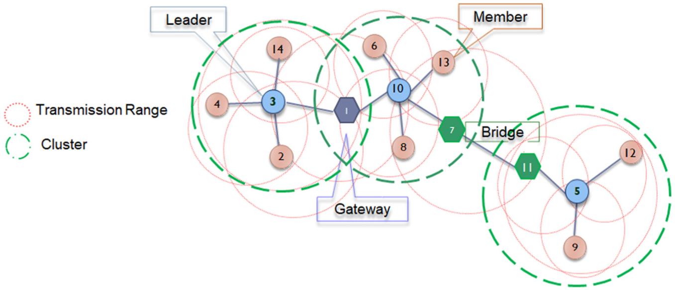
Network clustering.

Algorithm 1. Self-organization strategy.
RoleF ← none, nchanges←0 While (nchanges < r-roles) then // the node verifies a maximum threshold of no changes in the role value OldRoleF←RoleF If Neighs > 0 then //the node verifies there is at least one neighbour If Leaders = 0 then // there is no any leader node in their coverage area RoleF ₌ LEADER Else //there exist at least one leader If RoleF = LEADER then solve_conflict(); Else //the role is not leader If Leaders =1 then RoleF ← MEMBER verify_inconsistency(); Else //there exist more than one leader RoleF ← GATEWAY End if Bridge_nodes(); End if End if If OldRoleF != RoleF then nchanges ++ End if End if End While

Algorithm 1. Self-organization strategy.

RoleF ← none, nchanges←0
While (nchanges < r-roles) then // the node verifies a maximum threshold of no changes in the role value
OldRoleF←RoleF
If Neighs > 0 then //the node verifies there is at least one neighbour
If Leaders = 0 then // there is no any leader node in their coverage area
RoleF ₌ LEADER
Else //there exist at least one leader
If RoleF = LEADER then
solve_conflict();
Else //the role is not leader
If Leaders =1 then
RoleF ← MEMBER
verify_inconsistency();
Else //there exist more than one leader
RoleF ← GATEWAY
End if
Bridge_nodes();
End if
End if
If OldRoleF != RoleF then
nchanges ++
End if
End if
End While

The variable r-roles stores the current role of a device; if this variable changes its role more than once during the execution of the self-organization procedure and nchanges variable contains the maximum number of allowed role changes in one device; in this proposal, nchanges is set to three. OldRoleF and RoleF are the roles during the network formation stage, respectively. LEADER, MEMBER, GATEWAY and BRIDGE are the roles that a node can play during the network formation strategy; for more details, see Carlos-Mancilla et al.²⁷Weight_i is computed through an equation that measures evaluate which device with higher possibilities to be the cluster leader; the parameters to consider are the higher number of neighbours (Neighs) and energy (J). Whenever there is a conflict during the selection of a leader the solve_conflict() function is called. This occurs when two or more nodes have the same Weight_i value. The solve_function() compares the values of Weight_i from the participant nodes and decides which one will be the leader based on the minimum number of hops to the nearest sink node, the minor transmission range or the minor ID.

Another important function is verify_consistency() which prunes the unnecessary links and selects which node is chosen as a gateway (Figure 2); this can happen when two or more nodes connect the same clusters; thus, this function decides what node will be named gateway, based on the minimum number of hops and the level of energy. Finally, function Bridge_nodes() detects alternative communication links to assign the bridge role to join two segments of the network when it is required. For this purpose, the function verifies the existence of more than one different leaders through its member nodes neighbours; if some member neighbour has a different leader, both members become bridges.²⁷

Figure 2.

Gateway conflict solution: (a) two gateways want to connect the same pair of cluster and (b) solve_conflict function is performed.

An example of the solve_conflict() function is presented when two or more gateways want to connect the same pair of clusters (Figure 2(a)); the most potential node to become a gateway wins the connection and the other node withdraws its role to become a member (Figure 2(b)).

Once the BF has finished (called stabilization phase), all cluster members have to notify the end of the role assignment process ( Algorithm 1 ) to its leader node transmitting a stop message (stop_msg). When the leader receives the stop_msg from all its neighbours, it transmits a broadcast message (Endnottice) letting all members know that the BF is over, every node in the cluster must acknowledge this message. When that happens, they wait for level_message from the sink node to start the next stage called TF.

Networking with multiple sinks

The fault management, configuration and performance management (reduction of the number of transmissions, delays, scheduling and overhead control) are issues addressed in this section. The formation of the trees (network configuration) is performed following a distributed technique. A single sink scenario can be inefficient when there is a lot of information to handle, the network density increases, the transmission requests increase, the sink node is susceptible to failures and so on. If the network is not prepared for these changes, it will stop the operation;²⁷ furthermore, a multi-sink environment is presented.

The main benefits of the proposal are information redundancy, a regulated energy distribution and the load balance during TF. The stated problem consists of the formation of trees over the BF in which a group of designated nodes (sinks) will collect the data corresponding to sensor measurements and perform simple computation during the collection process.

Building the sensor trees

The number of placed sink nodes (k) can be defined by the application, usually, 2 ≤ k ≤ 4.¹⁷ The sink nodes have level 0 and they are the roots of the trees.

Every node has a table to keep the corresponding level for each sink in the network; this table is global and can be accessed at any time in the procedure as well as the received message (rx_packet). The level assignment procedure is described in Algorithm 2. The TF strategy waits for an incoming message to start the procedure and it is iterated until the node has no more changes in the level assignment value (r-times).

Algorithm 2. Tree formation strategy.
Level ← none, nchanges←0 While (nchanges ≤ r-times) then//the procedure ends when there are no more (r-times) level changes OldLevel←Level If Level > 0 then //Verify for the received level Level-assignment (); Else If Level = 0 then //assign level for the first time If rx_packet.Role ₌ LEADER or GATEWAY then Level ← rx_packet.level +1 Assignment_verification(); Else //Bridge Exception If rx_packet.Role = BRIDGE then Exception(); End if If OldLevel != Level then nchanges ++ End if End if End While

Algorithm 2. Tree formation strategy.

Level ← none, nchanges←0
While (nchanges ≤ r-times) then//the procedure ends when there are no more (r-times) level changes
OldLevel←Level
If Level > 0 then //Verify for the received level
Level-assignment ();
Else
If Level = 0 then //assign level for the first time
If rx_packet.Role ₌ LEADER or GATEWAY then
Level ← rx_packet.level +1
Assignment_verification();
Else //Bridge Exception
If rx_packet.Role = BRIDGE then
Exception();
End if
If OldLevel != Level then
nchanges ++
End if
End if
End While

When a node receives a message for the first time from the leader and the leader has already a level, the node will update its level and record it using the Assignment_verification() procedure, this function verifies which sink has already sent the level, the level is stored in the sink table. The node is stored if there is a change in the level assignment (OldLevel) during the iterations. When the node has already a level, and receive a lower one, the Level-assignment() function will verify if the received one is better than the current one; to verify if a level i is better of a level j, the node verifies the level is lower for at least two hops of difference. If the level j is better, the level i takes the value of the level j + 1 (level_i ← level_j + 1); also in this function, a new role is assigned; this procedure is explained below. For definition, a bridge is not able to assign a level except with one condition, evaluated with the Exception() function; such exception performs the following steps:

A bridge node i sends a message with its level to its other neighbour bridge j.

Node j keeps the received (level +1), builds a new message and sends it to its leader node.

The leader node compares its actual level with the received level +1 (rlevel), if it is lower, then the level of the leader and bridge j are reassigned; otherwise, the level is rejected.

An example is presented in Figure 3.

Figure 3.

Bridge assignment exception.

During the level assignment period, when a node has a level already assigned, a new role is assigned, which is stored in the RoleT variable; the considered role to DC stage is one of the following two roles:

Intermediate nodes (Int-node): this role is only given to the leaders, gateways and bridge nodes which have children nodes.

Leaf nodes (L-node): these nodes always have predecessor nodes and they do not have children, their previous role used to be a member node or a bridge.

Figure 4 shows an example of the level assignment procedure. The main objective of the TF stage is to achieve the load balance, distributing it among the deployed sinks, and to obtain the minimum number of hops to the nearest sink.

Figure 4.

Level assignment.

When some conflict arises during the level assignment, a verification process is executed to determine the node that will become the predecessor node, based on parameters such as the number of children, the number of hops to get to the nearest sink and the residual energy. An example of the conflict process and final TF is illustrated in Figure 5.

Figure 5.

Tree formation process: (a) a conflict emerging in the tree formation process and (b) final tree formation with the conflict resolution.

After every sink node builds its tree (Figure 6), a stabilization stage is defined. Leader nodes wait for a stop message (emessage) from all its neighbours and transmit it to its predecessor node.

Figure 6.

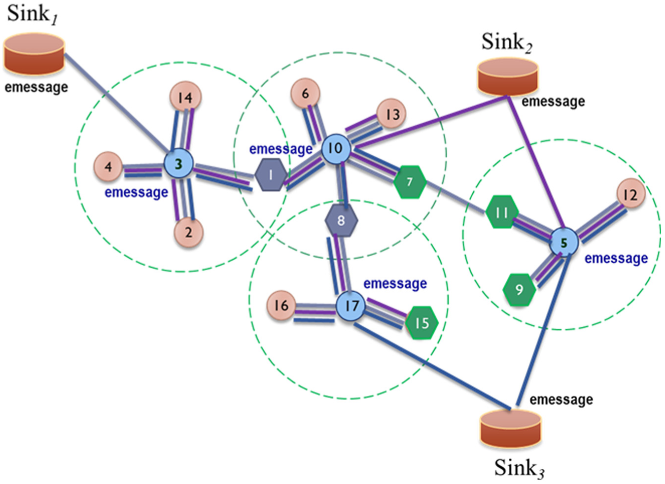
Every sink node builds its own tree and sends a stop message to its predecessor node.

The TF finishes when all sink nodes receive the emessage from all the local nodes connected. Once the level assignment is finished and the stabilization stage is successful, the Int-nodes (Gateways) become possibly cutting nodes.

Pruning strategy

Now it is necessary to define the conditions to perform the pruning of the tree by providing load balancing in an efficient way, and consequently reducing the energy consumption.

In Carlos-Mancilla et al.,²⁷ several rules for the pruning criteria were presented; in Algorithm 3, the pruning criteria are presented. The pruning strategy is repeated iteratively for the local number of pruning candidates. The algorithm operates according to its RoleF role. If the node has a Leader role, it sends a message to its neighbour nodes looking for more candidates to carry out a pruning; if one cluster has two or more gateways, they are added to the pruning candidates list. When the leader has more than two gateway neighbours and is near from the sink node (Level = 1), it will verify for redundant links (gateways that connect the same pair of clusters or gateways links that can be deleted).

Algorithm 3. Pruning strategy.
While (PruningCandidates=0) then If Role=Leader then Sendmsg(Boadcast); If Gateways >2 then// RULE 4- the leader has more than 2 gateways as neighbors Pruningcandidates(Gateways); End if If Gateways ≥ 1 and Level =1 then //RULE 3- one or more gateways and near of Redundant_links(); a sink node End if Else If Role= Gateway then // RULE 2- the node has more than two leaders with level 1 If Leaders>2 and Leaders.level=1 then Father_election(); End if Else If Role= Bridge then //RULE 1- The received level is lower at least two hops If (rx_packet.Level -2) < Level then Reassignment(); End if Else If Role=Sink then If leaders ≥ 2 then // RULES 5 and 6- The node verifies redundant links and decide the father Redundant_links(); election Father_election(); End if End if VerifyPruning_List(PrunCandidates); End While

Algorithm 3. Pruning strategy.

While (PruningCandidates=0) then
If Role=Leader then
Sendmsg(Boadcast);
If Gateways >2 then// RULE 4- the leader has more than 2 gateways as neighbors
Pruningcandidates(Gateways);
End if
If Gateways ≥ 1 and Level =1 then //RULE 3- one or more gateways and near of
Redundant_links(); a sink node
End if
Else
If Role= Gateway then // RULE 2- the node has more than two leaders with level 1
If Leaders>2 and Leaders.level=1 then
Father_election();
End if
Else
If Role= Bridge then //RULE 1- The received level is lower at least two hops
If (rx_packet.Level -2) < Level then
Reassignment();
End if
Else
If Role=Sink then
If leaders ≥ 2 then // RULES 5 and 6- The node verifies redundant links and decide the father
Redundant_links(); election
Father_election();
End if
End if
VerifyPruning_List(PrunCandidates);
End While

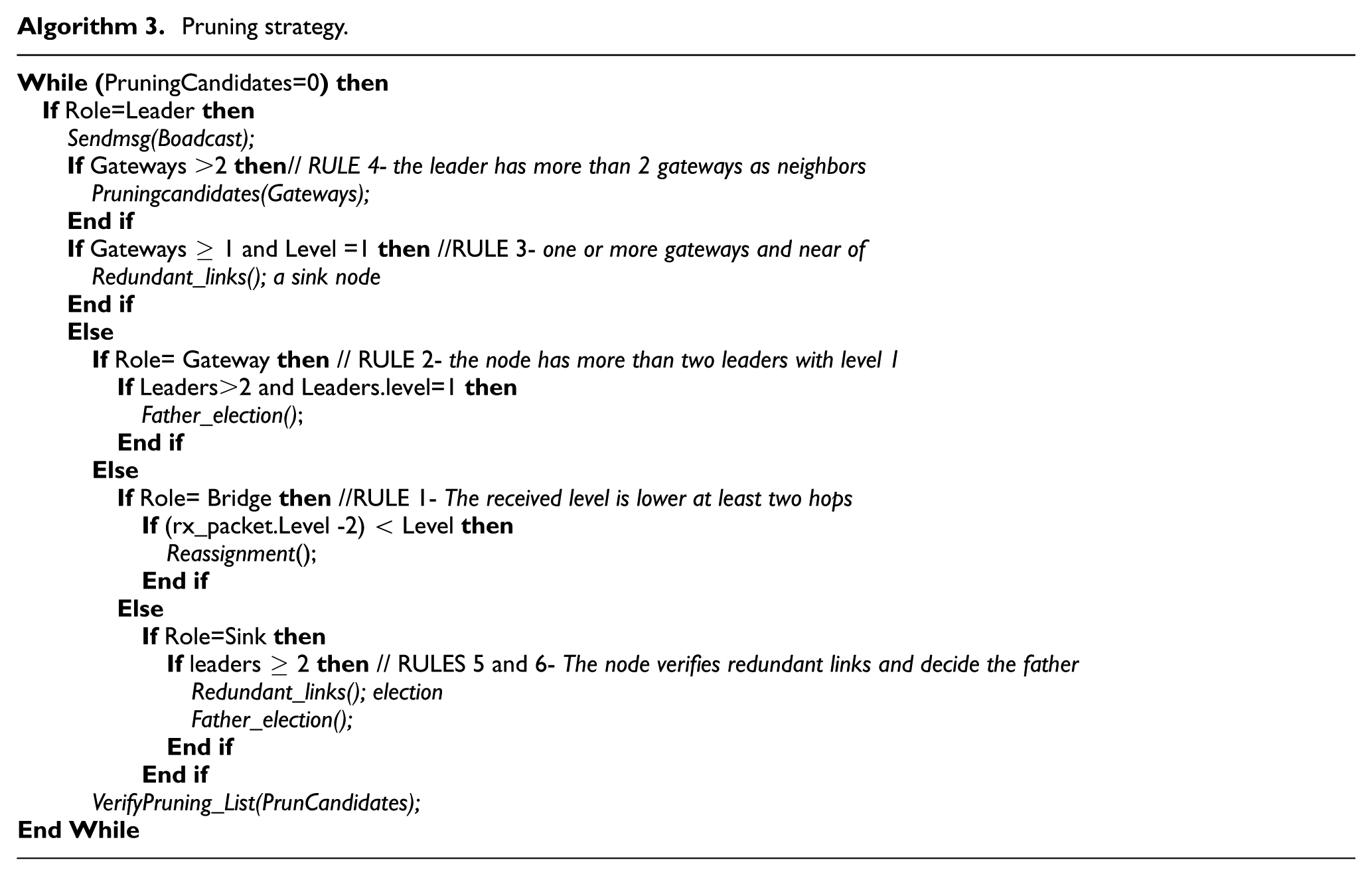
When the node is a gateway and it has two leaders as neighbours with level 1, the gateway will decide where the prune is made using the Father_election() procedure, which considers parameters such as a minimum number of children with every cluster, mayor residual energy, random ID and so on. If the node is playing the bridge role, then it is able to make a pruning if the rule exception explained in the TF stage occurs. Finally, a sink node is able to make a pruning when has more than two connections with a leader node. The leader node has to decide the pruning based on the father election parameters.

Each node compares the distance (level depth) to every sink in its sink table; it will choose as predecessor node, which provides the minimum number of hops to the nearest sink and the lower number of children.

The procedure is repeatedly executed as many times as necessary until there are no more pruning candidates (PrunCandidates) and all sink and member nodes have defined their predecessor nodes. Figure 7 illustrates the procedure previously described.

Figure 7.

Pruning strategy.

The TF procedure provides a load balancing of nodes distributed along the positioned sinks in the environment. Pruning decisions are local and hence cannot assure a global balancing. If there are no more changes, the sensing collection is performed. Figure 8 presents the result of the pruning algorithm.

Figure 8.

Final tree formation results.

Sensing and collection

Each node has a schedule to transmit/receive, sense and observe its idle times. There are two ways for transmitting the information:

Every node senses data and transmits the data at every defined period of time (Figure 9).

Unexpected transmissions happen when a node detects some undesired event. This event is transmitted until it gets to the sink node. The sink node decides what to do with such event (Figure 10).

Figure 9.

Sensing and data collection.

Figure 10.

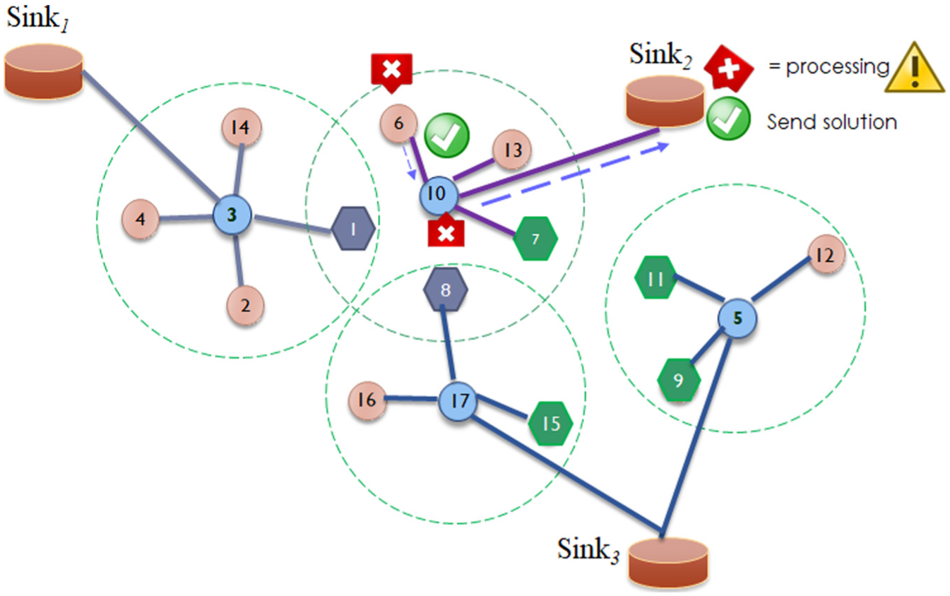
Unexpected event treatment.

The tasks for every role are presented in the following:

L-nodes: send its information to its father node.

Int-nodes: receive messages from all its neighbours, add its own data, process the information and send it to its father node until the data get to the sink node.

Sink node: processes and stores the information.

Nodes allow collecting and processing data by regarding energy saving, minimum hops, robustness and nodes maintenance. As noted previously, every node is able to perform all the activities, autonomously and independently to guarantee the communication with the other nodes using only local information. The overview of the complete networking process is given in Algorithm 4.

Algorithm 4. Overview.
Step 1: Each agent transmits a Hello message to nearby nodes (nodes inside a transmission range) to discover its neighborhood. Step 2: Once the transmitter agent receives an Acknowledge Message (ACK) as an answer, the self-organization starts. Step 3: When self-organization is over; each sink launches the tree formation algorithm, it means, each sink has at least one tree formation. Step 4: Int-nodes decide in which node the pruning is made. Step 5: Once the trees are set, each node transmits its information to its father node (preceding node) and so on, and then the information is collected by the assigned sink node.

Algorithm 4. Overview.

Step 1: Each agent transmits a Hello message to nearby nodes (nodes inside a transmission range) to discover its neighborhood.
Step 2: Once the transmitter agent receives an Acknowledge Message (ACK) as an answer, the self-organization starts.
Step 3: When self-organization is over; each sink launches the tree formation algorithm, it means, each sink has at least one tree formation.
Step 4: Int-nodes decide in which node the pruning is made.
Step 5: Once the trees are set, each node transmits its information to its father node (preceding node) and so on, and then the information is collected by the assigned sink node.

Protocol modelling

In this section, a TPN model of the protocol described in section ‘Networking with multiple sinks’ is presented. This model is used to validate the correctness of the protocol regarding the qualitative properties and also to evaluate its performance.

The PN model is first presented as modules describing the three stages of the protocol: BF, TF and sensing and DC; then the complete model is shown. Two parameters are fixed for simulation purposes: the maximum number of retransmissions is set to three, and the maximum number of neighbours of a node is defined as n_h = 6.

Model of the BF stage

Figure 11 shows the TPN describing the activities of this stage. Transitions depicted as white bars have a positive time assignment, while immediate transitions (fired as they are enabled) are depicted in black.

Figure 11.

TPN for the backbone formation stage.

In the model, the initial marking defines the idle state (P1), the maximum number of allowed changes in the role variable (P8), the maximum number of broadcast transmissions (P9) and the allowed number of incoming messages before being processed.

T1 represents the sensor initialization; then T2 models the broadcasting of the Hello message. The message arrival and acknowledgement are described by T10 and T3, respectively; the outcome of this process is adding a token in P3. T9 can be fired if there is not an incoming message (timeout); otherwise, with two tokens in P3, T4 is fired representing the message processing. T5 represents the updating of the agent role according to the self-organization procedure. Afterwards, if there is a communication with another node, the node stabilizes (firing of T6, T7 and T8) and reaches the initial state. The meanings of the places and transitions in this module are described in Table 1.

Table 1.

Conditions and functions in the BF stage.

Places	Transitions
P1 – initial state	T1 – turning on the sensor
P2 – condition for transmitting data	T2 – sending the Hello message
P3 – condition for receiving data	T3 – waiting for the Acknowledgement message
P4 – condition for registration process	T4 – registration process
P5 – condition to registration procedure	T5 – self-organization strategy function
P6 – condition for stabilize the stage	T6 – sending a direct message when the node has already communication with other node(s)
P7 – condition to finish the stage	T7 – sending the stabilization message
P8 – maximum number of role value change	T8 – ending the stage
P9 – maximum number of Hello transmissions	T9 – delay time for no arrivals messages
P10 – external event	T10 – receiving an incoming message
P11 – incoming messages

Model of the TF stage

The PN describing the TF strategy is presented in Figure 12. This procedure is outlined; tasks for Int-nodes (gateway and leader nodes) and L-nodes (member and bridge nodes) are separately presented. The node is able to perform the firing of sequences for either of Int-node or L-node.

Figure 12.

TPN for the tree formation stage.

The initial marking represents the condition to start the TF stage (P10) and the incoming messages (P13); afterwards, tokens in P14 indicate that a new message has been received; then the firing of T13 invokes the TF strategy function (Algorithm 2) to define the role according to the result of the previous stage (P13).

The sequence of activities for the L-node role are T17and T18, which defines the maximum number of iterations without changes in the level and the stabilization message, respectively. The firing sequence T14 T15 T16 defines the behaviour of an Int-node, which transmits its level, compares the levels with its neighbours and sends a message for stabilizing the stage if there are no changes. T19 represents the end of this stage and the beginning of DC stage. Table 2 describes in a concisely way the activities for this stage.

Table 2.

Conditions and functions in the TF stage.

Places	Transitions
P10 – starting the tree formation stage	T11 – tree formation message
P13 – incoming messages	T12 – incoming message
P14 – receiving data mode	T13 – tree formation strategy function
P15 – level assignment conditions	T14 – sending a message in Int-nodes
P16 – condition for sending a message in Int-nodes	T15 – comparative level changes procedure in Int-nodes
P17 – counting if there are level values changes in L-nodes	T16, T18 – ending the stage for Int-nodes and L-nodes, respectively
P18 – counting if there are level changes in Int-nodes	T17 – comparative level changes procedure in L-nodes
P19 – condition to stabilize the stage	T19 – stabilization stage; the DC is able to start

DC: data collection.

Model of the sensing and DC stage

Several transitions are fired by asynchronous external events, which represent requests or commands, such as sending packet requests, an external clock interruption or an unexpected packet arrival.

DC and sensing activities are modelled in the TPN in Figure 13; the initial marking in P20 represents the state in which a node is able to start the sensing and collection either for the L-nodes (T20) or Int-nodes (T21) roles. Places P30 and P31 are used to interconnect with the TF module. The latter represents the arrival of external events. The activities which do not depend on external events detection are described in the following.

L-node: the node senses the environment (P21), saves the information and sends it to its predecessor node (T22); the node gets in an idle mode (P22) and finishes the transmission (T23); the node starts the process again until the node detects an external event represented by T28.

Int-node: the place P23 represents the sensing mode of the node; afterwards, the transition T24 represents when the node waits for messages from all its neighbours; when the node receives a message, this message is treated by a reception function represented in T25; once the node has received the last message from its neighbours, the adding data procedure is represented by T26. Processing data mode is represented by the node in P26, and finally, the node transmits its own message to its predecessor node (T27). This process continues for a defined time or until some external event is detected, represented in T29.

Figure 13.

TPN model of the node; sensing and data collection.

Whether a node regardless of its role detects an event, the node performs a transmission (T28) to its predecessor node by a direct message represented in T30, then it waits for an Acknowledgement message from the node responsible for performing an activity to remove or solve the event (T31); once such node has handled the event, it returns to the idle state (T32). Table 3 describes the meaning of places and transitions in this TPN model.

Table 3.

Conditions and functions in the DC stage.

Places	Transitions
P20 – data collection stage initialization	T20, T21 – L-node and Int-node role tasks, respectively
P21, P23 – sensing mode for L-node and Int-node, respectively	T22 – transmitting data in L-nodes
P22 – idle mode in L-node	T23 – ending a transmission in L-nodes
P24 – counting the number of neighbours in Int-nodes based on the Neightable	T24 – count the total number of neighbours in Int-nodes
	T25 – receiving data in Int-nodes
P25 – comparison of the received data in Int-nodes	T26 – data aggregation procedure in Int-nodes
P26 – processing mode in Int-nodes	T27 – transmitting data in Int-nodes
P27 – incoming messages of neighbours in Int-nodes	T28, T29 – event detection in Int-nodes and L-nodes, respectively
P28 – transmission mode after an event detection	T30 – sending a direct message procedure after an event detection
P29 – reception mode after an event detection	T31 – acknowledgement received messages
P30, P31 – external events	T32 – returning to the normal procedure

The complete model

The complete model is shown in Figure 14; it is the composition of the PN models described above. Additional places and transitions (P38, P39, P40, T44, T45, T46 and T47) have been added to represent the interaction between stages of the protocol and to ensure the complete behaviour of a sensor node (Intermediate or Leaf). After executing the procedure of role assignment during the BF, in P40, the conditions to ensure the correct election of the new role are evaluated, both for Leaf (P38) and Intermediate (P39).

Figure 14.

Timed PN of the protocol. Screenshot of the qualitative analysis.

Transitions T46 (Member/Bridges) and T47 (Gateway/Leader) are responsible for executing the activities corresponding to the role value. There are two transitions used to return to the initial state; these are T45 for Leaf nodes activities and T44 for intermediate activities.

Timed transitions represent the duration for the transmission, reception and processing times. These times are set in an independent fashion along the PN model considering t time periods given by 0.3 ms < t < 2 ms. These times are based on ZigBee protocol features. The event detection (T28 and T29) in the model was set to every 2 ms.

The model has been tested using the PiPe v4.3.0 tool;⁴⁸ every stage was tested separately, without considering failures; the complete PN is bounded, cyclic and deadlock-free; Figure 14 shows a screenshot of the tool when the model was tested.

Protocol assessment

In this section, the proposed protocol is evaluated and compared to the ZigBee protocol; key features and performance are considered. The performance of successful transmitted and received messages is evaluated through the PN using the timing parameters of the ZigBee protocol.

ZigBee parameters

The timed parameters considered in the PN model are those used in the ZigBee protocol: the maximum payload is defined as (B) = 72 bytes, radiofrequency (RF) baud rate (802.15.4, 2.4 GHz) = 250 kbps, the Byte time at 250 kbps = 32 ms and the average total time for broadcast transmission of 64-bit is 0.8 + 0.032 Bms = 3.104 ms.

Considering the worst case for a broadcast transmission, we set 9.408 ms, and for the best case is 0.576 ms. The time for receiving an Acknowledgement message is 0.864 ms, the time to change between sleeping and active modes is 15 ms. The maximum number of retransmissions according to ZigBee protocol is three.

Time parameters are often presented with symbols used in the ZigBee protocol. These symbols can be converted to seconds by dividing the radio symbol rate settled to 62,500 symbols per second.

The maximum supported MAC layer payload is defined by aMaxMACFrameSize in the following formula

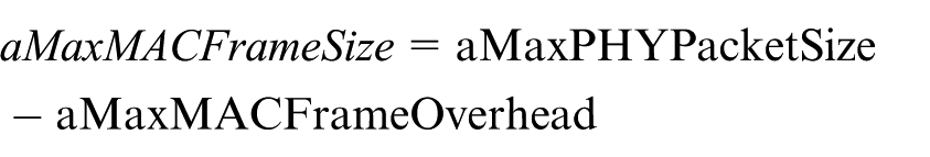
\begin{array}{l} a M a x M A C F r a m e S i z e = aMaxPHYPacketSize \\ - aMaxMACFrameOverhead \end{array}

where aMaxPHYPacketSize is the maximum size allowed for the packet in the physical layer and aMaxMACFrameOverhead is the maximum size of the packet in MAC layer. Then, we can obtain the times and number of received messages from the model which completes the parameters to calculate the throughput of the PN model and compare them with the ZigBee features. The calculation of the throughput for the evaluation of our model is given by

Throughput = \frac{(Tota l_{sendpackets} \times payload)}{T_{TxTime}}

where Total_sendpackets is the total number of packets sent and T_TxTime is the total transmission time.

Networking strategy

It is an interesting feature to compare the network strategies formation both the proposed protocol and ZigBee;⁴⁹ it is discussed below. ZigBee has three different roles for the devices, described below:

PAN coordinator (personal area network) acts as a router and manages the network load; it has all the functionalities of an FFD device. This node acts as a sink in a tree topology or network coordinator.

FFD (full function device) is able to perform any task such as communicating with all devices, transmitting, receiving and coordinate the communication.

RFD (reduced function device) is limited to the star topology; nodes communicate only with the network coordinators; they cannot play the role of network coordinator. These are simple devices with limited resources and communication requirements. They can only communicate with FDDs devices.

In Cipollone et al.,⁵⁰ a topology characterization analysis of an IEEE 802.15.4 multi-sink network is presented. Two scenarios are analysed in which the sinks are distributed along the proposed area. The first scenario considers the sinks inside the area, and the second one distributes the sinks around the environment. The authors define scenarios using 1, 9 and 49 sinks. The simulations halt when a sink is not able to detect an event and a path is defined as unusable when at least a node in the path dies due to the exhaustion of its energy. The route is defined by the positions of the source and destination in the tree. If two or more packets of one sensor have to be sent using the same tree, they can be aggregated in one packet. The simulations show that a scenario with less number of sinks is more efficient with a longer lifetime (scenario 1).

The reported simulations reveal several drawbacks: the complete connectivity of the network is not assured, sensors consume energy all the time since they assume that the sleep mode is not present; also they assume the packet reception is always successful and reconfiguration is not considered. The main differences between ZigBee and the proposal are described as follows.

The proposed protocol does not include a collision avoidance method such as ZigBee. The algorithm controls the number of transmissions allowing retransmitting any messages at most three times. The ZigBee protocol is able to use a peer to peer topology or even make a cluster-TF using predefined devices, while in the proposal the leader of the cluster can change its role when a device is no longer suitable to play it; even any member of the cluster is a candidate to take the leader role. Besides, ZigBee defines two roles for the devices and two different codes for each role and the topology created is centralized, in the proposal the code is the same for all devices and it is a distributed algorithm, the activities are set to four roles using local information Gateway, Bridge, Leader or Member (self-organization procedure).

The routing in IEEE 802.15.4 is defined according to a hierarchical structure, PAN devices receive the messages every period of time while all nodes listen to the entire environment, and the structure of the devices is defined according to the position of the node in a tree or in the formed cluster; also, the data aggregation is controlled by the PAN coordinator. Reconfiguration is not considered.

In the proposal, the routing is defined according to the cluster-TF considering the minimum number of hops to the closest sink. The formed trees consider also the level of the nodes and the number of children in every tree, which helps to improve the data collected from the sink nodes and balance the load between the available trees. Sinks are deployed at the beginning of the network in the defined monitoring area inside and around the environment. For the data aggregation, the member nodes send the sensed information every defined period of time, leader waits for a message from its neighbours and send only one packet with the collected information to the sink node. Also, the proposal considers reconfiguration.

In addition, several similarities can be pointed out: protocols save energy during the operation; they perform a cluster-tree topology, and both protocols may attempt until three transmissions when there is a problem in the reception (indeed in our protocol this number can be modified). These features were simulated in the proposal to measure a node response in a distributed scheme by considering the timing parameters and data features of ZigBee.

Performance evaluation

Besides the qualitative analysis of the protocol model provided by PNs, which allow determining properties such as deadlock-freeness and boundedness, the timed model provides a valuable simulation support and a reliable performance evaluation when the model represents real timing conditions. TPN is also useful for supporting what-if scenarios.

During the analysis of the proposed protocol, the timed parameters are associated with transitions to represent the waiting times of transmissions and receptions. The simulations of TPN provide a realistic analysis similar to Markov chain-type models;^37–39,51 however, the clearness of a PN model is better when it is necessary to describe concurrent activities and resource allocation.

In this analysis, the TPN is used to evaluate the performance of a node during its operation; the number of received messages and the number of transmissions can be evaluated. We consider the transmission times of the IEEE 802.15.4⁵² protocol to define the timing of transitions; the results obtained are similar to those of protocol in a node. Idle and sleeping times are too small; thus, they can be neglected in our procedure.

Two scenarios are considered: the first one evaluates the behaviour of the PN when the worst times are considered; the second one considers the best times in the PN model. The relationship between transitions and tokens is presented in Table 4.

Table 4.

Relationship between transitions, times and meaning.

Transitions	Description of the transition	Time (best times) (ms)	Time (worst times) (ms)
T8, T12	Incoming messages	0.0834	0.2502
T3	Acknowledgement messages	0.0834	0.2502
T9	Timeout time for Hello transmissions	9.408	3.104
T2, T22, T27, T6, T30	Transmissions	3.104	9.408
T2	Receptions	3.104	9.408
T28, T29	Event detection	2	2

Regarding the qualitative properties, a deadlock of the TPN model determines the connectivity of a node with any other node at any time. Boundedness implies that only one stage is executed at a time to ensure mutual exclusion control of events at any time within the node (a node is not able to transmit and wait for a message at the same time).

The simulations are based on MATLAB version R2013a⁵³ and a procedure developed for counting the number of successful transmissions and receptions. The tests are conducted using a payload of 72 bytes, with 100 simulations. Three scenarios were tested, in which the numbers of transmitted messages were set to 100, 200 and 500. The results are presented in Figure 15. In the graphics, the considered ZigBee theoretical throughput is presented with a red line and the performance of the proposed and PN modelled protocol is depicted with blue lines. Theoretical ZigBee throughput is based on ideal transmission and reception of messages; meanwhile, the strategy embedded in the Petri model considers timeouts, reconfigurations and retransmissions. The simulations consider the worst scenario in which there are three retransmissions and the cost of transmitting a message is the highest cost for transmitting messages.

Figure 15.

Multi-sink versus ZigBee protocol considering the worst scenario: (a) 100 transmitted messages, (b) 200 transmitted messages and (c) 500 transmitted messages.

The results shown in Figure 15 present a similar behaviour of our TPN model to ZigBee protocol. The transmitted messages during ZigBee simulations are almost 140 kb/s for all scenarios, in contrast to the simulation of the TPN model, whose value lies between 108 and 118 kb/s by sending a total of 100–500 messages. The worst operational scenario of the proposed and modelled protocol is reasonably close to the ZigBee ideal scenario.

In contrast, Figure 16 presents the behaviour of the PN model (proposed protocol) using ideal conditions of the environment without losses of messages, timeouts or reconfiguration. ZigBee defines a maximum of three attempts to send a message before to declare a loss in the transmission, receiving of failure to communicate a device with each other. In the best scenario simulations, neither losses nor jitter were assumed. These features are defined in the proposal to compare the behaviour of both strategies.

Figure 16.

Proposed model versus ZigBee protocol considering the best scenario: (a) 100 transmitted messages, (b) 200 transmitted messages and (c) 500 transmitted messages.

Note that the behaviour of the multi-sink protocol improves substantially the performance of the node compared to the worst scenario; the throughput is similar to that obtained by ZigBee on three different scenarios during the transmission of 100, 200 and 500 messages. The bytes transmitted using the worst scenario ranged from 105 to 120 kb/s; in the best scenario, the transmitted bytes fluctuate between 130 and 148 kb/s. The transmission rate using ZigBee protocol during simulations does not vary; it remains in 140 kb/s in the worst and the best scenarios, whereas the performance obtained by our proposed protocol increases significantly in all scenarios. Besides, the energy consumption is therefore reduced and the node lifetime is increased since the formation rules are driven by this. If we set the simulation with the best scenarios, the comparative is in many cases better than the ZigBee performance.

We present some simulations with Omnet++, using 14 randomly deployed static nodes and 3 sink nodes for clarity of the displayed information. All nodes execute the same proposed algorithm; Figures 17 and 18 show the communication process between the nodes in their transmission range. Figure 17 presents the backbone strategy; during this stage, the nodes send messages to the closest sensors to discover the neighbourhood. The grey circles around the nodes denote the communication range for every node. Figure 18 shows the transmitted messages between the nodes; in this process, it is possible to find messages such as Hello and AckHello messages, described in section ‘BF strategy’.

Figure 17.

Fourteen nodes and three sink nodes randomly deployed.

Figure 18.

Communication process.

Finally, Figure 19 presents the result of the roles assignment stage and the communication process. Regular nodes are presented in Grey, blue nodes are the leaders in the cluster, purple nodes are the gateways and grey nodes are the gateways. Grey circles denote the formed cluster. During a period, the formation remains stable transmitting regular messages between nodes to clusters and between the nodes to the closest sink.

Figure 19.

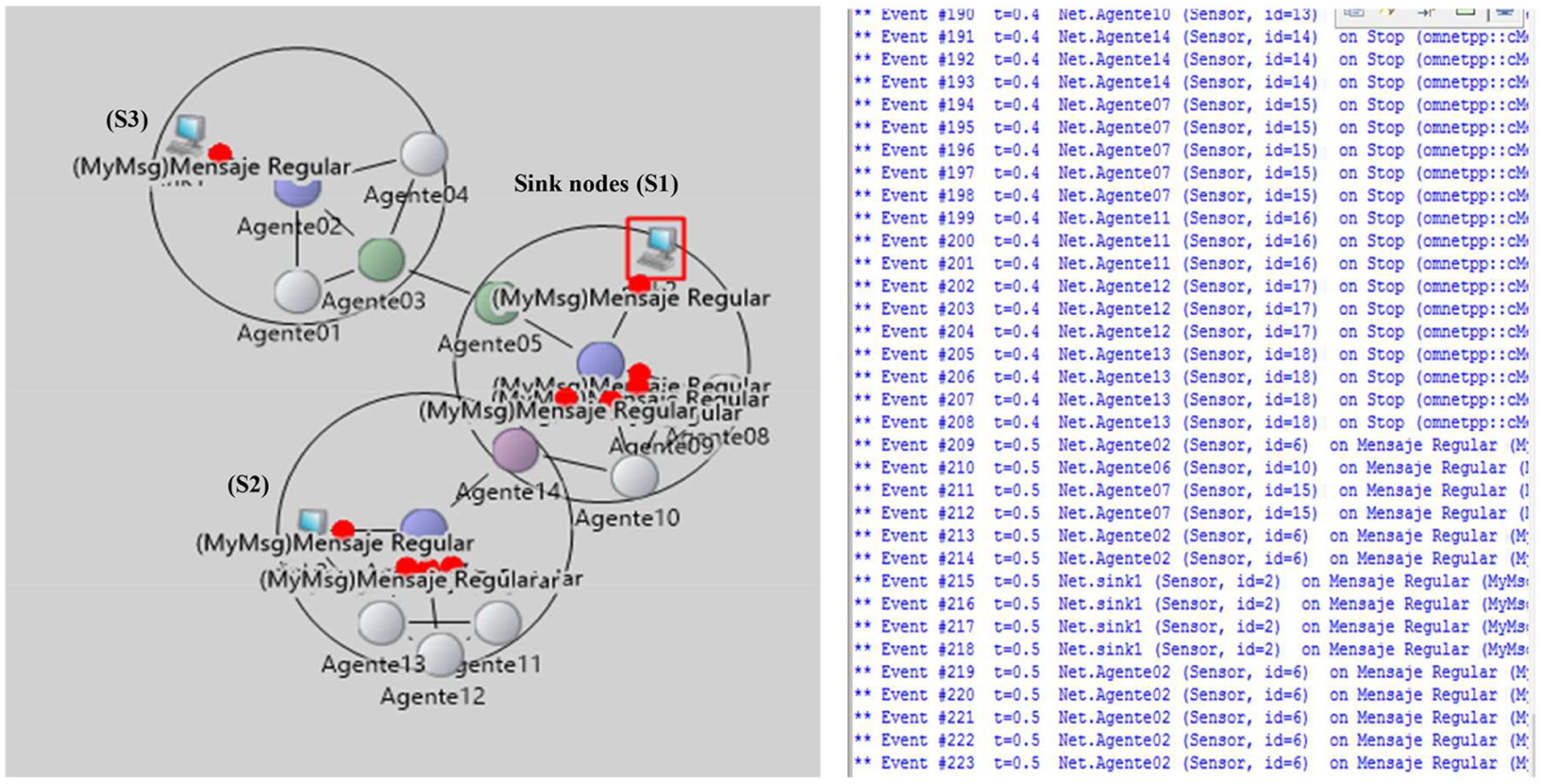
Topology formed during transmitted messages.

In this scenario, we can appreciate a similar network formation to that using ZigBee. One of the ZigBee topologies is a cluster-tree. The proposal considers a multi-sink strategy to distribute the load balancing between the available sinks and regulate the number of transmissions allowing reducing the consumed energy. According to the best scenario, our proposal consumes less energy increasing the lifetime of the network.

Finally, it is considered other scenario using 30 agents and 4 sinks in a square area of 1000 × 1000 m², as shown in Figure 20. In this scenario, some agents start sending a Hello message looking for neighbours and they do not have any role assigned. The simulation stops when all nodes are out of power; the agents are initialized with 100 J of energy, and a depletion of 1 J for transmission and reception. The considered delay is set to 100 ms and a range of transmission of 100 m.

Figure 20.

Scenario using 30 agents and 4 sink nodes; agents are looking for neighbours.

Different stages of simulation are presented in Figure 21. As shown in Figure 21(a), agents transmit and receive Hello and Acknowledgement messages to discover the neighbourhood; as shown in Figure 21(b), nodes have chosen their role divided into Leader, Gateway, Bridge and Member; only Leader and Gateway nodes show its energy level. During the simulation, the agents display the energy level every defined period of time, and when some change in the role or level has occurred. Finally, Figure 21(c) shows some important parameters from the simulation, such as the number of messages sent by every agent during the simulation, the simulation time, the number of generated events and some relevant information during transmissions such as ID, the number of neighbours, source and destination.

Figure 21.

Scenario with 30 agents and 4 sinks with 100 J of initial energy: (a) agents transmit and send Hello and Acknowledgement messages, (b) intermediate agents (Leader and Gateway) are defined and show its level of energy and (c) simulations parameters.

Results show a total simulation time of 804 s with a total of 16,599 presented events. The agents send different numbers of messages around the environment, between 600 and 1300 messages according to the role and the sensed information. The reported information shows the source and destination of some messages (some messages area), the id and the kind of the message. The network can be simulated using as many nodes as the environment can represent (100, 1000).

In this article, the maximum number of used nodes is set to nodes to appreciate the messages and information transmitted in the whole network, with more devices the information is not visible but definitely can be obtained.

Conclusion

The presented protocol considers the inherent problems to WSNs, which are the constraints of energy and memory; it provides a set of strategies that achieve a successful communication for every stage (Network Formation, TF to control de transmissions, DC and Reconfiguration), which increases the lifetime of the whole network. Every proposed stage specifies a set of distributed and local activities.

The formation of the trees considers a load balancing of nodes, which make an efficient DC. Every intermediate node (leader, gateway) waits for messages from all its neighbours to send the data through the tree until the closest sink, which reduces the energy consumed by sending only one message and therefore increasing the lifetime of the whole network.

The proposed scheme allows controlling the number of transmissions, reducing the delays and increasing the performance. It also reduces the energy consumption and includes routing, reconfiguration and network formation strategies.

The solution involves a self-organization strategy in network formation; afterwards, the TF strategy uses local information and builds the load-balanced trees over the formed network in a multi-sink environment and finally, sensing and DC process are executed at every defined period. The presented algorithm allows addressing challenging problems inherent to wireless sensors such as energy consumption, memory, latency, loss of messages, routing and the number of retransmissions that affect the performance of the whole network.

A TPN model has been useful to formalize the behaviour of the algorithm and to verify liveness, deadlocks freedom and home state properties. These properties guarantee the availability of the sensor devices during the whole process, the robustness and reliability during the communication. Besides, the reconfiguration case when the device has to redo the procedure has been clearly represented.

An evaluation based on the features of the IEEE 802.15.4 model is presented. Simulation experiments demonstrate that the presented protocol behaves better or similar (in the worst-case situations) than the ZigBee protocol allowing a good energy saving. The strategies used in this article extend our previous works to deal with multi-sink environments since simulation experiments confirm the best performance regarding energy consumption and operation efficiency. Consistent with the distributed nature of the protocol, the load balancing stage is also distributed and localized, in contrast to ZigBee, which uses global knowledge from the entire environment.

Future research deals with the ability of autonomous network reconfiguration in order to recover from situations in which sensors or sinks are lost. The current version of the proposed protocol only considers fixed static nodes deployed in random environments; it can be implemented in indoor or outdoor settings and tested on more dense scenarios (using up to 1000 nodes). In the future, the mobility of the nodes will be considered. The protocol can be implemented for surveillance, agriculture and forest monitoring, smart houses, health care, building facility management and similar applications where there are limitations on energy consumption, information management and the people access.

Footnotes

Academic Editor: Michele Amoretti

Declaration of conflicting interests

The author(s) declared no potential conflicts of interest with respect to the research, authorship, and/or publication of this article.

Funding

The author(s) disclosed receipt of the following financial support for the research, authorship, and/or publication of this article: This work has been partially supported by CONACYT, grant no. 243189 (M. Carlos-Mancilla).

References

Hochbaum

Shmoys

. A unified approach to approximation algorithms for bottleneck problems. J ACM 1986; 33(3): 533–550.

Sungjin

Kim

. Proactive context-aware sensor networks. In: Proceedings of European workshop on wireless sensor networks, Zurich, 13–15 February 2006. Berlin: Springer.

Rui

Wunsch

. Survey of clustering algorithms. IEEE T Neural Networ 2005; 16(3): 645.

Evangelos

Warnier

Brazier

FMT

. Adaptation strategies for self-management of tree overlay networks. In: 11th IEEE/ACM international conference on grid computing (GRID 2010), Brussels, 25–29 October 2010, pp. 401–409. New York: IEEE.

Singh

Lal

Sethi

et al . A tree based routing protocol for Mobile Sensor Network (MSNs). Int J Comput Sci Eng 2010; 1(Suppl. 1): 55.

Zhang

. DCTC: dynamic convoy tree-based collaboration for target tracking in sensor networks. IEEE T Wirel Commun 2004; 3(5): 1689–1701.

Zhang

. Optimizing tree reconfiguration for mobile target tracking in sensor networks. In: Twenty-third annual joint conference of the IEEE computer and communications societies (INFOCOM 2004), Hong Kong, China, 7–11 March 2004, vol. 4, pp.2434–2445. New York: IEEE.

Zhang

Wang

Liang

et al . Load-balancing routing for wireless sensor networks with multiple sinks. In: Proceeding of 12th international conference on fuzzy systems and knowledge discovery (FSKD), Zhangjiajie, China, 15–17 August 2015. New York: IEEE.

Shrivastava

Pokle

. Energy efficient scheduling strategy for data collection in WSNs. In: International conference on electronic systems, signal processing and computing technologies (ICESC), Nagpur, India, 9–11 January 2014, pp.170–173. New York: IEEE.

10.

Tzong

Zhang

Pan

. One handshake can achieve more: an energy efficient, practical pipelined data collection for duty-cycled sensor networks. Proc IEEE Sens J 2016; 16(9): 3308–3322.

11.

Yousefi

Malekimajd

Ashouri

et al . Fast aggregation scheduling in wireless sensor networks. IEEE T Wirel Commun 2015; 14(6): 3402–3414.

12.

Heinzelman

Chandrakasan

Balakrishnan

. Energy-efficient communication protocols for wireless microsensor networks. In: Proceedings of the 33rd Hawaii international conference on systems science (HICSS), vol. 8, Washington, DC, 4–7 January 2000. New York: IEEE.

13.

Wang

Cao

et al . An improved energy-efficient clustering algorithm based on MECA and PEGASIS for WSNs. In: Third international conference on advanced cloud and big data, Yangzhou, China, 30 October–1 November 2015, pp.262–266. New York: IEEE.

14.

Mahmood

Seah

WKG

Welch

. Reliability in wireless sensor networks: a survey and challenges ahead. Comput Netw 2015; 29: 166–187.

15.

Carlos-Mancilla

López-Mellado

Mendez-Vazquez

. Design and implementation of a Robust Wireless Sensor Network. In: International conference on electronics, communications and computers (CONIELECOMP 2013), 11–13 March 2013, Puebla, Mexico, pp.11–13. New York: IEEE.

16.

Wang

Cao

et al . Bio-inspired ant colony optimization based clustering algorithm with mobile sinks for applications in consumer home automation networks. IEEE T Consum Electr 2015; 61(4): 438–444.

17.

Dandekar

Deshmukh

. Energy balancing multiple sink optimal deployment in multi-hop Wireless Sensor Networks. In: Advance computing conference (IACC), Ghaziabad, India, 22–23 February 2013, pp.408–412. New York: IEEE.

18.

Kennedy

Eberhart

. Particle swarm optimization. In: Proceedings of IEEE international conference on neural networks, Perth, WA, Australia, 27 November–1 December 1995, vol. 4, pp.1942–1948. New York: IEEE.

19.

Tzong

Chang

. An adaptive learning scheme for load balancing with zone partition in multi-sink WSN. Expert Syst Appl 2012; 39: 9427–9434.

20.

Pietrabissa

Liberati

Oddi

. A distributed algorithm for Ad-hoc network partitioning based on Voronoi Tessellation. Ad-Hoc Netw 2016; 46: 37–47.

21.

Olascuaga-Cabrera

López-Mellado

Mendez-Vazquez

et al . A self-organization algorithm for robust networking of wireless devices. IEEE Sens J 2011; 11(3): 771–780.

22.

Hoang

Yadav

Kumar

et al . Real-time implementation of a harmony search algorithm-based clustering protocol for energy-efficient wireless sensor networks. IEEE T Ind Inform 2014; 10(1): 774–783.

23.

Kim

. Spanning tree based topology configuration for multiple-sink Wireless Sensor Networks. In: First international conference on ubiquitous and future networks (ICUFN), Hong Kong, China, 7–9 June 2009, pp.122–125. New York: IEEE.

24.

Lehsaini

Guyennet

Feham

. A novel cluster-based self-organization algorithm for wireless sensor networks. Sens Netw 2010; 7(1–2): 85–94.

25.

Yin

Wang

et al . An energy-efficient multi-sink clustering algorithm for wireless sensor networks. Int J Contr Autom 2012; 5(4): 34–39.

26.

Kumar

. Performance analysis of energy efficient clustering protocols for maximising lifetime of wireless sensor networks. IET Wirel Sens Syst 2014; 4(1): 9–16.

27.

Carlos-Mancilla

López-Mellado

Siller-Gonzlez

. A localized multi-sink multi-hop algorithm for Wireless Sensor Networking. In: IEEE global information infrastructure and networking symposium (GIIS), Guadalajara, México, 28–30 October 2015. New York: IEEE.

28.

Tadao

. Petri nets: properties, analysis and applications. Proc IEEE 1989; 77(4): 541–580.

29.

López-Mellado

. Analysis of discrete event systems by simulation of timed Petri net models. Math Comput Simulat 2002; 61: 53–59.

30.

Ramchandani

. Analysis of asynchronous concurrent systems by timed Petri nets. PhD Thesis, Massachusetts Institute of Technology, Cambridge, MA, 1974.

31.

Popova

. On time Petri nets. J Inform Process 1991; 27(4): 227–244.

32.

Haddad

. Time and timed Petri nets. ENS Cachan & CNRS & INRIA, DISC, June 2011, http://www.lsv.fr/∼haddad/disc11-part1.pdf

33.

Zhou

. Chapter 2: Petri nets. In: Li

Zhou

(eds) Deadlock resolution in automated manufacturing systems: a novel Petri net approach. Berlin: Springer, 2009, pp.17–43.

34.

Lacerda

Lima

. Petri nets as an analysis tool for data flow in wireless sensor networks. In: Proceedings of 1st Portuguese conference on wireless sensor networks, Coimbra, Portugal, 4 March 2011, pp.1–6. University of Coimbra.

35.

Yan

Tsai

JJP

. A graphical simulation system for modeling and analysis of sensor networks. In: Seventh IEEE international symposium on multimedia, Irvine, CA, 14 December 2005, pp.12–14. New York: IEEE.

36.

Sousa

JRB

Lima

AMN

Perkusich

. Modeling and analyzing power consumption in sensor networks nodes based on differential hybrid Petri nets. In: 31st IEEE annual conference of Industrial Electronics Society (IECON), Raleigh, NC, 6–10 November 2005, pp.6–10. New York: IEEE.

37.

Shareef

Zhu

. Energy modeling of processors in wireless sensor networks based on Petri nets. In: Proceedings of the 2008 international conference on parallel processing workshops (ICPPW ‘08), Portland, OR, 8–12 September, pp.129–134. New York: IEEE.

38.

Shareef

Zhu

. Energy modelling of nodes based on Petri nets. In: Proceeding of 39th international conference on parallel processing (ICPP), San Diego, CA, 13–16 September 2010, pp.13–16. New York: IEEE.

39.

Shareef

Zhu

. Effective stochastic modeling of energy-constrained wireless sensor networks. J Comput Netw Commun 2012; 2012: 870281.

40.

Gutierrez

Durocher

. On the use of IEEE 802.15.4 to enable wireless sensor networks in pulp and paper industry. In: Proceedings of the IEEE pulp and paper industry technical conference, Jacksonville, FL, 20–23 June 2005. New York: IEEE.

41.

Abbagnale

. A case study for evaluating IEEE 802.15.4 wireless sensor network formation with mobile sinks. In: IEEE international conference on communications (ICC ‘09), Dresden, 14–18 June 2009, pp.1–5. New York: IEEE.

42.

Buratti

Francesca

Luna

et al . Optimum tree-based topologies for multi-sink wireless sensor network using IEEE 802.15.4. In: 65th vehicular technology conference, Dublin, 22–25 April 2007, pp.130–134. New York: IEEE.

43.

Cuomo

Della Luna

Cipollone

et al . Topology formation in IEEE 802.15.4: cluster-tree characterization. In: Sixth annual IEEE international conference on pervasive computing and communications, Hong Kong, China, 17–21 March 2008, pp.276–281. New York: IEEE.

44.

Dorigo

Birattari

Stützle

. Ant colony optimization–artificial ants as a computational intelligence technique. IEEE Comput Intell M 2006; 1: 28–39.

45.

Schmeck

Muller-Schloer

Cakar

Emre

et al . Adaptivity and self-organization in organic computing systems. ACM T Auton Adap Sys 2010; 5(3): 10:1–10:32.

46.

Mamei

Menezes

Tolksdorf

et al . Case studies for self-organization in computer science. J Syst Architect 2006; 52(8): 443–460.

47.

Aslam

Phillips

Robertson

et al . A multi-criterion optimization technique for energy efficient cluster formation in wireless sensor networks. Inform Fusion 2011; 12(3): 202–212.

48.

Dingle

Knottenbelt

Suto

. PIPE2: a tool for the performance evaluation of generalised stochastic Petri nets. ACM SIGMETRICS Perform Eval Rev 2009; 36(4): 34–39, http://pipe2.sourceforge.net/

49.

Carlos-Mancilla

López-Mellado

Siller

. Wireless sensor networks: approaches and techniques. J Sensor 2016: 2016: 2081902.

50.

Cipollone

Cuomo

Della Luna

et al . Topology characterization and performance analysis of IEEE 802.15.4 multi-sink wireless sensor networks. In: Annual Mediterranean ad hoc networking workshop (MED-HOC-NET ’07), vol. 7, Corfu, Greece, 13–15 June 2007, pp.196–203. Publisher Ionian University.

51.

Silva

Del Foyo

PMG

. Timed Petri nets. In: Pawlewski

(ed.) Petri nets–manufacturing and computer science. Rijeka: IN TECH, 2012, https://www.intechopen.com/books/petri-nets-manufacturing-and-computer-science/timed-petri-nets

52.

IEEE 802.15.4-2006. IEEE standard for information technology – telecommunications and information exchange between systems – local and metropolitan area networks – specific requirements – part 15.4: Wireless Medium Access Control (MAC) and Physical Layer (PHY) specifications for Low Rate Wireless Personal Area Networks (LR-WPANs).

53.

MATLAB R13b, 2013, https://www.mathworks.com/products/new_products/release2013b.html

An efficient reconfigurable ad-hoc algorithm for multi-sink wireless sensor networks

Abstract

Keywords

Introduction

Related works

Addressed challenges and summary of contributions

Background

Timed PNs

Definition 1

Definition 2

WSN PN–based performance analysis

The ZigBee protocol background

Network formation

Clustering

Backbone formation strategy

Networking with multiple sinks

Building the sensor trees

Pruning strategy

Sensing and collection

Protocol modelling

Model of the BF stage

Model of the TF stage

Model of the sensing and DC stage

The complete model

Protocol assessment

ZigBee parameters

Networking strategy

Performance evaluation

Conclusion

Footnotes

Declaration of conflicting interests

Funding

References