
Abstract
Industrial cyber-physical system is defined as transformative technologies for upgrading the traditional industrial mode. Wireless mesh network becomes a typical technology in industrial cyber-physical system for the network communication with large-scale distributed wireless terminals. However, the robustness of wireless mesh networks in the industrial environment is seriously challenged by worst working reliability of network nodes, more vulnerable wireless communication links, and so on. In this article, in order to enhance network robustness and reliability, we propose a robust collaborative mesh networking method for interconnecting large-scale distributed wireless heterogeneous terminals in industrial cyber-physical systems. First, moderate redundancy of network deployment is introduced to guarantee two-connectivity for each mesh router and two-coverage for each wireless terminal, and an improved metric for evaluating the overall network robustness is presented. Second, the robustness-aware collaborative mesh networking problem is formulated with a multi-objective optimization model, and an improved multi-objective particle swarm optimization algorithm based on self-adaptive evolutionary learning is exploited to search out the Pareto optimal particles with better distribution and diversity. The experimental results show how the network robustness and load-balancing performance change along with the increasing number of deployed mesh router/mesh gateways, and our method is helpful for finding out a robust wireless mesh network deployment scheme in industrial cyber-physical systems when given a deployment cost.
Keywords
Introduction
Industrial cyber-physical system (ICPS) 1 is considered to be a core technology system for creating an advanced industrial mode by integrating the emerging information and network technologies (e.g. data sensing, industrial network, high-performance computing, intelligent decision-making, and controlling) with the industrial process. 2 Specifically, by integrating the following elements such as embedded systems, radio-frequency identification (RFID) tags and readers, sensors, actuators, and wireless networks in the whole industrial process, it is able to achieve dynamic data perception of various industrial resources (e.g. workers, materials, equipment, semi-finished products, products) and realize precise scheduling and controlling of the entire industrial process with intelligent data processing, computing, analysis, and decision-making. Based on the distributed collaboration of various sensing devices, computing equipment, and actuators, ICPSs will greatly improve the performance of the industrial manufacturing system on the following aspects including real-time interaction, fast response, efficient collaboration, dynamic optimization, and so on.
A typical device deployment example in ICPSs 3 is shown in Figure 1, and a great number of various wireless terminals (WTs) are widely used, usually including handheld RFID readers, personal digital assistants (PDAs), sensors, wireless industrial instruments, video cameras, controllers/actuators, and so on, which undertake the data perception, optimal scheduling, and controlling of a variety of objects (e.g. human, material, equipment, production process, products) in the whole industrial process. With the large-scale distributed heterogeneous WTs in ICPSs, it is much important to develop an efficient high-performance collaborative networking method, which is vital for achieving stable, reliable, real-time, and energy-efficient sensing and controlling data transmission.

A vertically layered mesh network in ICPSs.
The application of traditional networking solutions with the wired network or wireless access point (AP) is limited in the tough industrial environment,4,5 for example, higher deployment cost and construction difficulty with the wired network, communication blind spots, and single-point failure with independent wireless APs. In order to reduce network deployment cost and enhance network robustness, as shown in Figure 1, an improved networking method with a vertically layered mesh network topology is presented. The upper layer is the wireless high-speed backbone transmission network composed of multi-hop interconnected wireless mesh routers (MRs) over WiFi. Moreover, the MR is compatible with a variety of common communication modes, such as WiFi, Zigbee, Bluetooth, and support ubiquitous network accessing for kinds of WTs such as RFID readers, sensors, wireless industrial instruments, cameras, and controllers/actuators. The lower layer is the accessing layer which includes kinds of WTs, and each MR is responsible for managing a cluster of adjacent WTs, as well as their uplink and downlink data forwarding. Each WT supports multi-hop communication mode to provide network connectivity redundancy for network link failure. Meanwhile, in order to achieve real-time and reliable data transmission, the size of each cluster under the MR should not be too large, namely the maximal network hop of each cluster should be limited.
The network topology presented in Figure 1 is a typical and more complex wireless mesh network (WMN), which is becoming an important networking infrastructure due to their low deployment cost and robust wireless network connectivity. In WMNs, there are three types of mesh nodes: mesh gateways (MGs), MRs, and WTs. The MRs generally have higher communication and computation capacities, which are responsible for constituting the wireless backbone network and providing multi-hop network interconnection for distributed WTs, and some MRs (also called mesh gateways) are responsible for connecting with the wired network.
How to plan and construct a high-performance WMN has been widely concerned in recent years. 6 Typically, given a number of distributed WTs, the performance of WMNs is primarily affected by the deployment (e.g. location, number) of MGs and MRs, which plays an important role in achieving different properties such as reliability, availability, robustness, and scalability. Moreover, in order to implement an efficient deployment of MGs and MRs in WMNs, it is necessary to take into account specific restrictions and features of the real deployment scenario such as the special requirement of network quality of service (QoS), the distribution and number of WTs, channel interference, and available installation location, and then explore more effective topologies for placing MGs and MRs.
The deployment of WMNs in ICPSs has encountered new and great challenges. Network deployment restrictions in the industrial environment are more special and complex than in the normal deployment scenarios (e.g. outdoors, shopping malls, airports). Moreover, due to the importance of the monitoring and controlling data in the industrial process, it is essential to achieve more reliable and robust data transmission in ICPSs. Specifically, the main challenges of deploying WMNs in ICPSs include the following:
Harsh environmental conditions and more node failures. Due to the complex and harsh workshop environment in industrial factory, for example, highly caustic or corrosive environments, high humidity levels, vibrations, dirt, and dust, network nodes are even more fault-prone and their performance is significantly challenged. 7 Then, the node failures will cause the emergence of network coverage holes and some isolated nodes.
More vulnerable network links in the industrial environment. The network links of WMNs deployed in industrial environment are subjected to many kinds of interference, such as more severe multipath effects caused by kinds of metal equipment, signal attenuation on various physical barriers, and more complex and multi-source RF interference. 7 These factors may cause a portion of network links more vulnerable and easier to fail. 8
More irregular network traffic distribution. Kinds of industrial resources equipped with RFID tags or sensors are distributed with different densities in the factory, for example, more RFID tags are deployed in a warehouse. In addition, some tags and sensors constantly move along with the industrial resources around the environment. 9 Meanwhile, different sensors (e.g. temperature, humidity, pressure, acoustic, and camera sensors) generate different sizes of network traffic. The above factors will cause more irregular and unbalanced distribution of network traffic, and then result in some MRs overloaded. 10 Then, network congestion and data packet loss could happen in some MRs.
Due to the above challenges (worst reliability of network nodes, more vulnerable network links, and more unbalanced distribution of network traffic), a WMN deployed in manufacturing factory is clearly more prone to error and the network reliability has been impacted strongly. In order to enhance the network error resilience, it is very necessary to improve the network robustness by introducing appropriate redundancy for the deployment of MRs/MGs. In this article, we proposed a robust collaborative mesh networking method with large-scale distributed wireless heterogeneous terminals in ICPSs, and the main contributions of this study are as follows:
First we introduced appropriate redundancy for the network deployment and proposed an improved evaluation metric of network robustness performance with the probability of network link failure, while taking into account the network connection robustness and fairness of both WTs and MRs/MGs.
Second, the robust collaborative mesh networking problem has been formulated with a multi-objective optimization mathematical model, which aims to find out the Pareto front with better tradeoff among three optimization objectives: network robustness, load-balancing, and deployment cost.
Third, for the multi-objective optimization problem, we proposed an improved binary multi-objective particle swarm optimization (MOPSO) based on self-adaptive evolutionary learning, which is able to improve the local exploring capability in the constraint boundary region and global exploring capability and then obtain the Pareto front with better distribution and diversity.
The rest of the article is organized as follows: in section “Problem formulation,” we present the formulation of our robust collaborative mesh networking problem in ICPSs, and section “Optimization algorithm for robust collaborative networking problem” presents the improved binary MOPSO algorithm. In section “Experiments and results,” we evaluate our proposed method by applying it to a typical network deployment scenario. Section “Related works” reviews the previous work in mesh networking optimization. Section “Conclusion and future works” concludes the article.
Problem formulation
In this section, we introduce the concepts and present the formulation of our problem. A mesh network of n nodes can be described as a random graph G(V, E); then, we first introduce our link and network connection models before formulating the problem.
Definition 1 (link)
A wireless link lij between two nodes vi and vj exists if, and only if, their Euclidean distance is such that
Definition 2 (path)
A wireless path Pij between two nodes vi and vj exists if vi and vj can reach each other directly through one link or over multiple links with relay nodes.
Definition 3 (connected)
The WMN is connected if there is at least one path between any pair of nodes vi and vj in the network.
Definition 4 (link failure probability)
The link failure probability is denoted as p, which is the probability that a link between two nodes goes down because of the radio fading, signal attenuation, radio interference, background noise, and other inherent characteristics of the wireless medium.
In this article, we exploit a probabilistic link failure model 11 which considers the relationship between inter-node interference, signal to interference and noise ratio (SINR), and the probability of bit error. The failure probability of a link l from a transmitting T-node to a receiving R-node can be approximated as follows

Here, NI is the total number of potential interfering nodes in the interference region for the R-node. Let k-node represent an interfering node; it will only interfere with the reception of the R-node if the distance of the k-node to the R-node is beyond the coverage area of R-node with a radius r0. This is because the Medium Access Control (MAC) protocol will prohibit the nearby nodes located in the coverage area of R-node from simultaneous transmission. Note that the minimum required power for correct reception of signals is received at distance r0. Meanwhile, we focus here on the case of IEEE 802.11 and assume that the MRs and MGs use a shared channel for the backbone links, so the MRs and MGs are located in the same interfering region. 12 Meanwhile, the WTs assigned to different MRs/MGs are located in different interfering areas because the communication channels can be assigned with different frequency bands.
Besides, in formula (1), Sth represents the threshold of the number of active interfering nodes which are transmitting simultaneously with the T-node, and the link will fail if the number of transmitting interfering nodes exceeds Sth. According to the SINR model of a link, Sth can be obtained with the following formula

where θth is a minimum SINR threshold value; only when the SINR experienced on the link is greater than or equal to θth, a transmission can be correctly decoded (successfully received).
In this article, in order to simplify the calculation, the transmitting power of all the nodes including
Let us consider the network description presented in Figure 2. VT = {WT1, …, WTn} is the set of kinds of WTs which form a connected ad hoc network GT = (VT, ET, DT). ET denotes the connectivity matrix, and for each WTi, WTj∈VT, eij represents the wireless connectivity parameters for WTs, and eij = 1 when both the WTs WTi and WTj can be directly connected via a wireless link with the distance of Dij < r0. DT represents the distance matrix, and Dij denotes the actual distance between WTi and WTj.

A deployment scenario for evaluating robust collaborative mesh networking method.
Let VS = {S1, …, Sm} denote the set of candidate locations (CLs) where to install MRs or MGs, which also form a connected ad hoc network GS = (VS, ES, DS). The cost associated with installing an MR in CL Sj is denoted by cj, while the additional cost required to install an MG in CL Sj is denoted by gj, Sj∈VS. The total cost for installing an MG in CL Sj is therefore given by (cj + gj). In addition, di denotes the traffic generated by WTi. ujl is the traffic capacity of the wireless link between CLs Sj and Sl. The capacity of the radio access interface of CL Sj is denoted by vj, Sj∈VS.
Given the set of WTs VT with GT and the set of CLs VS with GS, the problem of planning a robust WMN is actually finding out a subset of VS (namely a placement scheme for MRs/MGs) which is able to ensure the robustness of the network. To resolve the MR/MG placement problem, we should obtain the decision variables of the problem including the following:
WT assignment matrix X = [xij], WTi∈VT, Sj∈VS, xij = 1 denotes that a WT WTi is assigned to the cluster of CL Sj. In our study, for simplicity, we assume that WTi is always assigned to the nearest deployed MR/MG Sj with the shortest network connection path.
MR/MG installation matrix Z = [zj], Sj∈VS, and zj = 1 when an MR/MG is installed in CL Sj.
Wireless connection matrix for MRs/MGs Y = [yjl], Sj, Sl∈VS, and yjl = 1 if two MRs/MGs are installed in CLs Sj and Sl which can be directly connected with a wireless link.
Wired network connection matrix W = [wj], Sj∈VS, and wj = 1 when an MG is installed in CL Sj.
Finally, we define the flow variables fjl and Fj; the first variable denotes the traffic flow routed from CL Sj to CL Sl and the second is the traffic flow on the wired link between an MG j and Internet. In this article, a hierarchical routing protocol with shortest path first (SPF) algorithm is exploited when transferring the data from WTs to MGs.
Objective function
Network robustness performance
The network robustness performance (e.g. fault tolerance or redundancy degree for the network connections and WTs’ coverage) of WMNs largely depends on placement of MRs’ nodes in the geographical deployment area. The objective is to find an optimal and robust placement of the MR nodes to support better connectivity and coverage services to kinds of WTs.
Considering the great unreliability of the communication link in WMNs deployed in the factory workshop, in order to provide robust and fault-tolerant network connectivity for both WTs and MRs, in this article, a robust mesh networking in ICPSs should at least meet the following two requirements:
Two-connectivity for an MR. For any MR, it should be connected with at least two other MRs or MGs directly.
Two-coverage for a WT. For any WT, it is connected with at least two MRs either directly or through multi-hop paths composed of other WTs.
Once the mesh network is able to achieve the above two basic requirements, the network will behave normally even if a network link goes down because of the severe environmental conditions in ICPSs. In other words, the network robustness can be effectively guaranteed by increasing the network connection redundancy. Then, in order to analyze the network robustness performance further, we propose to evaluate the robustness of the mesh network with the following three metrics, including the overall network connection diversity and fairness of WTs and MRs/MGs. Here, we first introduce these metrics before presenting the comprehensive evaluation model of network robustness.
The overall network connection diversity and fairness of WTs
Before evaluating the overall network connection diversity of WTs, we present an evaluation method of network connection diversity by applying the k-terminal diversity, which is defined as the probability that a path exists and connects k nodes in a network. The preliminary k-terminal diversity for k nodes {n1, n2, …, nk} is formulated as

Here, G and p represent the network graph and the link failure probability, respectively, and
In our study, we propose to formulate the network connection diversity between a WT WTi and the deployed MGs {Sj} with wj = 1 by exploiting the model of k-terminal diversity. Here, we assume that it needs to place q MGs to transfer the network traffic between the whole mesh network and the wired network. Meanwhile, the overall traffic capacity provided by these q MGs together is able to cover the data traffic generated by WTs. Now, for each WT WTi, we are able to evaluate the diversity of the network connection between it and the q MGs with (q+1)-terminal diversity, which can be formulated as follows

Here,
With evaluating the (q + 1)-terminal diversity between each WTi and the deployed q MGs, we now model the overall network connection diversity of WTs as follows

We now evaluate the metric the overall network connection fairness of WTs, which measures the variance of the diversity of network connection between the WTs and the deployed q MGs. This metric is formulated as
The overall network connection diversity and fairness of MRs/MGs
We then evaluate the overall network connection diversity of MRs/MGs with the metric: average connectivity. Given the set of CLs for the placement of MRs/MGs VS = {S1, …, Sm}, an MR/MG deployed at the CL Sj, its connectivity can be calculated as follows

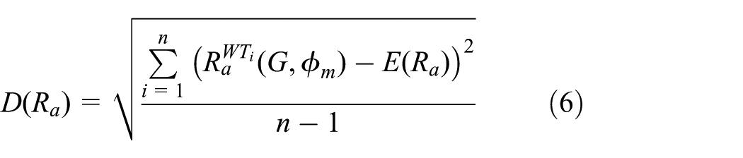
Then, we can obtain the average connectivity for all the MRs/MGs

The overall network connection fairness of MRs/MGs can be evaluated by the variance of their connectivity as follows

With formulations (5), (6), (8), and (9), we can evaluate the comprehensive robustness performance of the mesh network as

Here,
Network load-balancing performance
It is also very important to achieve better load-balancing performance when placing the MRs/MGs. An MR/MG may fail to work because of too heavy network traffic load and congestion, which will further cause a wide range of network connection failures. In order to improve the network stability and robustness, we propose to evaluate the overall network load-balancing performance with the function presented in formula (11)

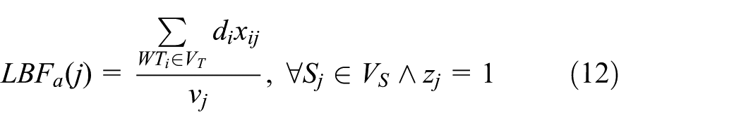

Here, the values of
Deployment cost
Under the premise of enhancing the robustness of the network, the deployment cost is also an important factor for planning and constructing the mesh network. Given the above parameters and variables, the optimization objective of deployment cost can be modeled as follows
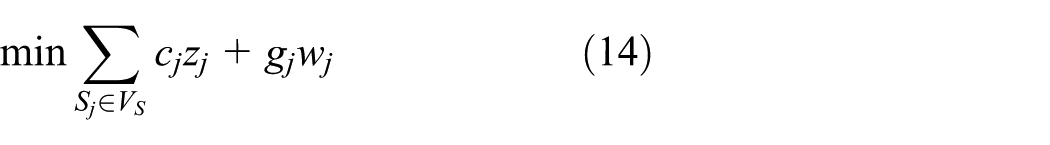
This objective accounts for the total cost of the placement of MRs and MGs with the installation cost cj and (cj + gi), respectively.
The problem
Our problem is to deploy the MRs/MGs by selecting the CLs to form a robust mesh network, where each WT is connected with two-coverage and each MR or MG is connected with two-connectivity, with the objectives of maximizing the network robustness performance as well as minimizing the load imbalance and the deployment cost. Given the above three optimization objectives presented in section “Objective function,” our multi-objective robustness optimization model for the deployment of MRs/MGs is therefore formulated as follows


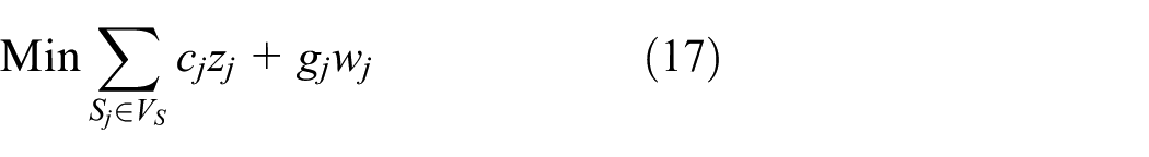
s.t.
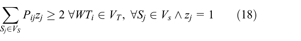


Formulas (15)–(17) represent three objective functions. Constraint (18) guarantees the two-coverage of all WTs, and Pij = 1 imposes that a wireless terminal WTi can be connected by an MR/MG deployed at Sj with one-hop or multi-hop network links among WTs. Constraint (19) assures that a deployed MR/MG should be at least connected with two other MRs/MGs, which guarantees the two-connectivity for each MR/MG.
Constraint (20) imposes that each WTi should be assigned to a deployed MR/MG. Constraint (21) imposes that all the WTs’ traffic serviced by an MR/MG does not exceed the capacity of the wireless link used for the access. Constraint (22) defines the traffic balance of an MR/MG deployed at Sj, the term
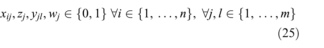
Constraint (23) defines that the total traffic on the link between MRs/MGs deployed at Sj and Sl does not exceed the capacity ujl of this link itself. Constraint (24) forces the flow between the device at Sj and the wired network to zero if the device at Sj is not an MG, and TF is the traffic capacity of the link between the MG and the wired network. Constraint (25) restricts the decision variables to take binary values.
Optimization algorithm for robust collaborative networking problem
The robust collaborative networking problem presented in section “The problem” is a multi-objective optimization problem with multiple constraints, which has a set of Pareto optimal solutions. Each solution represents a different optimal trade-off between multiple objectives and is said to be “non-dominated,” and the set of all the Pareto optimal solutions is the Pareto front. 14 In this article, we propose a multi-objective optimization method to solve our robust collaborative networking problem based on PSO algorithm.
Binary PSO
PSO 15 is an adaptive evolutionary computing technique proposed by Kennedy and Eberhart. PSO is a population-based optimization tool and inspired by the social behavior of natural individuals. It searches the optimal solution/particle for a difficult optimization problem through the collaboration between the individuals. Assume that the size of swarm is P, the coordinate position of each particle pi (i = 1∼N) at time t is denoted as xi(t) = (xi1(t), xi2(t), …, xiD(t)), and the particle velocity is defined as the moving distance at each search-iteration, which is represented by vi(t) = (vi1(t), vi2(t), …, viD(t)). At each search-iteration, the current position and velocity of each particle are updated by two best values: (1) pbest, individual best position that has achieved so far, and (2) gbest, another best value representing the global best position among all particles in the swarm. Then the particle pi updates its dth dimensional velocity and position according to the following formula

Here, w is the inertia weight factor which represents the impact of previous values of particle velocities on its current ones. A larger inertia weight factor is suitable for global exploration and a smaller inertia factor is suitable for fine-tuning in the current search area. Parameters c1 and c2 are positive constants called acceleration coefficients; in general, c1 = c2 = 2. Parameters r1 and r2 are two random variables with range [0, 1].
Currently, PSO algorithm has got various successful applications in many continuous optimization problems, but is seldom applied at dispersed land. In order to solve discrete combinatorial optimization problem, binary PSO (BPSO; a discrete binary version of PSO) 15 has been designed by Kennedy and Eberhart subsequently.
In BPSO, the positions of the particles in the binary model are indicated by two values, 1 and 0. Therefore, new definitions for velocity must be presented, and the velocity of each particle states the probability of being its position equal to 1. BPSO algorithm exploits a sigmoid transformation to the velocity component in order to force the velocities into the value between 0 and 1. The position of each particle is updated by the following rules


Here, rand is a random number in the interval [0, 1].
Improved binary MOPSO based on self-adaptive evolutionary learning
In order to solve the multi-objective optimization problem with multiple constraints, based on the original MOPSO algorithm, we have exploited an improved and more efficient binary MOPSO algorithm with a self-adaptive evolutionary learning method. This proposed algorithm modifies the evolutionary learning formula of the MOPSO algorithm according to the violation degree of the particles that are not meeting the constraints. Meanwhile, we introduce a dynamic maintenance strategy for Pareto optimal particles (solutions) based on crowding distance. With these methods, the Pareto front consisting of all the Pareto optimal particles obtained by the proposed algorithm has gained better performance of convergence, distribution, and diversity.
Self-adaptive evolutionary learning method
First, without loss of generality, all the constraints in our optimization problem can be expressed as equality and inequality constraints as follows

Here,

Then, according to the value of constraint violation level, the particles can be divided into two categories: feasible and unfeasible. For the feasible particles, they can update their velocities and positions in accordance with the standard BPSO algorithm. However, for the unfeasible particles, they should update their velocities and positions according to their constraint violation levels, and the values of their constraint violation levels are normalized as follows

The adaptive evolutionary learning formula for unfeasible particles can be described as follows
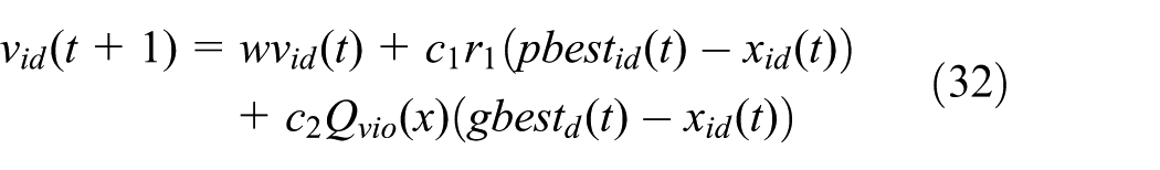
By analyzing formula (32), the unfeasible particles are able to achieve their evolutionary learning with their constraint violation levels. For those particles near the constraint boundary region, the values Qvio(x) of constraint violation levels are close to 0, which imposes that the global optimal solution becomes less attractive to the particles. The particles are able to approach the global optimal solution with smaller steps and explore the constraint boundary region more carefully. In addition, for those particles with large constraint violation levels,
A dynamic strategy for maintaining the distribution of the Pareto front based on the crowding distance
Because it will increase the complexity of the algorithm for maintaining all the Pareto optimal particles, it is quite necessary to optimize and confine the total size of the Pareto optimal particles. Meanwhile, a uniform distribution of the Pareto front can provide candidate particles with better diversity for the decision-makers. Crowding distance is commonly used to measure the aggregation density of individuals and can be used for the maintenance of the distribution of the Pareto front. Crowding distance can be computed as

Here, Ii is the crowding distance of the ith optimal solution, and M is the total number of optimization objective functions. Before computing the crowding distance, all the Pareto optimal particles are ranked according to ascending order in a dimension of multiple optimization objectives, and Ui,k is the value of the kth objective function of the ith optimal particle.
When the number of Pareto optimal particles exceeds a certain threshold, it is necessary to remove some redundant particles. The traditional methods for maintaining the distribution of the Pareto front based on crowding distance are likely to cut out too many particles in dense regions, which may result in missing some valuable Pareto optimal particles. Therefore, in order to avoid to erroneously delete the Pareto optimal particles, in our study, we put forward an improved dynamic method for maintaining the size and distribution of the Pareto front based on crowding distance. The specific maintenance process is introduced as follows:
Step 1. Calculate the crowding distance of all the Pareto optimal particles, and then sort all the Pareto optimal particles according to their respective values of crowding distance in descending order.
Step 2. According to the ranking results in step 1, the optimal solution with the smallest crowding distance will be removed in order to maintain the size and distribution of the Pareto front. If there are two Pareto optimal particles with the same crowding distance, one of them will be removed randomly.
Step 3. Judge whether the number of residual Pareto optimal particles exceeds a certain threshold, and if it exceeds, the maintenance process will switch to step 1; otherwise, the maintenance process will be finished.
Obtain the Pareto front of robust collaborative mesh networking problem with improved binary MOPSO algorithm.
With the improved binary MOPSO algorithm based on self-adaptive evolutionary learning, we are able to obtain the Pareto front of the multi-objective optimization model for robust collaborative mesh networking presented in section “The problem.” The pseudo code of our algorithm is shown in Algorithm 1. The outputs of this algorithm are POS_fitness and POS_position, which are the matrices of fitness (the value of network robustness and load-balancing performance evaluation metric presented in formulas (10) and (11)) and positions for the Pareto optimal particles in the Pareto front, respectively. GT and GS are the network graphs of the WTs and candidate deployment locations for MRs and MGs, respectively.

In addition, pi(t) = (pi1(t), pi2(t), …, pid(t), …, piD(t)) is the position of particle pi at the tth iteration, and it also represents an MR/MG deployment scheme. When an MR/MG is deployed at the dth CL, pid(t) will be set to 1, otherwise it will be set to 0. Here, D is the dimension of position and velocity of a particle, and its value is twice as much as the number of CLs for MRs/MGs. Meanwhile, (pi1(t), pi2(t), …, piD/2(t)) and (pi(D/2 + 1)(t), …, piD(t)) represent the deployment schemes of MRs and MGs, respectively. vi(t) = (vi1(t), vi2(t), …, vid(t), …, viD(t)) is the velocity of particle pi at the tth iteration. pbesti(t) is the individual best position of particle pi so far during t iterations, and gbest(t) is the global best position so far during t iterations.
In Algorithm 1, the sub-function initialize( ) randomly generates the positions and velocities of the particles with the input parameters including GS, Num_MR, and Num_MG. CheckifValid( ) checks whether a particle satisfies the constraints defined by formulas (18)–(24). The deployment schemes {zj} and {wj} of MRs and MGs can be directly obtained with the position of a particle pi(t). Based on the network graphs GT and GS, we can quickly calculate the results of the left or right parts in formulas (18)–(24). If any constraint is not satisfied, the particle is judged to be an unfeasible particle.
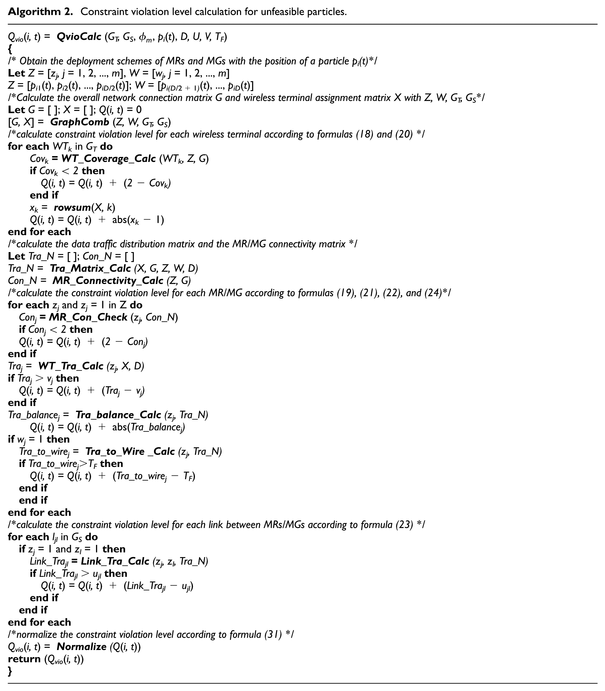
The sub-function QvioCalc( ) calculates the constraint violation level for each unfeasible particle pi(t), and the pseudo codes are presented in Algorithm 2. The sub-function FitnessCalc( ) obtains network robustness and load-balancing performance for each feasible particle pi(t), and the pseudo codes of this sub-function are presented in Algorithm 3.

Due to space limitation, the detailed pseudo codes of other sub-functions are not presented here. The sub-function ParetoFrontCalc( ) is responsible for calculating the Pareto optimal particles and removing some redundant particles according to the crowding distance defined by formula (33). The sub-function BestPositionInit( ) initializes the individual and global best position with the initial set of particles. BestPositionRefresh( ) refreshes the individual and global best position with the Pareto optimal particles obtained in each iteration according to the following rules:
If the size of the Pareto front = 0, the particle with the smallest constraint violation level will be selected as the global best position gbest(t).
If the size of the Pareto front > 0, the particle with the largest crowding distance in the Pareto front will be selected as the global best position gbest(t).
If all the historical positions of pi are unfeasible, the position with the smallest constraint violation level will be selected as the individual best position pbesti(t).
If not, the historical position of pi closest to the Pareto front will be selected as pbesti(t).
The sub-function ParticleUpdate_1( ) updates the position and velocity of the particle which is feasible in the last iteration, and ParticleUpdate_2( ) is responsible for updating the particle which is unfeasible in the last iteration according to formula (32). The computational complexity of Algorithm 1 is O(M(N + L)2), where M is the total number of optimization objectives.
As shown in Algorithm 2, the output parameter Qvio is an N × K two-dimensional (2D) matrix which saves the constraint violation level of each particle pi(t) in every iteration. First, the function QvioCalc( ) obtains the deployment matrices Z and W of MRs and MGs with the position of a particle pi(t), and then it calculates the overall network connection matrix G and WT assignment matrix X with the sub-function GraphComb(). Second, with the sub-function WT_Coverage_Calc( ), we obtain the coverage degree Covk of WTk and then calculate the constraint violation level based on formulas (18) and (20). Third, this algorithm calculates the network traffic distribution matrix Tra_N with Tra_Matrix_Calc() and the network connectivity matrix Con_N of MRs/MGs with MR_Connectivity_Calc(). For each MR/MG deployed at Sj, its network connectivity Conj, total data traffic Traj from WTs, the traffic balance Tra_balancej, and the traffic to the wired network Tra_to_wirej are calculated, and then the constraint violation level is calculated according to formulas (19), (21), (22), and (24). Fourth, the data traffic Link_Trajl on each link ljl between different MRs/MGs is calculated with the sub-function Link_Tra_Calc( ), and the constraint violation level for each link is obtained with formula (23). Finally, the total constraint violation level is normalized according to formula (31).
As shown in Algorithm 3, according to the evaluation model presented in section “Objective function,” the function FitnessCalc( ) calculates the network robustness and load-balancing performance for each particle pi(t). The results are saved in both the 2D matrices: fitness_Robust_Matrix and fitness_LBF_Matrix. First, with the sub-function Graph_Diversity_Calc( ) which exploits the exhaustive search algorithm, we can obtain the matrix R of k-terminal diversity for the WTs. The network connectivity matrix C of MRs/MGs is calculated with the sub-function MR_Connectivity_Calc( ). Then, the overall network robust performance can be calculated with formula (10). Second, with the network traffic distribution matrix Tra_N obtained by Tra_Matrix_Calc( ), the values of the accessing load-balancing factor LBFa and transferring load-balancing factor LBFb are calculated with the sub-functions LBF_A_Calc( ) and LBF_B_Cal( ), respectively. Then, the overall load-balancing performance is obtained with formula (11).
Experiments and results
In this section, the performance of the proposed MOPSO method for solving the multi-objective robust collaborative mesh networking problem is evaluated by simulating the related models and algorithms with MATLAB.
Experiment scenario
The related parameter settings for the experiment scenario are described in Table 1.
The experimental parameter setting.
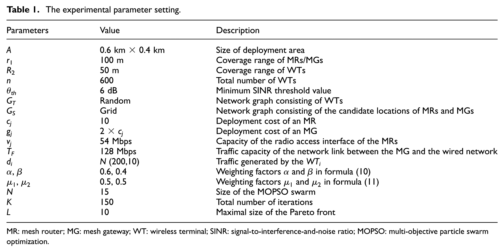
MR: mesh router; MG: mesh gateway; WT: wireless terminal; SINR: signal-to-interference-and-noise ratio; MOPSO: multi-objective particle swarm optimization.
As shown in Table 1 and Figure 2, the deployment area A of a factory is assumed to be a rectangle of 0.6 km × 0.4 km. The coverage range of MRs/MGs and WTs is 100 and 50 m, respectively. The total number of WTs (represented by red stars) is set to n = 600, and the WTs are randomly distributed in the region. We can then obtain the matrix of the connectivity parameters eij between WTs.
The deployment cost of an MR is cj = 10 for all the candidate locations, and the additional cost required to install an MG is gj = cj. The capacity of the radio access interface of all the MRs is vj = 54 Mbps, as well as the traffic capacity ujl between both MRs and MGs. The traffic capacity of the network link between the MG and the wired network TF = 128 Mbps. The traffic generated by the WTs di is assume to follow normal distribution with the parameters µ = 200 Kbps and
As shown in Figure 2, in order to obtain CLs VS = {S1, …, Sm} for MRs/MGs, for simplicity, we divide the deployment area into grid cells with the diagonal length equal to the communication range of MRs/MGs, and the CLs are assumed to be the grid intersections (represented by blue circles). Then, the number of CLs is set to 70, and this set of CLs is able to provide high redundant coverage of the deployment area, and then based on the proposed MOPSO algorithm, we search for the optimal subset with the best balance among multiple optimization objectives.
Analysis of experimental results
Pareto front of our multi-objective optimization problem
First, as shown in Figure 3, we simply investigate how the network performance (network robustness and load-balancing performance) change along with different numbers of deployed MRs/MGs with a fixed number of MGs. The number of MGs is assumed to be a fixed value

The Pareto front for deploying different numbers of MRs/MGs including seven MGs: (a) the Pareto front with 30 MR/MGs, (b) the Pareto front with 35 MR/MGs, (c) the Pareto front with 40 MR/MGs, and (d) comparison of different Pareto fronts.
In Figure 3, the X-axis and Y-axis, respectively, represent the network load-balancing and robustness performance of the Pareto optimal particles in the Pareto front, which are evaluated by formulas (10) and (11), respectively. It is worth noting that the network robustness performance is better with a higher value, as well as the load-balancing performance is better with a lower value. With the improved MOPSO algorithm of maintaining the distribution of the Pareto front based on the crowding distance, it is shown that the population size of particles in each Pareto front has been controlled. Meantime, as shown in Figure 3(d), with the comparison of the Pareto fronts for different numbers of MG/MGs, we can notice that the Pareto front has gained better performance of higher network robustness and better network load-balancing with the increasing number of MRs. Obviously, more MRs/MGs will improve network robustness performance and reduce average network traffic load; however, it also indicates that higher deployment cost is needed.
Furthermore, considering three optimization objectives (overall network robustness, load-balancing, and deployment cost), we measure the performance of our proposed method by exploring the Pareto front with different numbers of MRs/MGs including a fixed number of MGs = 7, as shown in Figure 4. We can notice that the particles in the three-dimensional (3D) Pareto front gather together with a clear divide line for different sections of the number of MRs/MGs (30–35, 36–40, 41–45, 46–50 with different markers and colors), which denotes that the number of MRs/MGs greatly affects the overall network performance. We also can find out that the scale of the 3D Pareto front is getting bigger because of more feasible deployment schemes. Meanwhile, the overall network robustness and load-balancing performance have been improved obviously along with the increasing number of MRs/MGs, which also means more deployment cost. With the 3D Pareto front, we are able to find out the minimal number of required MRs/MGs when given the thresholds of network robustness and load-balancing performance.
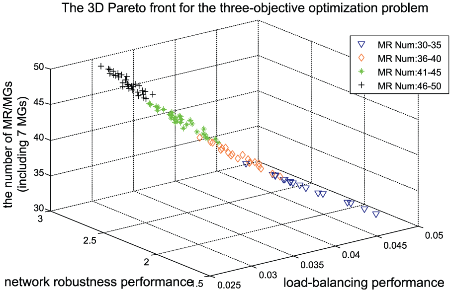
The 3D Pareto front for three optimization objectives with the improved MOPSO algorithm.
With the optimal particles in the 3D Pareto front, we then deeply investigate and analyze how network robustness performance and load-balancing performance change along with the deployed number of MRs/MGs, as shown in Figures 5 and 6. In Figure 5, the results show that the network robustness performance generally gets better along with the increasing number of MRs/MGs. However, when considering the average value of the network robustness performance of the optimal particles in the 3D Pareto front, we can notice that the gradient of the curve line of average value varies in different intervals of the number of MRs/MGs. Obviously, the network robustness performance increases fast when the number of MRs/MGs changes between 30 and 37, and then increases slowly when between 37 and 42, and then increases faster when between 42 and 50. This is because the network robustness performance is affected by the network interference, which is not expected to increase linearly with increasing node density. 16 In addition, as shown in Figure 6, the value of network load-balancing performance metric of the particles in the 3D Pareto front decreases approximately linearly along with the increasing number of MRs/MGs, which also means that it gets better network load-balancing.

The network robustness performance changes along with the total number of MRs/MGs (including seven MGs).

The network load-balancing performance changes along with the total number of MRs/MGs (including seven MGs).
Second, with a fixed number of MRs/MGs = 35 including different numbers of MGs (set to 4, 7, and 10, respectively), the Pareto front of network robustness and load-balancing performance has been explored by the proposed improved MOPSO algorithm, which is shown in Figure 7. Here, along with the increasing number of MGs, we can notice that the performance of the Pareto front has been improved a little, and the Pareto front moves in a certain direction with higher network robustness and better network load-balancing. This is because more MGs can balance the network traffic distribution and improve the network connection robustness between WTs and MGs. In addition, it is shown that the network performance has been improved with an increase in the number of MRs when compared with an increase in the number of MGs.

The Pareto front for deploying different numbers of MGs with 35 MRs/MGs: (a) the Pareto front with 4 MGs, (b) the Pareto front with 7 MGs, (c) the Pareto front with 10 MGs, and (d) comparison of different Pareto fronts.
Third, as shown in Figure 8, the Pareto front for network robustness and load-balancing performance has been evaluated with different numbers of WTs and a fixed number of MRs and MGs (set to 35 and 7, respectively). Along with the increasing number of WTs, we can notice that the value of network load-balancing performance metric of the particles in the Pareto front has increased significantly. Meanwhile, the average network robustness performance has increased not much along with more network paths among each WT and the set of MGs and better network connectivity, and this is because higher density of WTs brings more serious network interference and the network links are more likely to fall into failure.

The Pareto front for different numbers of WTs with 35 MRs/MGs (including seven MGs): (a) the Pareto front with 400 WTs, (b) the Pareto front with 600 WTs, (c) the Pareto front with 1000 WTs, and (d) comparison of different Pareto fronts.
Performance evaluation of the optimization ability of the improved MOPSO algorithm
In this section, with different numbers of MRs/MGs (35 and 40) including 7 MGs, we evaluate the performance of the improved MOPSO algorithm by comparing with the original MOPSO algorithm, which is shown in Figures 9 and 10 The experimental results showed that (1) the particles in the Pareto front of the original MOPSO algorithm have gathered together with higher density, and the distribution performance of the Pareto front is worse than the improved MOPSO algorithm because the original MOPSO algorithm is easy to fall into local optimum. (2) The Pareto front explored by the original MOPSO algorithm has worst performance on network robustness and load-balancing. These results are because of the fact that the local exploring capability in the constraint boundary region and global exploring capability have been enhanced with the improved MOPSO algorithm, which helps improve the performance on distribution and diversity of the Pareto front.

The Pareto front searched by the improved MOPSO and original MOPSO algorithm with 35 MRs/MGs (including seven MGs).

The Pareto front searched by the improved MOPSO and original MOPSO algorithm with 40 MRs/MGs (including seven MGs).
Deployment schemes
In this section, as an example, by selecting a particle with better balancing between overall network robustness and load-balancing performance in the Pareto front, we present a feasible deployment scheme obtained by the improved MOPSO algorithm with 35 MRs/MGs including 7 MGs, which is shown in Figure 11. In this deployment scheme, two-connectivity for MRs and two-coverage for WTs are guaranteed. We can also notice that most MRs (represented by blue circles) are distributed in the area with higher density of WTs, and the MGs (represented by green diamond) are evenly distributed in the deployment area to enhance the network load-balancing performance.
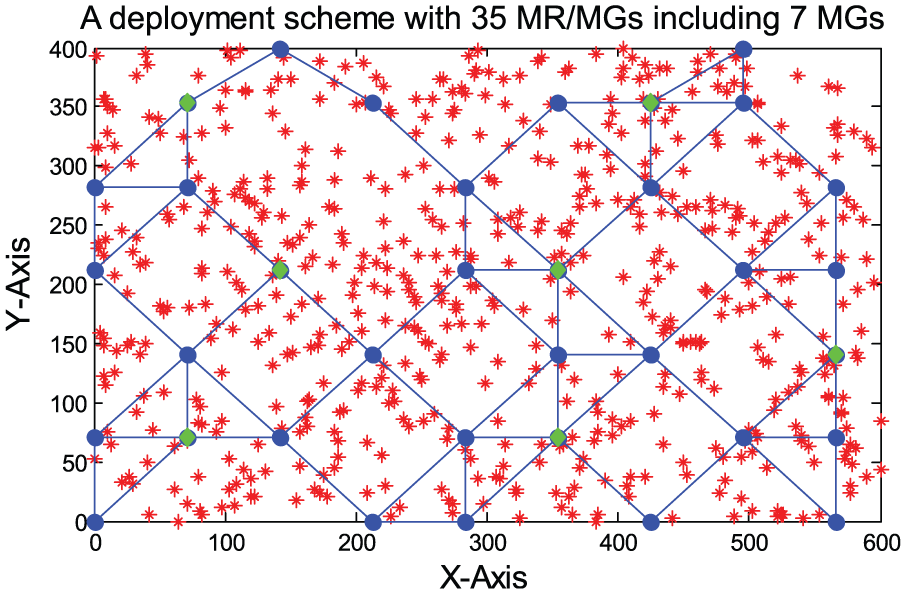
A deployment scheme with 35 MRs/MGs (including seven MGs).
Related works
In this section, we will investigate the related works of planning and constructing a high-performance WMN. In recent years, many efforts have been made to study the placement problem of MR and gateway nodes in WMNs in order to optimize some performance measures of WMNs. These previous works can generally be classified into two categories. The first category focuses on tailoring the placement problem by introducing different optimization objectives for fulfilling kinds of practical requirements. Usually, the optimization objectives include minimizing the overall deployment cost of MRs and gateways,15,17 maximizing the overall network throughput, 18 improving load-balancing performance, 19 ensuring full coverage of WTs, 20 and so on.
Amaldi et al. 12 have proposed a typical optimization model and method where the objective is to minimize the network installation cost while providing full coverage to wireless mesh clients (MCs). Benyamina et al. 15 proposed a multi-objective optimization model where network deployment cost and channel interference are simultaneously minimized while ensuring full coverage for WTs. They also proposed an algorithm for constructing reliable WMN infrastructure that resists the failure of a single mesh node and ensures full coverage to all MCs. 17 For dense WMNs, Avakul et al. 18 proposed to use graphs to represent multi-tier WMN and then determine the set of MRs that can be safely removed from the network without severing any connectivity of the network. Moreover, Sakamoto et al. 19 comprehensively evaluated the overall network connectivity using their proposed MR placement algorithm–WMN–simulated annealing (SA) under different distributions of MCs.
Taking into account the link vulnerability in wireless networks, Egeland and Engelstad 20 provided a method to forecast how the introduction of redundant nodes increases the reliability and availability of such networks. Kandah et al. 21 constructed an interference-aware network topology for the nodes and set up a pair of link–disjoint paths for each request with fault-tolerant capability. To provide network access and connectivity for wireless nodes, Shan et al. 22 proposed a novel reinforced backbone network (RBN) deployment method considering the practical limitation in the number of available backbone nodes and enforcing backbone network connectivity. Olascuaga-Cabrera et al. 23 presented a cluster-based self-organizing strategy for building a robust network backbone among the wireless devices, namely sensors, PDA, and cell phones. Moreover, a recent work by Lin et al. 24 investigated a more realistic router node placement (RNP) problem with a service priority constraint, and a novel SA approach with momentum terms was proposed to improve the efficiency and accuracy of finding the optimal solutions.
Furthermore, some previous works focus on providing robust network connectivity for mobile devices. Dong and Bejerano 25 studied the problem of building robust topologies (i.e. two-node/edge-connected) for nomadic WMNs, where the degree of any node does not exceed its number of available directional mesh radios. Shen et al. 26 proposed an autonomous mobile mesh network which is capable of organizing the mobile MCs into a suitable network topology to ensure good connectivity for both intra- and intergroup communications.
With kinds of multi-objective optimization models, the second category mainly focuses on designing effective multi-objective optimization algorithm, including SA,19,24 genetic algorithm (GA),27,28 PSO,15,17 and so on. Lin et al. 27 applied GAs for multiradio WMN planning, and they have demonstrated that GA is quite promising for solving complex discrete models involved in multichannel multiradio (MCMR) WMNs. Xhafa et al. 28 showed that GA is very efficient at computing placement of MR nodes and almost always achieves to establish connectivity of all MR nodes. Benyamina et al. 29 exploited a multi-objective optimization algorithm—MOPSO—to solve the problem where the total deployment cost and network throughput are to be optimized while guaranteeing full coverage to all MCs. Barolli et al. 30 presented some multi-objective optimization problems in WMNs and different heuristic methods such as local search, GAs, and Tabu search for solving them near-optimally.
As stated above, although there are many previous works for planning and constructing a mesh network with kinds of optimization objectives, the research work on planning high-performance WMNs in the industrial environment is currently relatively rare. Furthermore, planning WMNs in ICPSs has more stringent requirement on network robustness, reliability, and scalability while facing more prominent and severe environmental constraints including worst reliability of network nodes, more vulnerable network links, and more unbalanced distribution of network traffic. Specifically, the existing studies of deploying WMNs are challenged when applied in the industrial environment for the following limitations:
Most existing studies only implement one-coverage of WTs; however, an MR/MG would be more prone to be failed because of worst working condition and then the WTs are isolated, so it is necessary to implement k-coverage of WTs.
In most existing studies, a WT is only considered to be connected with MRs/MGs with a single hop, which greatly limits the coverage of MRs/MGs and increases the deployment cost too much. Therefore, in the industrial environment, the WTs should be equipped with the capability of multi-hop data transferring, which is very helpful for increasing the network connectivity and the coverage of MRs/MGs, and then decreasing the overall deployment cost.
Although some existing studies have considered the wireless link vulnerability, however, to some extent their link failure models are simple and the network inter-node interference is rarely concerned. In order to evaluate the network robustness performance more practically, it is necessary to exploit a more practical link failure model.
Therefore, with the above shortcomings of the existing studies, it is very necessary to develop high-performance collaborative mesh networking method for large-scale distributed WTs in ICPSs.
Conclusion and future works
In this article, for the network deployment optimization in ICPSs, we have proposed a robust collaborative mesh networking method with large-scale distributed wireless heterogeneous terminals. Due to the high requirement of network robustness and reliability, we introduced appropriate redundancy for the deployment of MRs and MGs to guarantee two-connectivity of MRs and two-coverage of WTs and also proposed related evaluation metrics for network robustness performance. Considering three pivotal optimization objectives including network robustness, load-balancing, and deployment cost, our robust collaborative mesh network problem is mathematically formulated as a multi-objective optimization problem with multiple constraints, and an improved binary MOPSO algorithm is proposed to solve this problem. The experimental results showed that the algorithm is able to obtain the Pareto front with better distribution and diversity and provide some alternative and effective network deployment options for decision-makers. Based on the studies in this article, an improved network deployment method with more random CLs of MRs and more dynamic and mobile WTs will be studied in our future work.
Footnotes
Academic Editor: Wei Yu
Declaration of conflicting interests
The author(s) declared no potential conflicts of interest with respect to the research, authorship, and/or publication of this article.
Funding
The author(s) disclosed receipt of the following financial support for the research, authorship, and/or publication of this article: This work was supported by the following funds in China, including the National Natural Science Foundation of China (61502110, 61672170), Projects of Science and Technology Plan of Guangdong Province (2017A010101017, 2013B010134011, 2015B010104005, and 2016B090918045), and the Key Program of NSFC-Guangdong Joint Funds (U1201251).