Distributed simultaneous localization and mapping for mobile robot networks via hybrid dynamic belief propagation

Abstract

This article proposes a hybrid dynamic belief propagation for simultaneous localization and mapping in the mobile robot network. The positions of landmarks and the poses of moving robots at each time slot are estimated simultaneously in an online and distributed manner, by fusing the odometry data of each robot and the measurements of robot–robot or robot–landmark relative distance and angle. The joint belief state of all robots and landmarks is encoded by a factor graph and the marginal posterior probability distribution of each variable is inferred by belief propagation. We show how to calculate, broadcast, and update messages between neighboring nodes in the factor graph. Specifically, we combine parametric and nonparametric techniques to tackle the problem arisen from non-Gaussian distributions and nonlinear models. Simulation and experimental results on publicly available dataset show the validity of our algorithm.

Introduction

There has been a significant interest in the mobile robot network composed of mobile robots that cooperate with each other due to its broad range of applications, such as target tracking, ¹ advanced manufacturing, ² disaster rescue, ³ and environment monitoring. ⁴ And one of the most critical steps about this technology is the simultaneous localization and mapping (SLAM) in an unknown environment. A solution to SLAM problem is beneficial to some special applications where precise environment information is not offered, for example, planetary exploration ⁵ and aerial vehicles. ⁶

We assume that some static landmarks are distributed randomly in a region, whose positions are unknown to us, and some mobile robots are freely moving around the area and having abilities of observation, storage, communication, and calculation. As robot nodes move, some relative measurements between a robot node and another robot or landmark are obtained. Our algorithm will make the most of these data to estimate the positions of landmarks and robots, poses of robots at all times. In the end, we utilize publicly available real dataset ⁷ to verify our method, whose founders also make some experiments^8–10 about decentralized solutions to SLAM in sparsely communicating robot networks and achieve good results based on this dataset which is thought suitable for our condition.

Recently, cooperative localization and mapping of multiple mobile robots arose many research interests. Considering the mode of resource allocation and algorithm implementation, the solutions are usually divided into centralized method and distributed method. The centralized localization algorithm can utilize observed data of the whole network to construct and update one common global map, which often gains high positioning accuracy at the expense of the computation and communication burden of central fusion node. For example, Wang et al. ¹¹ set a central entity independent of multi-robot system to collect local environmental maps from all robots, and then based on multi-source information used extended information filter to perform the global map update; while Choi and Lee ¹² carried out a master–slave structure, that is, selected the well-equipped master robot in the system as mobile center server grasping, processing, and transmitting the localization and mapping information; made other slave robots with comparatively simpler sensors perform only their localization tasks through unscented Kalman filter (UKF); and used mapping information received from the master robot to update information on slave robots. It is, however, inescapable that this kind of method is difficult to deal with the cases of the sparse communication connectivity, robot faults, and center node failure.

In contrast, the distributed estimation method has become an active field of wireless sensor networks (WSN), gradually replacing the centralized one. Distributed localization algorithms can accomplish local information processing and positioning with the aid of some near robots and then pass messages between nodes, whose computation burden is lower but positioning accuracy is comparable with centralized ones. In this branch, some detailed-oriented attention is being paid to communication constraints,^13–15 heterogeneity, ¹⁶ data association, ¹⁷ and so on.

Relatively, early and essential distributed SLAM algorithms are in state-space and particle filter (PF) form, which may be broad enough to contain Kalman filter (KF), extended Kalman filter (EKF), UKF, Rao-Blackwellized PF, PF, and so on. A distributed PF for implementing visual SLAM was proposed earlier by Won et al.,^18,19 which showed that the distributed SLAM system has a similar estimation performance and requires only one-fifth of the computation time compared with centralized PF; to tackle the limitation of particle impoverishment in generic PF, Pei et al. ²⁰ used improved PF to estimate the state vector of distributed SLAM, wherein adaptive values replaced a set of constants in the computational process of importance function used to calculate the probability of the particles in local filters, and two factors, the precision of the local filter and the number of effective particles, were mixed to calculate the weights of the local filters; nonetheless, PF has its drawbacks owing to its complexity as well as higher computational cost. Carlone et al. ²¹ extended Rao-Blackwellized PF application range from single-robot SLAM to multi-robot SLAM, and fused prioceptive and exteroceptive information from every robot to jointly estimate posterior of robots, but this needed completing a more complex reference frame transformation in the process of information fusion. Additionally, one significant challenge faced by these filtering techniques is minimizing the communication load between robots to avoid redundant data transmit and information double-counting.

The applications of factor graph model in such problems are also worth learning from. On one hand, a factor graph represents the multi-agent system mathematically and defines a nonlinear optimization problem that minimizes the error between the generative measurement and the actual measurement in the graph-based SLAM, whose factors plot measurement information, such as an observation of a landmark, odometry between poses, or prior information on a pose. For a typical graph-based SLAM system, the part of front-end complete the construction of the graph or data association, and a back-end puts emphasis on optimization by unknown graphs rather than direct processing of observation data. Cunningham et al.^22,23 developed decentralized data fusion-smoothing and mapping (DDF-SAM) focusing on the back-end, an extended SAM approach to implement DDF in the multi-robot distributed SLAM system, which consisted of single-robot local optimization module, communication module, and neighborhood graph optimizer module; with regard to specific techniques, it introduced constrained factor graphs used to represent the transforms between local and neighborhood frames of reference and Gaussian elimination, in which robots exchanged Gaussian marginals through separators; however, the marginals among robots were so crowded that communication cost was quadratic in the number of separators (i.e. variables observed by multiple robots), and Gaussian elimination was performed by a linearized version, which required to ensure consistent linearization across robots. In Casafranca et al., ²⁴ a solution based on minimizing the L₁ norm cost function was proposed as a back-end to the pose graph sub-problem, which had the primal-dual optimization formulation used to address nonlinear and non-differentiable L₁ function. The effort of Gulati et al. ²⁵ was mainly adding a kind of factors “topology,” that is, inter-vehicle distance, as constraints to the building of factor graph, for the sake of some challenges of bandwidth, data association uncertainties, coordinate transformation, and scalability in solutions to vehicle infrastructure cooperative localization. On the other hand, the factor graph model can be exploited to perform Bayesian inference algorithms recursively calculating the marginal distribution of each variable. Caceres et al. ²⁶ proposed H-SPAWN, a fully distributed cooperative positioning algorithm based on the sum–product algorithm over a factor graph, where a parametric message representation was introduced to reduce communication overhead; howbeit, since global navigation satellite system (GNSS) information can be acquired by terrestrial agents in this network, the nature of this problem is only mobile agents cooperative self-localization at each time slot, which is simpler than ours. In Wu et al., ²⁷ distributed Bayesian cooperative localization was solved via Gaussian message passing on factor graph, but nonlinearity between the positions and range measurements made the optimization problem complex and multivariate; therefore, the linearization on the Euclidean norm in the range measurement is employed, which ensured that closed-form expression can be obtained to represent the messages on factor. To further improve the closed-form Gaussian representation solutions to nonlinear observation model, the Taylor expansion was used to approximate the nonlinear terms in message updating, while a broadcast message scheme approximating the exact message passing was utilized to reduce the traffic burden in Li et al. ²⁸ But what cannot be ignored was that above studies^27,28 did not give an even generalized motion model, namely, the former offered a simple linear state-space model and the later did not mention it; and what was more, they required anchors whether or not accurate although the placement of anchor nodes was normally seen, for example Wymeersch et al. ²⁹ SPAWN, a cooperative localization method based on the sum–product algorithm and factor graph, was proposed in Wymeersch et al. ²⁹ and applied to ultra-wide bandwidth wireless networks; however, it distinguished between agents with priori unknown states and anchors with known states at all times, both of which may be mobile, and became extremely difficult in directly computing messages. On the whole, some message passing algorithms over factor graphs can be responsive to distributed cooperative localization problems; going a step further, we could consider to design an inference algorithm based on factor graph model to cope with the SLAM problem, which is a relatively less practice to the best of our knowledge.

In this article, we propose a distributed method based on belief propagation (BP) ³⁰ over a factor graph model for mobile multi-robot cooperative localization and mapping (MR.CLAM). The main contributions of our work are described as follows:

1. We translate the SLAM problem of mobile robot networks into the recursive calculation of the marginal posterior distribution of each random variable corresponding to every robot or landmark, which is based on all observations rooted in physical motion and observation models.

2. We encode the joint belief state of all objects (i.e. robots and landmarks) in the whole mobile robot network into a factor graph.

3. We propose a distributed inference algorithm, named hybrid dynamic BP, based on the sum–product algorithm over the previously constructed factor graph, which guarantees local message exchange between neighboring nodes, while do not need anchors and a central processing node in the entire system.

4. We employ a hybrid parametric and nonparametric information fusion technique to flexibly deal with nonlinear models and non-Gaussian distributions extensively arising in practice. We use Gaussian distribution to approximate the belief state, and meanwhile adopt particle sampling to resolve complicated message distributions.

5. We define a message passing matrix to directly represent message passing rules for updating belief state during iteration. The elements of this matrix indicating relative observations between neighboring nodes are updated in each iteration.

6. We verify the effectiveness of our method by simulation and experimental results on real dataset.

The remainder of the article is organized as follows: we formulate the problem in section “Problem formulation,” present our hybrid dynamic BP in section “Inference algorithm,” and show the simulation and experimental results in section “Results.” Finally, conclusion and the future plan are given in section “Conclusion.”

Problem formulation

In this section, we formulate the SLAM problem of mobile robot networks in a probabilistic framework. We can concretely consider that a fleet of mobile robots, each of which is equipped with an odometer and a monocular camera, move in a region with some static landmarks whose positions are unknown. Figure 1 shows the real environment built by the founders of publicly available dataset; ⁷ from the overall perspective, Figure 1(a) displays the detection scene, where robots (with pedestals) and landmarks are appearing.

Figure 1.

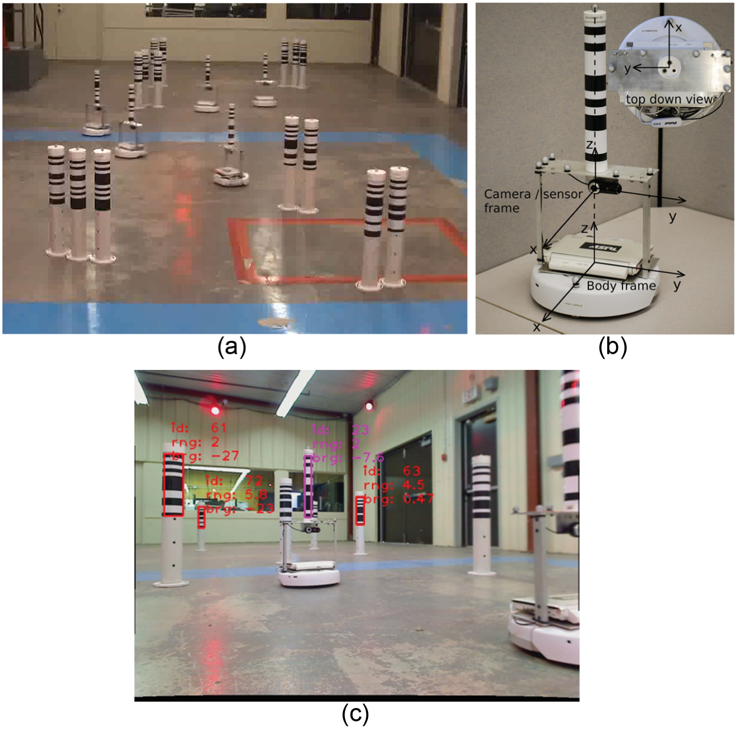
Real experimental environment in Leung et al.: ⁷ (a) macroscopic indoor view, (b) mobile robot body, and (c) observations from an undistorted image.

The odometer sensor outputs a robot’s odometry information $u$ , consisting of the robot’s forward velocity and angular velocity, where the covariance ${\Sigma }_{\mathrm{odo}}$ of process noise distribution is

$${\Sigma }_{odo}=\left[\begin{array}{cc}{\sigma }_v^2& 0\\ 0& {\sigma }_{\omega }^2\end{array}\right]$$

In a multi-robot system, let $I$ and $K$ represent the sets of unique identification indices of all robots and landmarks, respectively. At time $\tau$ , the state of the ith robot, $X_i^{\tau }=[x_i^{\tau },y_i^{\tau },{\theta }_i^{\tau }{]}^{\mathrm{T}}$ , contains its two-dimensional (2D) position in the global coordinate system and orientation determined by counterclockwise rotation from the x-axis of the global coordinate system to the robot body frame’s, and the state of the kth static landmark is its global position $L_k^{\tau }=[x_k^{\tau },y_k^{\tau }{]}^{\mathrm{T}}$ . According to the above settings and simplified moving mechanism of the wheeled equipment detailed in Figure 1(b), rather than considering their own complex structures, system characteristics, and force conditions of components, we treat every robot as a particle, and give general motion models for robots and landmarks

$$X_i^{\tau }=f(X_i^{\tau -1},u_i^{\tau },{\epsilon }_{odo}^{\tau })(\forall i\in I)$$

(1)

$$L_k^{\tau }=L_k^{\tau -1}(\forall k\in K)$$

(2)

where $f(·)$ is the state transition function (with the zero-mean Gaussian process noise ${\epsilon }_{\mathrm{odo}}=[{\epsilon }_x,{\epsilon }_y,{\epsilon }_{\theta }{]}^{\mathrm{T}}$ ) and defined as

$$\begin{array}{cc}\multicolumn{1}{c}{\left[\begin{array}{c}{x}_i^{\tau }\hfill \\ \multicolumn{1}{c}{y_i^{\tau }}\\ \multicolumn{1}{c}{{\theta }_i^{\tau }}\end{array}\right]}& =\left[\begin{array}{c}{x}_i^{\tau -1}+v_i^{\tau }\cos ({\theta }_i^{\tau -1}+w_i^{\tau }\Delta t)\Delta t\hfill \\ \multicolumn{1}{c}{y_i^{\tau -1}+v_i^{\tau }\sin ({\theta }_i^{\tau -1}+w_i^{\tau }\Delta t)\Delta t}\\ \multicolumn{1}{c}{{\theta }_i^{\tau -1}+w_i^{\tau }\Delta t}\end{array}\right]\hfill \\ \multicolumn{1}{c}{}& +\left[\begin{array}{c}{\epsilon }_x^{\tau }\hfill \\ \multicolumn{1}{c}{{\epsilon }_y^{\tau }}\\ \multicolumn{1}{c}{{\epsilon }_{\theta }^{\tau }}\end{array}\right]({\theta }_i\in [-\pi ,\pi ])\hfill \end{array}$$

(3)

where $\Delta t$ is sampling interval and generally a very small value, so we can utilize equation (3) to make the state of each robot evolve.

The camera serving as the main sensor captures undistorted images processed and used to offer relative range and bearing measurements (when another robot or landmark is in a robot’s field of view) at every time, as shown in Figure 1(c) from some robot’s perspective. A unique identification number of every robot or landmark is encoded as a barcode. During measurement data production, the camera on each robot is conveniently placed to align with the robot body frame to obtain the parameters necessary to undistorted images on which a process that primarily relies on edge detection is used for detecting barcodes. Figure 1(c) shows the typical output of the barcode detection process. Range measurements are obtainable since the vertical focal length and the barcode height are known; bearing measurements correspond to the horizontal position of a barcode in an image; for a detailed treatment, the reader is referred to Leung et al. ⁷ And the conception of a robot’s field of view is illustrated in Figure 2(a), in generally, every robot has the measurement range limit and detection angle restraint, $d_{\mathrm{obs}}$ and ${\phi }_{\mathrm{obs}}\le \pi$ . Robots within field of view of each other are able to measure the relative position of the other side, but when there is one-way observation, only observer can make measurements to the other one. For example, in Figure 2(a), X₅ is within field of view of X₄ and vice versa, so they can make measurements toward each other, and we use the solid line to represent this kind of pairwise observation in Figure 2(b); besides, X₅ is also within field of view of X₃ but the inverse is not, so only X₅ produces measurements regarding X₃, and we use the dashed line to represent such one-way relationship in Figure 2(b). Note, however, that information exchanging and message passing in the subsequent inference process are bidirectional for both sides involving observation events whether they are under pairwise or one-way measurement.

Figure 2.

Observation information communication of the mobile robot network: (a) diagram of environment detection and (b) network topology corresponding to (a).

We use $N_i^{\tau }$ to denote the set of the ith robot’s neighbors at time $\tau$ , containing all robots and landmarks within its field of view. The observation model outlined is as follows

$$Z_{\mathrm{in}}^{\tau }=q(X_i^{\tau },N_{\mathrm{in}}^{\tau },{\epsilon }_{\mathrm{obs}}^{\tau })(N_{\mathrm{in}}^{\tau }\in N_i^{\tau })$$

(4)

where for timestep $\tau$ , $N_{\mathrm{in}}$ represents some neighbor n (a robot or landmark) of robot i, and the observation made by robot i between it and neighbor n consists of the relative range and angle $Z_{\mathrm{in}}=[d_{\mathrm{in}},{\phi }_{\mathrm{in}}{]}^{\mathrm{T}}$ ; $q(·)$ is the measurement function and externalized as

$$\begin{array}{cc}\multicolumn{1}{c}{\left[\begin{array}{c}{d}_{\mathrm{in}}\hfill \\ \multicolumn{1}{c}{{\phi }_{\mathrm{in}}}\end{array}\right]}& =\left[\begin{array}{c}\sqrt{{(x_i-x_n)}^2+{(y_i-y_n)}^2}\hfill \\ \multicolumn{1}{c}{\arctan \left(\frac{y_n-y_i}{x_n-x_i}\right)-{\theta }_i}\end{array}\right]\hfill \\ \multicolumn{1}{c}{}& +\left[\begin{array}{c}{\epsilon }_d\hfill \\ \multicolumn{1}{c}{{\epsilon }_{\phi }}\end{array}\right](d_{\mathrm{in}}\in (0,d_{\mathrm{obs}}],{\phi }_{\mathrm{in}}\in [-\frac{{\phi }_{\mathrm{obs}}}{2},\frac{{\phi }_{\mathrm{obs}}}{2}])\hfill \end{array}$$

(5)

here, ${\epsilon }_{\mathrm{obs}}=[{\epsilon }_d,{\epsilon }_{\phi }{]}^{\mathrm{T}}$ is additive zero-mean Gaussian measurement noise, whose covariance is

$${\Sigma }_{\mathrm{obs}}=\left[\begin{array}{c}{\sigma }_d^{2}0\hfill \\ \multicolumn{1}{c}{0{\sigma }_{\phi }^2}\end{array}\right]$$

wherein $d_{\mathrm{in}}$ means Euclidean distance between geometric centers of robot $i$ and its neighbor’s, and ${\phi }_{\mathrm{in}}$ indicates the relative angle determined by counterclockwise rotation from the x-axis of the robot $i$ body frame to the line of two involved objects’ centers. More intuitive understanding with relative measurements is got by Figure 3, where the red dotted arrow stands for the x-axis of the robot body frame.

Figure 3.

Relative measurements between neighboring objects in 2D global coordinate system: (a) relative measurements of robot–landmark and (b) relative measurements of robot–robot.

From timestep 1 to $\tau$ , we use random variable $L^{1:\tau }=\{L_k^{1:\tau }\}(\forall k\in K)$ to denote the set of all landmark static positions, and use random variable $X^{1:\tau }=\{X_i^{1:\tau }\}(\forall i\in I)$ to denote the set of all robot states. Similarly, let $U^{1:\tau }$ and $Z^{1:\tau }$ represent the sets of all available odometry information and camera measurements made by all robots, respectively. The joint belief state of all robots and landmarks conditioned on all observation is

$$b(X^{1:\tau },L^{1:\tau })=p(X^{1:\tau },L^{1:\tau }|Z^{1:\tau },U^{1:\tau })$$

(6)

To solve the SLAM problem, we need to recursively calculate the marginal posterior distribution of each random variable.

Before giving the solution, it is necessary to list several primary hypotheses in the context of this article, each of which is also declared in the corresponding formula derivation:

• Every object in the network is treated as a particle;

• Robot motion model possesses Markov property;

• Additive process noise and measurement noise mentioned above follow zero-mean Gaussian distribution;

• Objects are independent of each other;

• The belief state of every object at each timestep can be approximated as Gaussian distribution.

Inference algorithm

In this section, we present our hybrid dynamic BP algorithm for calculating the marginal distributions. First in section “Graphical model,” we factorize the joint posterior distribution and represent it by a factor graph. Then, we specify eight types of messages in section “Message calculation.” Specially, we utilize both parametric and nonparametric representations to deal with complex probability distributions. We show the belief calculation in section “Belief calculation” and supplement some message passing particulars in section “Message passing schedule.”

Graphical model

On the premise of the Markov property of motion model, the joint posterior probability (6) can be expanded as

$$\begin{array}{cc}\multicolumn{1}{c}{b(X^{1:\tau },L^{1:\tau })=}& p(X^{\tau },L^{\tau }|X^{\tau -1},L^{\tau -1},Z^{\tau },U^{\tau })\cdots \hfill \\ \multicolumn{1}{c}{}& p(X^1,L^1|X^0,L^0,Z^1,U^1)b(X^0,L^0)\hfill \end{array}$$

(7)

where $b(X^0,L^0)$ represents initial states of all robots and landmark. For timestep $\tau$ , according to Bayesian theory and the independence between robot movements, we can factorize $b(X^{\tau },L^{\tau })$ as

$$\begin{array}{c}b(X^{\tau },L^{\tau })\stackrel{\Delta }{=}p(X^{\tau },L^{\tau }|Z^{1:\tau },U^{1:\tau })\hfill \\ =p(X^{\tau },L^{\tau }|X^{\tau -1},L^{\tau -1},Z^{\tau },U^{\tau })p(X^{\tau -1},L^{\tau -1}|Z^{1:\tau -1},U^{1:\tau -1})\hfill \\ \propto p(Z^{\tau }|X^{\tau },L^{\tau })p(X^{\tau },L^{\tau }|X^{\tau -1},L^{\tau -1},U^{\tau })b(X^{\tau -1},L^{\tau -1})\hfill \\ =\underset{i=1}{\overset{I}{\Pi }}\left[\underset{L_k^{\tau }\in N_i^{\tau }}{\Pi }p(Z_{\mathrm{ik}}^{\tau }|X_i^{\tau },L_k^{\tau })\underset{X_j^{\tau }\in N_i^{\tau }}{\Pi }p(Z_{\mathrm{ij}}^{\tau }|X_i^{\tau },X_j^{\tau })\right]\hfill \\ \underset{i=1}{\overset{I}{\Pi }}p(X_i^{\tau }|X_i^{\tau -1})\underset{k=1}{\overset{K}{\Pi }}p(L_k^{\tau }|L_k^{\tau -1})b(X^{\tau -1},L^{\tau -1})\hfill \end{array}$$

(8)

where we split the part about observations $p(Z^{\tau }|X^{\tau },L^{\tau })$ into robot–landmark measurements $p(Z_{\mathrm{ik}}^{\tau }|X_i^{\tau },L_k^{\tau })$ and robot–robot measurements $p(Z_{\mathrm{ij}}^{\tau }|X_i^{\tau },X_j^{\tau })$ , and similarly split the part about temporal state evolution $p(X^{\tau },L^{\tau }|X^{\tau -1},L^{\tau -1},U^{\tau })$ into robot’s $p(X_i^{\tau }|X_i^{\tau -1})$ and landmark’s $p(L_k^{\tau }|L_k^{\tau -1})$ . Hence, we define the following three kinds of factors:

• 1. Prediction factor

$$f_{X_i}(X_i^{\tau -1},X_i^{\tau })\stackrel{\Delta }{=}p(X_i^{\tau }|X_i^{\tau -1})$$

(9)

$$f_{L_k}(L_k^{\tau -1},L_k^{\tau })\stackrel{\Delta }{=}p(L_k^{\tau }|L_k^{\tau -1})$$

(10)

represent mobility.

• 2. Factor for robot–landmark observation

$$g_{\mathrm{ik}}(X_i^{\tau },L_k^{\tau })\stackrel{\Delta }{=}p(Z_{\mathrm{ik}}^{\tau }|X_i^{\tau },L_k^{\tau })$$

(11)

represents robot–landmark measurement likelihood given by the states of robot variable node $X_i$ and landmark variable node $L_k$ .

• 3. Factor for robot–robot observation

$$h_{\mathrm{ij}}(X_i^{\tau },X_j^{\tau })\stackrel{\Delta }{=}p(Z_{\mathrm{ij}}^{\tau },Z_{\mathrm{ji}}^{\tau }|X_i^{\tau },X_j^{\tau })$$

(12)

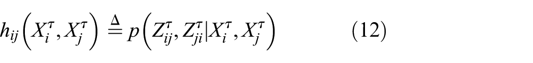
represents the peer-to-peer pairwise measurement likelihood given by the states of robot variable node $X_i$ and $X_j$ . Whereas there is also the one-way relationship, namely

$$h_{\mathrm{ij}}(X_i^{\tau },X_j^{\tau })\stackrel{\Delta }{=}p(Z_{\mathrm{ij}}^{\tau }|X_i^{\tau },X_j^{\tau })(X_j^{\tau }\in N_i^{\tau },X_i^{\tau }\notin N_j^{\tau })$$

(13)

or

$$h_{\mathrm{ij}}(X_i^{\tau },X_j^{\tau })\stackrel{\Delta }{=}p(Z_{\mathrm{ji}}^{\tau }|X_i^{\tau },X_j^{\tau })(X_i^{\tau }\in N_j^{\tau },X_j^{\tau }\notin N_i^{\tau })$$

(14)

And thus equation (8) can be represented by factors, and the belief state $b(X^{\tau },L^{\tau })$ is encoded by a factor graph shown in Figure 4, where a circle denotes a variable node for each mobile robot X_i, a triangle denotes a variable node for each landmark L_k, and a square denotes a factor node for each local function. On the basis of connection and message flows among nodes, some elementary observation information and statistical dependencies can be obtained from this graph, for example, robot X₄ notices landmark L₂ and L₃, and maybe see peer X₂ and X₃ at time $\tau$ . So far, we have translated the SLAM of mobile robot network into the inference problem on the graphical model.

Figure 4.

Factor graph model for inference in SLAM described in section “Problem formulation.”

Message calculation

We will use BP algorithm performed on above factor graph for distributed inference. Actually, BP is an iterative algorithm, and conducted by passing local messages between factor node and variable node to give the exact marginal probabilities for all the nodes in the graph, where the message is a function of the random variables. In this subsection, we will discuss how to compute the involved messages, which are listed in Table 1.

Table 1.

Summary of message types.

Message type	Notation	Parametric/nonparametric	Calculation formula
Prediction message of robot	$m_{f_{X_i}\to X_i}(X_i^{\tau })$	P	Formula (15)
Prediction message of landmark	$m_{f_{L_k}\to L_k}(L_k^{\tau })$	P	Formula (20)
Message from robot–landmark factor to landmark variable	$m_{g_{\mathrm{ik}}\to L_k}(L_k^{\tau })$	P	Formula (21)
Message from robot–landmark factor to robot variable	$m_{g_{\mathrm{ik}}\to X_i}(X_i^{\tau })$	P	Formula (25)
Message from robot–robot factor to robot variable	$m_{h_{\mathrm{ij}}\to X_i}(X_i^{\tau })$	P	Formula (29)
Message from landmark variable to robot–landmark factor	${m_{L_k\to }}_{g_{\mathrm{ik}}}(L_k^{\tau })$	NP	Formula (33)
Message from robot variable to robot–landmark factor	$m_{X_i\to g_{\mathrm{ik}}}(X_i^{\tau })$	NP	Formula (34)
Message from robot variable to robot–robot factor	$m_{X_i\to h_{\mathrm{ij}}}(X_i^{\tau })$	NP	Formula (35)

For each type of message, we first give the calculation formulas according to the simple update rule of sum–product algorithm. ³¹ Due to integrals and multiplications of higher-dimensional space existing in these formulas, we adopt parametric or hybrid strategies to simplify direct calculation. By this means, messages could be approximated by some widely known distributed families, which can be depicted as parameters. Here, we assume that the belief state is approximate to Gaussian distribution at every time:

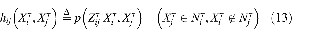
• 1. Prediction message of robot $m_{f_{X_i}\to X_i}(X_i^{\tau })$

For inter-slice prediction, each variable node representing the robot sends a time-forward message to its corresponding node in the next time

$$m_{f_{X_i}\to X_i}(X_i^{\tau })=\sum _{X_i^{\tau -1}}{f}_{X_i}(X_i^{\tau -1},X_i^{\tau })b(X_i^{\tau -1})$$

(15)

We use ${\mu }_{X_i^{\tau -1}}$ and ${\Sigma }_{X_i^{\tau -1}}$ to denote the mean and covariance of the distribution of $b(X_i^{\tau -1})$ , so there is

$$b\left(X_i^{\tau -1}\right)\approx N(X_i^{\tau -1};{\mu }_{X_i^{\tau -1}},{\Sigma }_{X_i^{\tau -1}})$$

(16)

further, $m_{f_{X_i}\to X_i}(X_i^{\tau })$ can be represented as

$$m_{f_{X_i}\to X_i}\left(X_i^{\tau }\right)\approx N(X_i^{\tau };{\mu }_{X_i^{\tau |\tau -1}},{\Sigma }_{X_i^{\tau |\tau -1}})$$

(17)

and parameters ${\mu }_{X_i^{\tau |\tau -1}}$ and ${\Sigma }_{X_i^{\tau |\tau -1}}$ of the distribution can be derived from robot motion models (1) and (3), respectively

$$\begin{array}{c}{\mu }_{X_i^{\tau |\tau -1}}=\left[\begin{array}{c}{\mu }_{x_i^{\tau |\tau -1}}\hfill \\ \multicolumn{1}{c}{{\mu }_{y_i^{\tau |\tau -1}}}\\ \multicolumn{1}{c}{{\mu }_{{\theta }_i^{\tau |\tau -1}}}\end{array}\right]=\left[\begin{array}{c}{\mu }_{x_i^{\tau -1}}+v_i^{\tau }\cos ({\mu }_{{\theta }_i^{\tau -1}}+w_i^{\tau }\Delta t)\Delta t\hfill \\ \multicolumn{1}{c}{{\mu }_{y_i^{\tau -1}}+v_i^{\tau }\sin ({\mu }_{{\theta }_i^{\tau -1}}+w_i^{\tau }\Delta t)\Delta t}\\ \multicolumn{1}{c}{{\mu }_{{\theta }_i^{\tau -1}}+w_i^{\tau }\Delta t}\end{array}\right]\hfill \\ ({\mu }_{{\theta }_i}\in [-\pi ,\pi ])\hfill \end{array}$$

(18)

$${\Sigma }_{X_i^{\tau |\tau -1}}={\Sigma }_{X_i^{\tau -1}}+F{\Sigma }_{\mathrm{odo}}{F}^{\mathrm{T}}$$

(19)

where transition matrix $F=\left[\begin{array}{c}10\hfill \\ \multicolumn{1}{c}{10}\\ \multicolumn{1}{c}{01}\end{array}\right]$ .

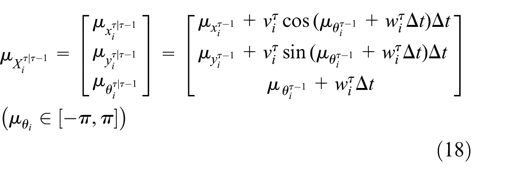
• 2. Prediction message of landmark $m_{f_{L_k}\to L_k}(L_k^{\tau })$

Similar to (1), this type of time-forward message about landmarks can be calculated by the motion model (2)

$$\begin{array}{c}{m}_{f_{L_k}\to L_k}\left(L_k^{\tau }\right)=\sum _{L_k^{\tau -1}}{f}_{L_k}(L_k^{\tau -1},L_k^{\tau })b\left(L_k^{\tau -1}\right)\hfill \\ \approx N(L_k^{\tau };{\mu }_{L_k^{\tau |\tau -1}},{\Sigma }_{L_k^{\tau |\tau -1}})\hfill \\ =N(L_k^{\tau -1};{\mu }_{L_k^{\tau -1}},{\Sigma }_{L_k^{\tau -1}})\hfill \end{array}$$

(20)

That is, ${\mu }_{L_k^{\tau |\tau -1}}={\mu }_{L_k^{\tau -1}}$ and ${\Sigma }_{L_k^{\tau |\tau -1}}={\Sigma }_{L_k^{\tau -1}}$

• 3. Message from robot–landmark factor to landmark variable $m_{g_{\mathrm{ik}}\to L_k}(L_k^{\tau })$

$$m_{g_{\mathrm{ik}}\to L_k}\left(L_k^{\tau }\right)=\sum _{X_i^{\tau }}{g}_{\mathrm{ik}}(X_i^{\tau },L_k^{\tau })m_{X_i\to g_{\mathrm{ik}}}\left(X_i^{\tau }\right)$$

(21)

$m_{X_i\to g_{\mathrm{ik}}}(X_i^{\tau })$ provides a pdf of $X_i^{\tau }$ , based on the available information collected from its all neighbors except $L_k$ , and we approximate this message as Gaussian distribution with current mean ${\mu }_{X_i^{\tau }}=[{\mu }_{x_i^{\tau }},{\mu }_{y_i^{\tau }},{\mu }_{{\theta }_i^{\tau }}{]}^{\mathrm{T}}$ and covariance ${\Sigma }_{X_i^{\tau }}$ ; thus, $m_{g_{\mathrm{ik}}\to L_k}(L_k^{\tau })$ is estimated by the distribution over $X_i^{\tau }$ and observation data $Z_{\mathrm{ik}}^{\tau }$

$$\begin{array}{c}{m}_{g_{\mathrm{ik}}\to L_k}(L_k^{\tau })\approx p(L_k^{\tau }|{\mu }_{X_i^{\tau }},d_{\mathrm{ik}}^{\tau },{\phi }_{\mathrm{ik}}^{\tau },{\Sigma }_{X_i^{\tau }},{\Sigma }_{\mathrm{obs}})\hfill \\ =N(L_k^{\tau };{\hat{\mu }}_{L_k^{\tau }},{\hat{\Sigma }}_{L_k^{\tau }})\hfill \end{array}$$

(22)

with estimated mean and covariance

$$\begin{array}{c}{\hat{\mu }}_{L_k^{\tau }}=\left[\begin{array}{c}{\hat{\mu }}_{x_k^{\tau }}\hfill \\ \multicolumn{1}{c}{{\hat{\mu }}_{y_k^{\tau }}}\end{array}\right]=\left[\begin{array}{c}{\mu }_{x_i^{\tau }}+d_{\mathrm{ik}}^{\tau }\cos ({\mu }_{{\theta }_i^{\tau }}+{\phi }_{\mathrm{ik}})\hfill \\ \multicolumn{1}{c}{{\mu }_{y_i^{\tau }}+d_{\mathrm{ik}}^{\tau }\sin ({\mu }_{{\theta }_i^{\tau }}+{\phi }_{\mathrm{ik}})}\end{array}\right]\hfill \\ ({\mu }_{{\theta }_i^{\tau }}\in [-\pi ,\pi ])\hfill \end{array}$$

(23)

$${\hat{\Sigma }}_{L_k^{\tau }}=H{\Sigma }_{X_i^{\tau }}{H}^{\mathrm{T}}+\Lambda {\Sigma }_{\mathrm{obs}}{\Lambda }^{\mathrm{T}}$$

(24)

where transition matrix $H=\left[\begin{array}{c}100\hfill \\ \multicolumn{1}{c}{010}\end{array}\right]$ and $\Lambda =\left[\begin{array}{c}10\hfill \\ \multicolumn{1}{c}{10}\end{array}\right]$ .

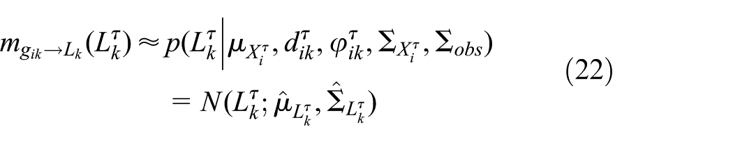
• 4. Message from robot–landmark factor to robot variable $m_{g_{\mathrm{ik}}\to X_i}(X_i^{\tau })$

$$m_{g_{\mathrm{ik}}\to X_i}\left(X_i^{\tau }\right)=\sum _{L_k^{\tau }}{g}_{\mathrm{ik}}(X_i^{\tau },L_k^{\tau })m_{L_k\to g_{\mathrm{ik}}}(L_k^{\tau })$$

(25)

The same principle can be easily adapted to assume that the current pdf of $L_k^{\tau }$ describes a Gaussian distribution, that is, $m_{L_k\to g_{\mathrm{ik}}}(L_k^{\tau })\approx N(L_k^{\tau };{\mu }_{L_k^{\tau }},{\Sigma }_{L_k^{\tau }})$ ; the resulting message is therefore expressed as

$$\begin{array}{c}{m}_{g_{\mathrm{ik}}\to X_i}\left(X_i^{\tau }\right)=p(X_i^{\tau }|L_k^{\tau },Z_{\mathrm{ik}}^{\tau })\hfill \\ =p(x_i^{\tau },y_i^{\tau }|{\mu }_{L_k^{\tau }},{\Sigma }_{L_k^{\tau }},d_{\mathrm{ik}}^{\tau },{\sigma }_d^2)\hfill \\ p({\theta }_i^{\tau }|x_i^{\tau },y_i^{\tau },{\mu }_{L_k^{\tau }},{\phi }_{\mathrm{ik}}^{\tau },{\sigma }_{\phi }^2)\hfill \\ =C(x_i^{\tau },y_i^{\tau };{\mu }_C,r_C,{\Sigma }_C)N({\theta }_i^{\tau };{\hat{\mu }}_{{\theta }_i^{\tau }},{\hat{\sigma }}_{{\theta }_i^{\tau }}^2)\hfill \end{array}$$

(26)

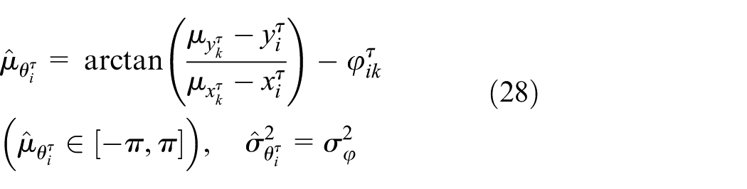
Unlike landmark, the estimation of robot node’s state still includes orientation angle other than position. As we can see in equation (26), based on the position of $L_k^{\tau }$ and corresponding robot–landmark measurements $Z_{\mathrm{ik}}^{\tau }$ , the distribution over $X_i^{\tau }$ is decomposed into two marginal distributions of its position and orientation apart in the second step, wherein the determination of orientation ${\theta }_i^{\tau }$ requires the robot’s position information as one of preconditions; finally, inspired by Caceres et al., ²⁶ this type of message can be represented in a parametric form as the third step.

The distribution over robot’s position in 2D space is regarded as the circular distribution $C(x_i^{\tau },y_i^{\tau };{\mu }_C,r_C,{\Sigma }_C)$ , where the center of this circle is the position of observed landmark ${\mu }_C={\mu }_{L_k^{\tau }}$ , radius is relative range value $r_C=d_{\mathrm{ik}}^{\tau }$ , variance reflects the width of this ring ${\Sigma }_C={\Sigma }_{L_k^{\tau }}+{\sigma }_d^{2}E$ (E is the identity matrix). The pdf of this distribution is presented analytically

$$\begin{array}{c}{p}_C(p_{X_i^{\tau }};{\mu }_C,r_C,{\Sigma }_C)\propto \exp \hfill \\ [-\frac{1}{2}{(\hat{p}-r_C\frac{\hat{p}}{\Vert \hat{p}\Vert })}^{\mathrm{T}}{{\Sigma }_C}^{-1}(\hat{p}-r_C\frac{\hat{p}}{\Vert \hat{p}\Vert })]\hfill \end{array}$$

(27)

where $p_{X_i^{\tau }}=[x_i^{\tau },y_i^{\tau }{]}^{\mathrm{T}}$ , $\hat{p}=p_{X_i^{\tau }}-{\mu }_C$ and the symbol ||·|| denotes the Euclidean norm. Readers can refer to Caceres et al. ²⁶ for more details on this kind of distribution family.

The pdf of robot’s orientation obeys Gaussian distribution $N({\theta }_i^{\tau };{\hat{\mu }}_{{\theta }_i^{\tau }},{\hat{\sigma }}_{{\theta }_i^{\tau }}^2)$ after its position is estimated, with

$$\begin{array}{c}{\hat{\mu }}_{{\theta }_i^{\tau }}=\arctan \left(\frac{{\mu }_{y_k^{\tau }}-y_i^{\tau }}{{\mu }_{x_k^{\tau }}-x_i^{\tau }}\right)-{\phi }_{\mathrm{ik}}^{\tau }\hfill \\ ({\hat{\mu }}_{{\theta }_i^{\tau }}\in [-\pi ,\pi ]),{\hat{\sigma }}_{{\theta }_i^{\tau }}^2={\sigma }_{\phi }^2\hfill \end{array}$$

(28)

• 5. Message from robot–robot factor to robot variable $m_{h_{\mathrm{ij}}\to X_i}(X_i^{\tau })$

$$m_{h_{\mathrm{ij}}\to X_i}\left(X_i^{\tau }\right)=\sum _{X_j^{\tau }}{h}_{\mathrm{ij}}(X_i^{\tau },X_j^{\tau })m_{X_j\to h_{\mathrm{ij}}}\left(X_j^{\tau }\right)$$

(29)

In accordance with different observation cases and factor expressions (12)–(14), this message is discussed under three conditions. The first is pairwise mutual observation corresponding to equation (12) and can be written as

$$\begin{array}{cc}\multicolumn{1}{c}{m_{h_{\mathrm{ij}}\to X_i}\left(X_i^{\tau }\right)}& =p(X_i^{\tau }|X_j^{\tau },Z_{\mathrm{ij}}^{\tau },Z_{\mathrm{ji}}^{\tau })\hfill \\ \multicolumn{1}{c}{}& =N(X_i^{\tau };{\stackrel{⌢}{\mu }}_{X_i^{\tau }},{\stackrel{⌢}{\Sigma }}_{X_i^{\tau }})\hfill \end{array}$$

(30)

At this point, based on measurements of two sides $Z_{\mathrm{ij}}^{\tau }=[d_{\mathrm{ij}}^{\tau },{\phi }_{\mathrm{ij}}^{\tau }]$ , $Z_{\mathrm{ji}}^{\tau }=[d_{\mathrm{ji}}^{\tau },{\phi }_{\mathrm{ji}}^{\tau }]$ and the distribution of X_j, that is, $m_{X_j\to h_{\mathrm{ij}}}(X_j^{\tau })\approx N(X_j^{\tau };{\mu }_{X_j^{\tau }},{\Sigma }_{X_j^{\tau }})$ , the state of X_i is computed with

$$\begin{array}{c}{\stackrel{⌢}{\mu }}_{X_i^{\tau }}=\left[\begin{array}{c}{\stackrel{⌢}{\mu }}_{x_i^{\tau }}\hfill \\ \multicolumn{1}{c}{{\stackrel{⌢}{\mu }}_{y_i^{\tau }}}\\ \multicolumn{1}{c}{{\stackrel{⌢}{\mu }}_{{\theta }_i^{\tau }}}\end{array}\right]=\left[\begin{array}{c}{\mu }_{x_j^{\tau }}+\cos ({\phi }_{\mathrm{ji}}^{\tau }+{\theta }_j^{\tau })·(d_{\mathrm{ij}}^{\tau }+d_{\mathrm{ji}}^{\tau })/2\hfill \\ \multicolumn{1}{c}{{\mu }_{y_j^{\tau }}+\sin ({\phi }_{\mathrm{ji}}^{\tau }+{\theta }_j^{\tau })·(d_{\mathrm{ij}}^{\tau }+d_{\mathrm{ji}}^{\tau })/2}\\ \multicolumn{1}{c}{{\mu }_{{\theta }_j^{\tau }}+{\phi }_{\mathrm{ji}}-{\phi }_{\mathrm{ij}}+\pi }\end{array}\right]\hfill \\ ({\stackrel{⌢}{\mu }}_{{\theta }_i^{\tau }},{\mu }_{{\theta }_j^{\tau }}\in [-\pi ,\pi ])\hfill \end{array}$$

(31)

$${\stackrel{⌢}{\Sigma }}_{X_i^{\tau }}={\Sigma }_{X_j^{\tau }}+F{\Sigma }_{\mathrm{obs}}{F}^{\mathrm{T}}$$

(32)

The second one corresponding to equation (13) is one-way relationship that X_i can see peer X_j but the inverse is not; the third case corresponding to equation (14) is the contrary of the second. The solution to these two is similar to message (4) written by the joint of circular distribution regarding position and Gaussian distribution regarding orientation angle, so they would not be covered here.

• 6. Message from landmark variable to robot–landmark factor ${m_{L_k\to }}_{g_{\mathrm{ik}}}(L_k^{\tau })$

$${m_{L_k\to }}_{g_{\mathrm{ik}}}(L_k^{\tau })\propto m_{f_{L_k}\to L_k}(L_k^{\tau })\underset{X_j^{\tau }\in N_k^{\tau }/X_i^{\tau }}{\Pi }{m}_{g_{\mathrm{jk}}\to L_k}(L_k^{\tau })$$

(33)

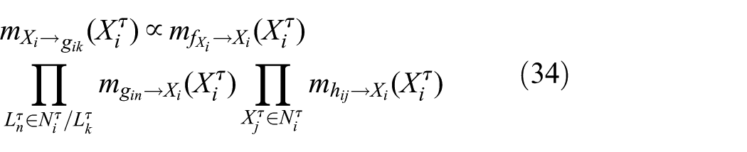
• 7. Messages from robot variable to robot–landmark factor ${m_{X_i\to }}_{g_{\mathrm{ik}}}(X_i^{\tau })$

$$\begin{array}{c}{m_{X_i\to }}_{g_{\mathrm{ik}}}(X_i^{\tau })\propto m_{f_{X_i}\to X_i}(X_i^{\tau })\hfill \\ \underset{L_n^{\tau }\in N_i^{\tau }/L_k^{\tau }}{\Pi }{m}_{g_{\mathrm{in}}\to X_i}(X_i^{\tau })\underset{X_j^{\tau }\in N_i^{\tau }}{\Pi }{m}_{h_{\mathrm{ij}}\to X_i}(X_i^{\tau })\hfill \end{array}$$

(34)

• 8. Messages from robot variable to robot–robot factor ${m_{X_i\to }}_{h_{\mathrm{ij}}}(X_i^{\tau })$

$$\begin{array}{c}{m_{X_i\to }}_{h_{\mathrm{ij}}}(X_i^{\tau })\propto m_{f_{X_i}\to X_i}(X_i^{\tau })\underset{L_k^{\tau }\in N_i^{\tau }}{\Pi }{m}_{g_{\mathrm{ik}}\to X_i}(X_i^{\tau })\hfill \\ \underset{X_n^{\tau }\in N_i^{\tau }/X_j^{\tau }}{\Pi }{m}_{h_{\mathrm{in}}\to X_i}(X_i^{\tau })\hfill \end{array}$$

(35)

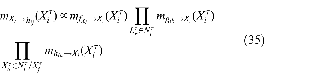
The last three types of messages are determined by the product of incoming parametric messages whose types belong to messages (1)–(5). However, it is not analytically tractable to calculate these complex outgoing messages owing to mixed distribution forms and changeful quantity of incoming messages. Hence, we attempt to use concise Gaussian distributions to approximate the resulting nonparametric messages, which converts this problem to seeking optimal parameters characterize these output distributions. Enlightened from PF, ³² we put forward a hybrid information fusion algorithm for such a purpose. In a nutshell, this algorithm employs the sampling method: samples are taken from Gaussian distribution of prediction message which offers preliminary state estimation of variable node in terms of physical model, and then, put into analytical distributions corresponding to remaining incoming messages to produce probability density values, whose product could determine an attached weight; using weighted samples, outgoing distribution is more accurately estimated. Next, message (8) will be set as an example to illustrate the above procedures summarized in Algorithm 1, and messages (6) and (7) can be deduced from this.

Algorithm 1: Hybrid parametric and nonparametric information fusion—message (8) version
Input:	Distributions of all incoming messages
Output:	Parameters of message ${m_{X_i\to }}_{h_{\mathrm{ij}}}(X_i^{\tau })\approx N(X_i^{\tau };{\tilde{\mu }}_{X_i^{\tau }},{\tilde{\Sigma }}_{X_i^{\tau }})$
1	Draw S samples $\{{\tilde{X}}_{i,s}^{\tau }{\}}_{s=1}^S$ from prediction message $m_{f_{X_i}\to X_i}(X_i^{\tau })$
2	Weight each of S samples by $w_s=\underset{L_k^{\tau }\in N_i^{\tau }}{\Pi }{m}_{g_{\mathrm{ik}}\to X_i}({\tilde{X}}_{i,s}^{\tau })\underset{X_n^{\tau }\in N_i^{\tau }/X_j^{\tau }}{\Pi }{m}_{h_{\mathrm{in}}\to X_i}({\tilde{X}}_{i,s}^{\tau })$
3	Normalize weights such that $\sum _{s=1}^S{w}_s=1$
4	Calculate mean ${\tilde{\mu }}_{X_i^{\tau }}$ and covariance ${\tilde{\Sigma }}_{X_i^{\tau }}$ of outgoing distribution by weighted samples ${\tilde{\mu }}_{X_i^{\tau }}=\sum _{s=1}^S{w}_s{\tilde{X}}_{i,s}^{\tau }{\tilde{\Sigma }}_{X_i^{\tau }}=\frac{\sum _{s=1}^S{w}_s({\tilde{X}}_{i,s}^{\tau }-{\tilde{\mu }}_{X_i^{\tau }}){({\tilde{X}}_{i,s}^{\tau }-{\tilde{\mu }}_{X_i^{\tau }})}^{\mathrm{T}}}{1-\sum _{s=1}^S{w}_s^2}$

Belief calculation

Belief $b(X_i)$ (or $b(L_k)$ ), as a estimated marginal probability, is computed by the product of all incoming messages to variable node $X_i$ (or $L_k$ ), whose update relies on message passing between variable and factor nodes in BP algorithm. At every timestep, updating belief state of each variable node needs iterative calculation process, which is often initialized using distributions of prediction message, that is

$$m_{{L_k\to }_{g_{\mathrm{ik}}}}^0(L_k^{\tau })=m_{f_{L_k}\to L_k}(L_k^{\tau })$$

(36)

$$m_{{X_i\to }_{g_{\mathrm{ik}}}}^0(X_i^{\tau })=m_{f_{X_i}\to X_i}(X_i^{\tau })$$

(37)

$$m_{{X_i\to }_{h_{\mathrm{ij}}}}^0(X_i^{\tau })=m_{f_{X_i}\to X_i}(X_i^{\tau })$$

(38)

In the rth iteration, the calculation of the messages from factor nodes to variable nodes is the first step

$$m_{g_{\mathrm{ik}}\to L_k}^r\left(L_k^{\tau }\right)\propto \sum _{X_i^{\tau }}{g}_{\mathrm{ik}}(X_i^{\tau },L_k^{\tau })m_{X_i\to g_{\mathrm{ik}}}^{r-1}\left(X_i^{\tau }\right)(L_k^{\tau }\in N_i^{\tau })$$

(39)

$$m_{g_{\mathrm{ik}}\to X_i}^r\left(X_i^{\tau }\right)\propto \sum _{L_k^{\tau }}{g}_{\mathrm{ik}}(X_i^{\tau },L_k^{\tau })m_{L_k\to g_{\mathrm{ik}}}^{r-1}\left(L_k^{\tau }\right)(L_k^{\tau }\in N_i^{\tau })$$

(40)

$$m_{h_{\mathrm{ij}}\to X_i}^r\left(X_i^{\tau }\right)\propto \sum _{X_j^{\tau }}{h}_{\mathrm{ij}}(X_i^{\tau },X_j^{\tau })m_{X_j\to h_{\mathrm{ij}}}^{r-1}\left(X_j^{\tau }\right)(X_j^{\tau }\in N_i^{\tau })$$

(41)

what follows is the calculation of variable-to-factor messages, which can be broadcast in the beginning of next iteration

$$m_{L_k\to g_{\mathrm{ik}}}^r(L_k^{\tau })\propto \underset{X_j^{\tau }\in N_k^{\tau }/X_i^{\tau }}{\Pi }{m}_{g_{\mathrm{jk}}\to L_k}^r(L_k^{\tau })$$

(42)

$$m_{X_i\to g_{\mathrm{ik}}}^r(X_i^{\tau })\propto \underset{L_n^{\tau }\in N_i^{\tau }/L_k^{\tau }}{\Pi }{m}_{g_{\mathrm{in}}\to X_i}^r(X_i^{\tau })\underset{X_j^{\tau }\in N_i^{\tau }}{\Pi }{m}_{h_{\mathrm{ij}}\to X_i}^r(X_i^{\tau })$$

(43)

$$m_{X_i\to h_{\mathrm{ij}}}^r(X_i^{\tau })\propto \underset{L_k^{\tau }\in N_i^{\tau }}{\Pi }{m}_{g_{\mathrm{ik}}\to X_i}^r(X_i^{\tau })\underset{X_n^{\tau }\in N_i^{\tau }/X_j^{\tau }}{\Pi }{m_{h_{\mathrm{in}}\to }^r}_{X_i}(X_i^{\tau })$$

(44)

After reaching the required number R of iterations, the belief of a mobile robot variable node at current timestep $\tau$ can be calculated by converging all messages from neighboring factors $f$ , $g$ , and $h$

$$b(X_i^{\tau })\propto m_{f_{X_i}\to X_i}(X_i^{\tau })\underset{L_k^{\tau }\in N_i^{\tau }}{\Pi }{m}_{g_{\mathrm{ik}}\to X_i}(X_i^{\tau })\underset{X_j^{\tau }\in N_i^{\tau }}{\Pi }{m}_{h_{\mathrm{ij}}\to X_i}(X_i^{\tau })$$

(45)

similarly, the belief of a landmark variable node is

$$b(L_k^{\tau })\propto m_{f{L}_k\to L_k}(L_k^{\tau })\underset{X_i^{\tau }\in N_k^{\tau }}{\Pi }{m}_{g_{\mathrm{ik}}\to L_k}(L_k^{\tau })$$

(46)

Concerning some isolated variable nodes whose neighboring factors only include prediction factors, their beliefs are directly obtained using prediction messages.

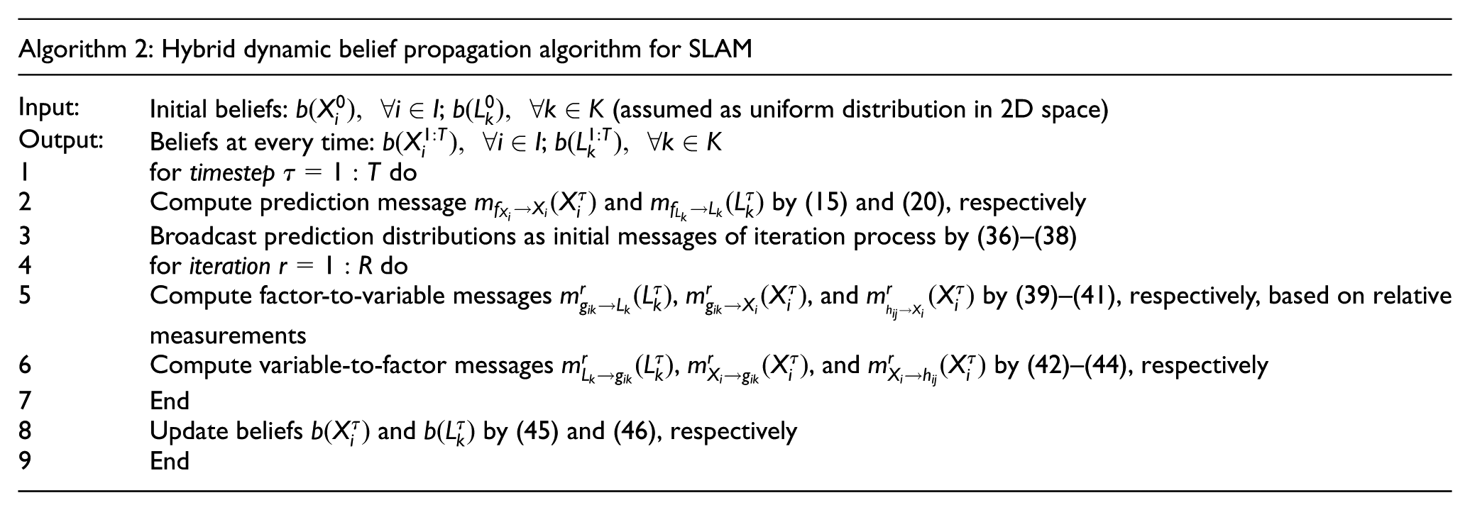
To sum up, we present the hybrid dynamic BP algorithm for SLAM, as designed in Algorithm 2. And we should notice that every variable node undertakes local information processing and computational burden, so this algorithm is fully distributed and available to large-scale robot fleets, even portable to other mobile sensor networks.

Algorithm 2: Hybrid dynamic belief propagation algorithm for SLAM
Input:	Initial beliefs: $b(X_i^0),\forall i\in I$ ; $b(L_k^0),\forall k\in K$ (assumed as uniform distribution in 2D space)
Output:	Beliefs at every time: $b(X_i^{1:T}),\forall i\in I$ ; $b(L_k^{1:T}),\forall k\in K$
1	for timestep $\tau =1:T$ do
2	Compute prediction message $m_{f_{X_i}\to X_i}(X_i^{\tau })$ and $m_{f_{L_k}\to L_k}(L_k^{\tau })$ by (15) and (20), respectively
3	Broadcast prediction distributions as initial messages of iteration process by (36)–(38)
4	for iteration $r=1:R$ do
5	Compute factor-to-variable messages $m_{g_{\mathrm{ik}}\to L_k}^r(L_k^{\tau })$ , $m_{g_{\mathrm{ik}}\to X_i}^r(X_i^{\tau })$ , and $m_{h_{\mathrm{ij}}\to X_i}^r(X_i^{\tau })$ by (39)–(41), respectively, based on relative measurements
6	Compute variable-to-factor messages $m_{L_k\to g_{\mathrm{ik}}}^r(L_k^{\tau })$ , $m_{X_i\to g_{\mathrm{ik}}}^r(X_i^{\tau })$ , and $m_{X_i\to h_{\mathrm{ij}}}^r(X_i^{\tau })$ by (42)–(44), respectively
7	End
8	Update beliefs $b(X_i^{\tau })$ and $b(L_k^{\tau })$ by (45) and (46), respectively
9	End

Message passing schedule

In this subsection, we will expound the process and additional items of message passing although its rough framework has been exhibited in the previous subsection. In Algorithm 2, there are two temporal work patterns: for the timestep pattern, new measurements can be utilized; for the iteration pattern, measurements used to update messages remain constant. To perform the whole evolution clearly, we define a message passing matrix M_pass to describe the situation of synchronous message broadcasting during each iteration.

M_pass is a (I + K)-by-(I + K) matrix, whose contents are updated with every iteration. Its basic format is shaped like Table 2, which represents the situation about initial messages of iteration process corresponding to the SLAM scenario in Figure 5; some explanations for M_pass are made as below:

• I mobile robots are denoted by the first I label indexes, after the K labels denote K landmarks, for instance, labels 1–5 are robots and 6–15 are landmarks in Table 2.

• Elements A denote messages from variables to factor nodes, that is, message types (6)–(8), which are sent from objects appearing in the row labels to column labels involved in related factors of messages at the beginning of next iteration, and located in blocks lower left K-by-I, upper right I-by-K, and upper left I-by-I, respectively.

• Only when the observation relationship exists between two objects at this timestep might elements linking with bound labels of those two have values A after every iteration; in other words, elements × show that linked two objects are impossible to create observations at any time, and elements null show that linked two objects have no observations at this time, or unsatisfied conditions for message broadcasting despite real observations.

• Only robots and landmarks whose position estimation variances satisfy the following condition can send messages to neighbor factors; since relatively inaccurate landmarks could result in the divergence of positioning errors accumulating over time throughout the entire network, a variance threshold ξ is imposed to judge whether some observed landmark can broadcast messages, then in virtue of observation noise variance ${\sigma }_d^2$ , when current covariance ${\Sigma }_{L_k^{\tau }}$ of the landmark meets

$$\sum _{L_k^{\tau }}(\mathrm{ind},\mathrm{ind})\in {\sigma }_d^2\pm \xi (\mathrm{ind}=1,2)$$

(47)

this landmark satisfies the condition for message broadcasting, that is, there are values in corresponding elements.

• In order to further enhance the algorithm performance, some rules are also permitted to comply, for example, only when message number received by some column reaches a minimum does the object corresponding to this column label qualify for broadcasting messages at next iteration.

Table 2.

Message passing matrix M⁰ _pass corresponding to initial iteration situation of Figure 5.

Figure 5.

Typical example of multi-robot SLAM scenario at some timestep τ. There are five robots indexed as numbers 1–5 and 10 landmarks indexed as numbers 6–15.

At the end of this subsection, using M_pass and assuming iteration number R = 2 at this timestep, we complete message passing procedures for the scenario example in Figure 5. At time τ, all object variables participating in observation events should have broadcast messages to neighbor factors in the initial situation M⁰ _pass calculated by (36)–(38) of all iteration loops, but we could see that no values exist in the 12–14th lines of Table 2, that is, current position estimations of landmarks 12, 13, and 14 are so inaccurate that these landmarks dissatisfy the aforementioned condition for message broadcasting at the beginning of next iteration.

Using messages in M⁰ _pass and executing statements 5–6 for the first iteration in Algorithm 2, we can obtain M¹ _pass showed in Table 3. For landmark 7 receiving a message from robot 2 in M⁰ _pass , we use equations (36) and (39) to get $m_{L_7\to g_{27}}^1$ , and find that the variance of current estimation brought by $m_{L_7\to g_{27}}^1$ exceeds the limit (47), so this message cannot be broadcast by landmark 7 at the beginning of next iteration, that is, $m_{L_7\to g_{27}}^1$ cannot be written as $A_{27}^1$ existing in M¹ _pass ,; similar situations happen to landmarks 8, 11, and 12. Differently, landmarks 9, 13, and 14 fit the bill, so they with robots will broadcast messages at next iteration.

Table 3.

Message passing matrix M¹ _pass corresponding to the first iteration of Figure 5.

Procedures same as the last iteration are implemented and then we can obtain M² _pass in Table 4. So far, we have finished all iterative loops; then based on messages in M² _pass , the belief states at this time τ can be calculated using equations (45) and (46).

Table 4.

Message passing matrix M² _pass corresponding to the second iteration of Figure 5.

Results

This section elaborates the simulation and comparison experiment conducted with MATLAB to verify the performance of our algorithm. In the above two kinds of experiments, we adopt the mean position estimate error (between estimated value and ground truth), that is, root mean square error (RMSE), as evaluation criterion in unison, which is defined as

$$\begin{array}{c}M{E}_{X_i}\left(\tau \right)=\Vert {\stackrel{·}{p}}_{X_i^{\tau }}-p_{X_i^{\tau }}\Vert (\forall i\in I)\hfill \\ M{E}_X\left(\tau \right)=\frac{1}{I}\sum _{i=1}^I\Vert {\stackrel{·}{p}}_{X_i^{\tau }}-p_{X_i^{\tau }}\Vert \hfill \\ M{E}_L\left(\tau \right)=\frac{1}{K}\sum _{k=1}^K\Vert {\stackrel{·}{L}}_k^{\tau }-L_k^{\tau }\Vert \hfill \end{array}$$

Simulation results

In this part, we will implement our method using simulation data to simply testify its feasibility and effectiveness. The simulation scene, shown in Figure 6, and corresponding parameter configuration are described as follows:

• In total, 15 landmarks are deployed randomly and manually on the 2D space with an area 10 m × 10 m, and real trajectories of three mobile robots are planned by MATLAB built-in functions, ginput and spline.

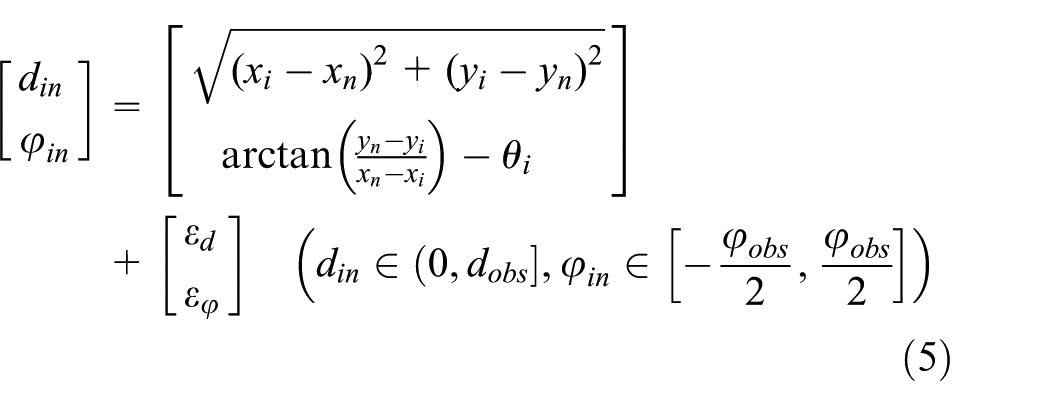
• Required ground truth data are fetched by path sampling every 0.1 s, that is, per timestep = 0.1 s, then odometry data are obtained by dint of a series of discrete sampled waypoints, and measurements are made using equation (5) at every timestep.

• Some model parameters are setting as ${\sigma }_v=0.2\mathrm{m}/\mathrm{s}$ , ${\sigma }_{\omega }=0.3\mathrm{rad}/\mathrm{s}$ , $d_{\mathrm{obs}}=4\mathrm{m}$ , ${\phi }_{\mathrm{obs}}=\pi /3(\pm \pi /6)$ , ${\sigma }_d=0.2\mathrm{m}$ , and ${\sigma }_{\phi }=0.05\mathrm{rad}$ .

• The number of samples S = 1000 in Algorithm 1, iteration loops R = 2 per timestep in Algorithm 2, and variance threshold $\xi =0.015$ in message passing scheme.

Figure 6.

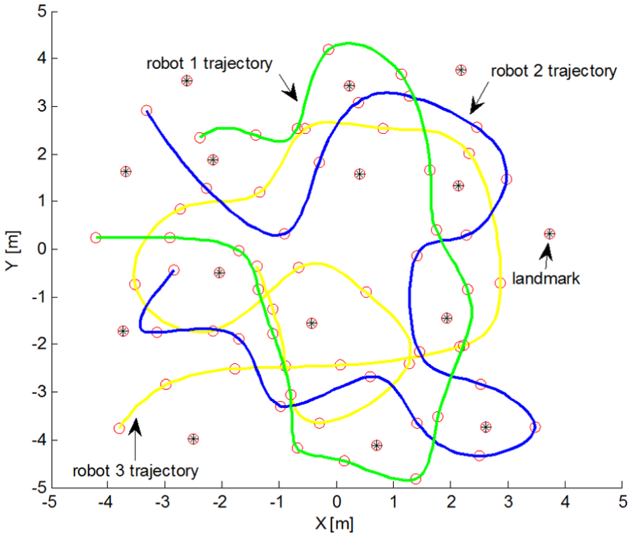
Simulation scene with 3 mobile robots and 15 landmarks. Landmarks marked with black asterisks are placed randomly and their position coordinates can be returned by MATLAB function ginput. In the same way, the robot trajectories marked with color curves are outlined by some random dots marked with red circles.

With the above settings and known initial states of robots, simulation results during the duration of the first 180 s are depicted in Figure 7. In the earlier period, there is rather larger position error for landmarks because of scanty measurements produced by robots; with the progression of time, more and more landmarks are gradually observed by mobile robots, meanwhile, participate in message passing to constantly correct and update own belief states; after 130 s or so, all landmarks should be observed and their position error converges to the minimum, that is, they are localized relatively exactly at this point. For mobile robots, their position estimation has kept high accuracy in the whole duration. These results directly reflect the validity of our distributed algorithm; in terms of hybrid information fusion, parameterization ensures computation speed, while nonparameterization technique can indeed approximate arbitrary probability distributions.

Figure 7.

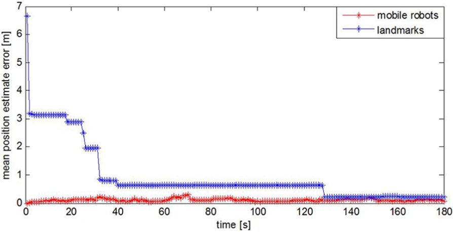
Simulation results about objects’ mean position estimate error.

Experimental results

Furthermore, the performance of our algorithm is compared on publicly available dataset ⁷ with its founders’ decentralized EKF-SLAM method for dynamic and sparse robot networks in Leung et al., ¹⁰ where each robot obtains the exact centralized-equivalent estimates for all robot poses and the positions for all known landmarks in a decentralized manner. In the decentralized EKF-SLAM, every robot possesses a knowledge set comprising all odometry and measurement data, as well as the previous state estimates known to itself at every time; when communication occurs between robots i and j, they will make their knowledge sets available to each other, that is, the knowledge set of both robots will become identical; based on above knowledge sets, any recursive approximation of the Bayes filter, such as EKF, here, will be used to produce the current state estimates.

The public MR.CLAM dataset, ⁷ provided by the University of Toronto Institute for Aerospace Studies (UTIAS), is generated using five mobile robots in an indoor 15 m × 8 m space with 15 static landmarks, each of which has a unique identification number encoded as a barcode. This dataset consists of nine sub-datasets, whose real environment has been shortly shown in Figure 1, and sensing device has been introduced in section “Problem formulation.” Keeping in step with the Leung et al., ¹⁰ we thus choose sub-dataset 1 for comparison due to its sparsest connecting and communicating network of all the datasets, which is produced through a 25-min hardware experiment, wherein some useful features are the following:

• Individual landmarks are scattered randomly throughout the workspace, and robots are also initially placed randomly in the workspace.

• Each robot logs its own odometry data while driving to randomly generated waypoints in the workspace and avoiding other objects.

• Ground truth data of all robot poses $(x,y,\theta )$ and all landmark position $(x,y)$ for all times are offered with positional accuracy of the order of 1 × 10⁻³ m, which are rarely available for SLAM experiments.

• The maximum forward velocity of a robot is 0.16 m/s, the maximum angular velocity is 0.35 rad/s, and each camera has a field of view of approximately 60°.

• A measurement range limit can be imposed by ignoring measurements that exceed a custom range, and truth data are permitted to sample at a fixed frequency.

Consequently, we can set path sampling frequency as 0.2 s, that is, per timestep = 0.2 s; besides, other model and algorithm parameters are coincidence with those of simulation.

Figure 8 shows the landmarks’ mean position estimate error variation versus time. In the first 70 s, with mobile sensors probing the surroundings, landmarks are gradually observed and more and more usable measurements are generated, so position estimate errors of two methods are decreased continuously. After 70 s, we can see that two curves tend to keep stable for a long time, each of which converges to a certain value. That is, at this moment all landmarks should be seen and located and the steady convergence error value reflects the positioning accuracy, which is about 0.2 m for our algorithm, but 0.7 m or so for comparison method. It is clear that our method outperforms that one in positioning accuracy although they exhibit little difference on convergent speed. This is attributed to the fact that, our method can flexibly approximate different probability distributions using nonparametric technique, which is better to solve nonlinear problems in modeling and measuring process. In contrast, in order to transform nonlinear problems into linear ones, EKF neglects higher-order terms of Taylor series expansion except its first-order term in general, which introduces comparatively large errors and somewhat more seriously, results in filter divergence.

Figure 8.

RMSE of landmarks versus time.

When realizing landmarks’ positioning, we draw 500 samples from the probability distribution of every landmark state, respectively, to visualize state estimation results in Figure 9, which also displays every landmark real position marked with the blue asterisk and estimated mean positions obtained in both methods. The sampling points generated by our algorithm can cover the landmarks real positions better. That is, our estimated mean position is closer to, and even coincides with its truth value, like landmark 5, 10, and 11. By comparison, there are relatively larger deviations between mean positions estimated by decentralized EKF-SLAM method and their respective truth values. Like landmark 1, 2, 3, 4, 5, 9, and 14, their true positions even fall out of scope covered by samples generated from comparison method.

Figure 9.

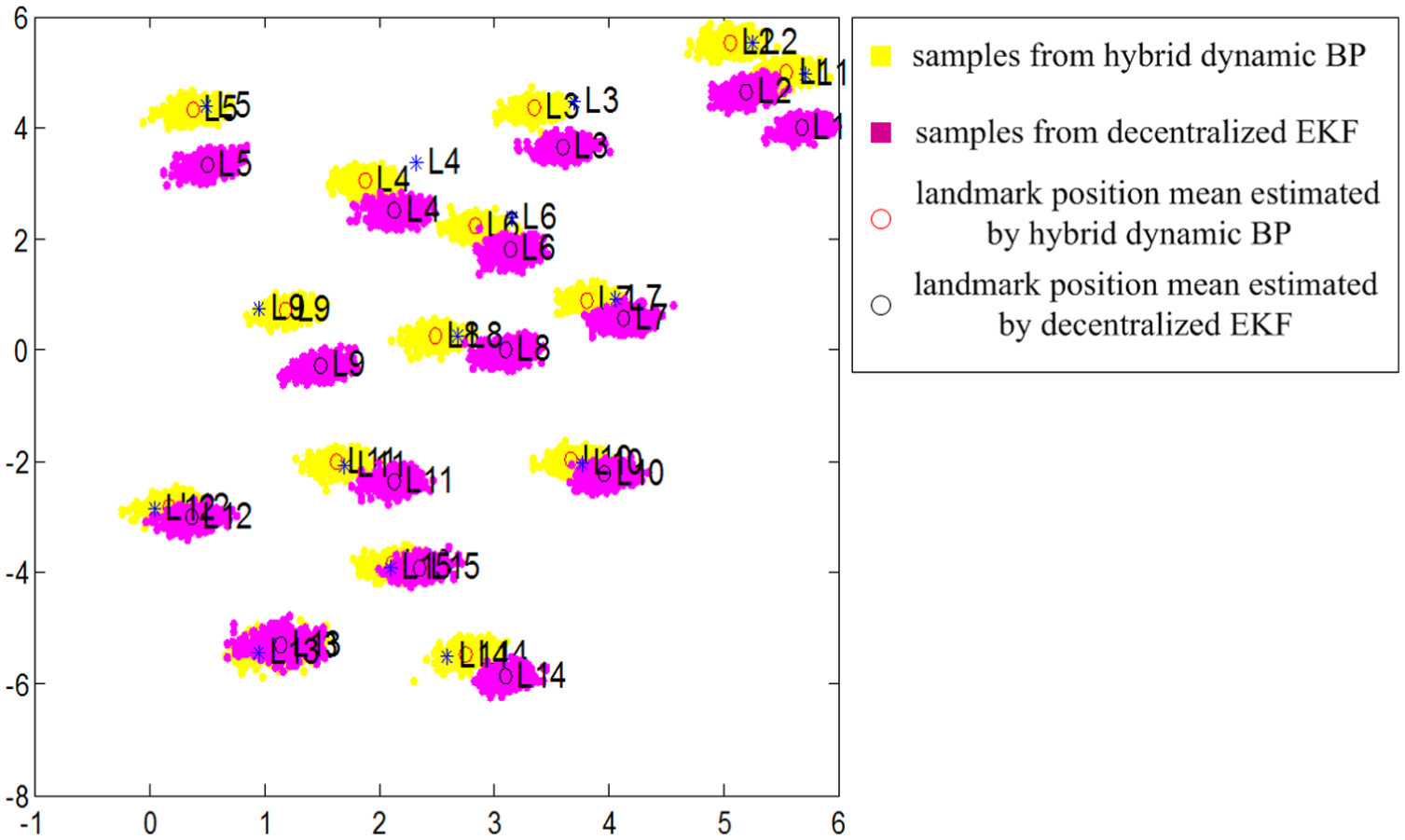
Posterior probability distribution for the location of every landmark.

In the context that initial states of all robots are known, every robot’s position estimate error variation versus time is acquired in Figure 10. Every robot’s mean position estimate error obtained by our algorithm is about 0.2 m, but for the other method, this kind of error is pretty large. Moreover, error variation curves pertaining to contrastive method have rather bigger fluctuation; in other words, decentralized EKF-SLAM method has worse positioning stability. We also take note of the case that in the curves from our algorithm, relatively greater position error appears at certain times, for example, in the period from 200 to 400 s for robot 2. Actually, it is inevitable that the connection among nodes in some local networks can be sparse because of robots’ free movement, which results in the decrease in available observations and thus influences positioning accuracy. However, making full use of landmarks located as reference to correct accumulated error brought by odometer (according to Figure 8, note that the task, locating all landmarks, was accomplished at about 70 s), our algorithm still keep positioning accuracy superior to the other one in such case.

Figure 10.

Position estimate error of every robot versus time.

Beside the inherent limitation of EKF mentioned before, the fact that the centralized-equivalent estimates may be delayed as robots wait for required information to arrive over the sparse network is also a cause of underperformance of decentralized EKF-SLAM method. So, backed by last known odometry and other available information in the knowledge set, temporary estimates are produced as the current state estimate until communication is reestablished and centralized-equivalent estimates are recovered, which could have temporary estimates diverge from the real robot pose. At the same time, in order to prevent from the problems of inadequate memory space and cyclical state renewal, applying Markov property is helpful to remove historical data that are no longer needed in knowledge sets, which leads into a range of issues needed to confirm accordingly, for instance, how to find the right checkpoint in time to apply Markov property. However, from message passing point of view, what is propagated between nodes in our algorithm is, at bottom, only estimated state of the involved variable node, which easily avoids to take data delay and circulated update problems into account.

Conclusion

In this article, we propose a hybrid dynamic BP algorithm to solve SLAM problem of mobile robot networks in the unknown environment represented by discriminable landmarks whose positions are unknown. It is crucial to recursively estimate the positions of landmarks and all robot poses using odometry data and observation information. Based on the independence among moving robots, Markov property of motion model and Bayesian theory, we factorize the joint posterior probability distribution of all landmark and robot variables and model a factor graph to make probabilistic inference, wherein local information processing and exchanging can make sure that our algorithm is implemented in a distributed manner. Furthermore, we detail message calculation and passing, and apply hybrid dynamic BP to determine the belief state of every variable. Necessarily, we carry out simulations and comparison experiments to demonstrate the effectiveness and accuracy. In the future, we will study the more complicated SLAM problem under the case that the detected environment is completely unknown, which means that landmarks are indistinguishable.