The mine locomotive wireless network strategy based on successive interference cancellation with dynamic power control

Abstract

Mine locomotives are widely used in mining industry for transporting. Usually, these locomotives need to move along the tunnels and communicate with access points which are equipped on the side of these tunnels. It is important to maintain high-quality communication services due to the unsafe underground working environment. In this article, we design the mine locomotive wireless network strategy based on successive interference cancellation with dynamical power control. We first divide the whole schedule time into time segments and build the problem model in each time segment. To maximize throughput for each time segment, we formulate a linear programming problem based on certain features of successive interference cancellation decoding order. However, this problem has lots of constraints which makes it hard to solve in polynomial time. Then, we propose a concept of the maximum successive interference cancellation set to reduce the problem size. Based on this concept, we propose a polynomial complexity algorithm named max-SIC-set algorithm. Simulation results show that our algorithm can increase throughput significantly compared with the algorithm using successive interference cancellation only (no power control) and with the algorithm without using successive interference cancellation and power control.

Introduction

Mine locomotives are widely used in mining industry for transporting. Usually, the mine locomotives are needed to be driven by men when they travel along the underground tunnels. However, the underground working environment is a harsh environment. According to incomplete statistics, at least 50,000 miners lost their lives from 2001 to 2014 in China. ¹ Among all kinds of these incidents, at least $30\%$ are caused by transporting systems. Fortunately, with the development of technology, the death rate decreased significantly. For example, in China, the number of death miners is 5670 in 2001 while is 931 in 2014. ² But 931 is still a big number, and if we can make the transporting systems safer, then lots of lives may not be lost.

Nowadays, we usually use some mine locomotive systems to control and regulate the mine locomotives, such as the signal centralization interlocking system. ³ A typical mine locomotive system (see Figure 1) is usually consisted with underground locomotives, access points (APs), and the ground control center. The underground locomotives will transmit their data to APs and then APs will forward data to the ground control center. The APs can use wired networks to transform data to the ground control center. But, locomotives are mobile, and thus, it is better for them to transmit their data to APs by wireless networks. However, such a wireless network is not available in the traditional systems. So, data collection is done at the APs manually. ³

Figure 1.

A typical mine locomotive system.

Today, we can consider to use wireless network in the underground tunnels. Many researchers have done their work to improve transporting systems based on wireless network,^4,5 such as building monitoring systems for mine locomotives. ⁶ When using these improved transporting systems, locomotive data should be transmitted to APs efficiently and correctly. Especially to unmanned locomotive systems, the locomotive may transmit image or video data to APs by wireless network, which means we need to design robust transporting systems with large capacity. Nowadays, the wireless network protocols used in underground tunnels do not have many differences with which used in vehicular ad hoc network (VANET).^7,8 Since, in wireless network, collisions often happen when several transmitters are transmitting together, traditional schemes will force the transmitters to abandon the transmitting data and wait for transmitting again. This is not an efficient way to underground wireless network.

Unlike the traditional schemes, some other technologies can let several transmitters transmitting simultaneously, and these technologies are more suitable for the underground locomotive wireless network. For example, successive interference cancellation (SIC) is a typical protocol^9,10 of this type. Because of its good performance and easy implementation, SIC has been widely used. Its basic principle can be described as follows. When combined data with several transmitters’ information are received by a receiver, it will first try to decode and receive the strongest signal from the combined data. Only when the Shannon capacity is satisfied, the strongest signal can be decoded. After doing this, the strongest signal can be removed from the combined data, and the receiver will try to decode the second strongest signal. This process will be proceeded until all signals are decoded or one signal cannot be decoded.

The rest of the article is organized as follows. In section “Related works” related works are discussed. In section “Mine locomotive wireless networks,” we describe the problem and show that it is a non-linear programming (NLP) formulation. We further show how to reformulate it as a linear programming (LP) problem. In section “Polynomial-time algorithm,” we design a polynomial-time algorithm based on the concept of maximum SIC set. In section “Simulation results,” simulation results show that our algorithm can achieve large throughput improvement than schemes without power control and SIC. Finally, conclusions are provided in section “Conclusion.” (An abridged version of this article has appeared in wireless algorithms, systems, and applications (WASA) 2016, Bozeman, MT, USA.) ¹¹

Related works

Many works have been done for underground mine systems. Most of them focus on positioning,^12,13 monitoring,^14,15 and unmanned locomotive systems. ¹⁶ And most just consider the wireless network protocols the same as which used in VANET.^8,9 The IEEE 802.11p, which is standardized as the medium access control (MAC) layer of the dedicated short-range communication (DSRC) standard, ¹⁷ is the most commonly used protocol in VANET.^18,19 It divides the whole bandwidth into seven channels; among them, one for exchanging control and safety-related messages and the other six for exchanging normal data. In the work by Yao et al., ¹⁷ the authors analyze the models for the safety-critical messages transmitting in the first channel and improve the existing work by taking several aspects into design consideration. In the work by Amadeo et al., ²⁰ the authors focus on the other six channels and propose the protocol named WAVE-based hybrid coordination function to improve performances of delay-constrained and loss-sensitive non-safety applications.

IEEE 802.11p is based on collision avoidance (CA), which means when collisions happen, the receiver will abandon the received data and ask transmitters to transmit again, while the interference management (IM)-based protocols ²¹ can let several transmitters transmitting simultaneously. IM is a realizing method for wireless network communication, and it can be categorized into several types, such as interference cancellation, ²² interference coordination, ²³ and interference randomization. ²³ In this article, we focus on the interference cancellation, which can be realized into several techniques further, such as SIC, ²⁴ parallel interference cancellation, ²⁵ and iterative interference cancellation. ²⁶ Among them, the SIC technique is preferred nowadays because of its good performance and easy implementation. Toumpis and Goldsmith’s ²⁷ work has proved that SIC technique can increase the capacity of wireless network significantly. Thus, we will use it in this article.

SIC changes the physical layer behaviors, so new schemes on the upper layer should be designed to fully exploit its capability. ²⁸ Many researchers have done their work in this research field. In the work by Shi et al., ²⁹ the authors proposed an optimal SIC scheme for one base station and one hop wireless network where they suppose that all transmitters’ positions are known and fixed. The throughput increased almost $100\%$ compared with the one without using SIC. In the work by Gelal et al., ³⁰ the authors proposed a framework that facilitates efficient multi-user MIMO-SIC enabled communications, and they named it MUSIC. The MUSIC is mainly focused on how to divide the whole wireless network into sub-topologies when using SIC, and simulation results show that MUSIC provided throughput improvements of up to four times. In the work by Jiang et al., ³¹ the authors designed an optimal algorithm for multi-hop ad hoc networks with SIC. Their algorithm is based on cross-layer design, that is, the algorithm designs both the transmitting scheme at link layer and the routing scheme at network layer. Simulation results show that the throughput can be increased by $47\%$ compared with the algorithm without using SIC. Based on the work of Jiang et al., ³¹ Shi et al. ³² proposed a greedy cross-layer algorithm with polynomial complexity for SIC in a multi-hop network. Their algorithm was more suitable for the network with large transmitting nodes. In our previous work, we have designed an optimal locomotive moving schedule for the underground locomotives via SIC with power control. ³³ In that work, we supposed that the tunnel is straight, with only one lane, and each locomotive’s working time can be allocated precisely.

Mine locomotive wireless networks

A mine locomotive wireless network provides communication support for locomotives by APs on the side of a straight tunnel (see Figure 2). These APs are deployed such that there is no overlap of APs’ coverage, and these APs cover the entire tunnel. Locomotives move along the tunnel and there may be multiple locomotives in an AP’s coverage at the same time. APs apply SIC ¹¹ to receive data from multiple locomotives. We want to maximize throughput for locomotives.

Figure 2.

The straight underground tunnel model.

Network model

We focus on the problem for one AP and locomotives within its coverage. The same approach can be applied to other APs. Suppose that each locomotive $l_i$ is in AP’s coverage for certain period of time $[t_i^s,t_i^e]$ and all these time periods are within $[0,T]$ . Each $l_i$ can apply power control and use power $p_i(t)\in [0,P]$ to transmit its data at time $t\in [t_i^s,t_i^e]$ .

To simplify discussions, we assume the coordinate of considered AP is zero and denote $x_i(t)$ as the coordinate of $l_i$ at time $t$ . Then, the distance between $l_i$ and AP at time $t$ is $d_i(t)=|x_i(t)|$ and propagation gain $g_i(t)=min\{(d_i(t){)}^{-\lambda },1\}$ , where $\lambda$ is the path loss index.

Now, we determine the communication range. Denote $N_0$ as noise and $\beta$ as the SINR (signal-to-interference-and-noise ratio) threshold for a successful transmission. The maximum transmission range $R_{max}$ is achieved when the transmission power is $P$ and there is no interference. Then, we have $(R_{max}{)}^{-\lambda }P/N_0=\beta$ , that is

$$R_{max}={\left(\frac{P}{N_0\beta }\right)}^{\frac{1}{\lambda }}$$

(1)

We define $R_{max}$ as a locomotive’s communication range since the transmission from $l_i$ may be successful only if $d_i(t)\le R_{max}$ . Then, the coordinate of $l_i$ is $x_i(t)=-R_{max}+v(t-t_i^s)$ , where $v$ is the locomotive speed.

A locomotive $l_i$ may not always transmit during $[t_i^s,t_i^e]$ . We denote binary variable ${\theta }_i(t)=1$ if $l_i$ transmits at time $t$ and ${\theta }_i(t)=0$ otherwise. Apparently, if ${\theta }_i(t)=0$ , we have $p_i(t)=0$ , that is

${\theta }_i(t)·P\ge p_i(t)(l_i\in N,t\in [0,T])$

where $N$ is the set of all locomotives.

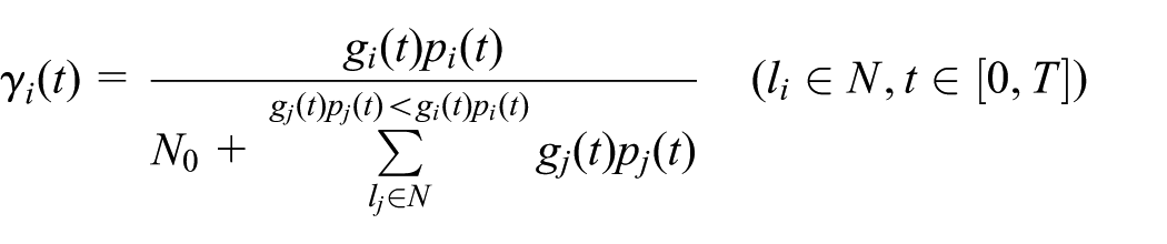
Under SIC, AP can receive multiple locomotives’ data simultaneously and decode them from the strongest signal to the weakest signal. ¹⁰ Once a signal is decoded, it will be canceled from the combined data, and thus, the SINR for the remaining signals increased. The SINR of $l_i$ at time $t$ under SIC can be written as

$${\gamma }_i(t)=\frac{g_i(t)p_i(t)}{N_0+\sum _{l_j\in N}^{g_j(t)p_j(t)<g_i(t)p_i(t)}{g}_j(t)p_j(t)}(l_i\in N,t\in [0,T])$$

The SINR requirement under SIC is if ${\theta }_i(t)=1$ , then ${\gamma }_i(t)\ge \beta$ , that is

$${\gamma }_i(t)\ge \beta ·{\theta }_i(t)(l_i\in N,t\in [0,T])$$

Problem formulation

In the last subsection, we describe constraints for a locomotive network with SIC. However, there are infinite number of variables, for example, ${\theta }_i(t)$ for $t\in [0,T]$ . In this section, we consider a problem based on SIC sets, where the SIC set is a set of locomotives that can transmit at the same time under SIC, and prove the existence of optimal solutions that satisfy a particular SIC decoding order. Then, we can formulate an NLP problem with finite number of variables.

To reduce the number of variables, we divide time $[0,T]$ into $m$ small time segments such that in each time segment, (1) the set of locomotives within AP’s coverage does not change, and (2) the distance between a locomotive in this set and the AP does not change much. Denote the set of time segments as $M$ . By (2), we can approximate the channel gain for a locomotive $l_i$ in time segment $k$ as a constant $g_{\mathrm{ik}}$ . Our objective is to maximize throughput in each time segment.

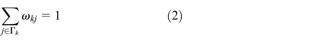
We now formulate an optimization problem for time segment $k$ . Given the set of locomotives within AP’s coverage, we can determine all SIC sets (by the approach in the next section). Denote ${\Gamma }_k$ as the set of SIC sets in time segment $k$ and $S_{\mathrm{kj}}$ as the $j\mathrm{th}$ SIC set in ${\Gamma }_k$ . We divide time segment $k$ into $|{\Gamma }_k|$ time slots and assign one time slot for each SIC set. Denote ${\tau }_{\mathrm{kj}}$ as the time slot assigned to $S_{\mathrm{kj}}$ and ${\omega }_{\mathrm{kj}}$ as the normalized length of time slot ${\tau }_{\mathrm{kj}}$ . We have

$$\sum _{j\in {\Gamma }_k}{\omega }_{\mathrm{kj}}=1$$

(2)

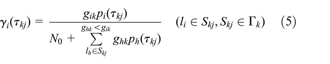
Since both the set of active locomotives and their channel gains do not change within a time slot, these locomotives do not need to change their transmission powers in a time slot. Denote $p_i({\tau }_{\mathrm{kj}})$ as the power of $l_i$ in time slot ${\tau }_{\mathrm{kj}}$ . The SINR for a locomotive $l_i$ in time slot ${\tau }_{\mathrm{kj}}$ is

$${\gamma }_i({\tau }_{\mathrm{kj}})=\frac{g_{\mathrm{ik}}{p}_i({\tau }_{\mathrm{kj}})}{N_0+\sum _{l_h\in S_{\mathrm{kj}}}^{g_{\mathrm{hk}}{p}_h({\tau }_{\mathrm{kj}})<g_{\mathrm{ik}}{p}_i({\tau }_{\mathrm{kj}})}{g}_{\mathrm{hk}}{p}_h({\tau }_{\mathrm{kj}})}(l_i\in S_{\mathrm{kj}},S_{\mathrm{kj}}\in {\Gamma }_k)$$

(3)

The SINR requirement under SIC is

$${\gamma }_i({\tau }_{\mathrm{kj}})\ge \beta (l_i\in S_{\mathrm{kj}},S_{\mathrm{kj}}\in {\Gamma }_k)$$

(4)

Note that in equation (3), the set of terms in $\sum _{l_h\in S_{\mathrm{kj}}}^{g_{\mathrm{hk}}{p}_h({\tau }_{\mathrm{kj}})<g_{\mathrm{ik}}{p}_i({\tau }_{\mathrm{kj}})}{g}_{\mathrm{hk}}{p}_h({\tau }_{\mathrm{kj}})$ depends on $p_h({\tau }_{\mathrm{kj}})$ and $p_i({\tau }_{\mathrm{kj}})$ values. But in a math programming formulation, the set of terms should be fixed. To resolve this issue, it is important to note that optimal solutions are not unique. Instead of considering all optimal solutions, we focus on optimal solutions with a particular SIC decoding order described in the following theorem.

Theorem 1. There is an optimal solution $\phi$ satisfying the following requirement: in each time slot, locomotives are decoded by the decreasing order of their channel gains to AP.

To prove Theorem 1, we first need the following corollary.

Corollary 1. Suppose that in an optimal solution $\hat{\phi }$ and a time slot ${\tau }_{\mathrm{kj}}$ , locomotive $l_h$ is decoded right after $l_i$ and $l_h$ ’s channel gain to AP is larger than $l_i$ ’s channel gain, where $l_h,l_i\in S_{\mathrm{kj}}$ . Then, there is another optimal solution $\phi$ with locomotive $l_i$ which is decoded right after $l_h$ in time slot ${\tau }_{\mathrm{kj}}$ .

Proof. Suppose that in solution $\hat{\phi }$ and time slot ${\tau }_{\mathrm{kj}}$ , transmission powers at $l_h$ and $l_i$ are ${\hat{p}}_h({\tau }_{\mathrm{kj}})$ and ${\hat{p}}_i({\tau }_{\mathrm{kj}})$ , respectively. We construct solution $\phi$ by letting $p_i({\tau }_{\mathrm{kj}})=g_{\mathrm{hk}}{\hat{p}}_h({\tau }_{\mathrm{kj}})/g_{\mathrm{ik}}$ and $p_h({\tau }_{\mathrm{kj}})=g_{\mathrm{ik}}{\hat{p}}_i({\tau }_{\mathrm{kj}})/g_{\mathrm{hk}}$ and keeping other variables’ values unchanged. Then, we have $g_{\mathrm{ik}}{p}_i({\tau }_{\mathrm{kj}})=g_{\mathrm{hk}}{\hat{p}}_h({\tau }_{\mathrm{kj}})$ and $g_{\mathrm{hk}}{p}_h({\tau }_{\mathrm{kj}})=g_{\mathrm{ik}}{\hat{p}}_i({\tau }_{\mathrm{kj}})$ , that is, received powers for $l_i$ and $l_h$ are switched. Thus, in solution $\phi$ , locomotive $l_i$ is decoded right after $l_h$ in time slot ${\tau }_{\mathrm{kj}}$ , that is, the constructed solution satisfies the requirement on SIC decoding order.

To show that solution $\phi$ is feasible, we only need to verify $p_i({\tau }_{\mathrm{kj}}),p_h({\tau }_{\mathrm{kj}})\le P$ . Since $g_{\mathrm{ik}}<g_{\mathrm{hk}}$ , we have $p_h({\tau }_{\mathrm{kj}})=g_{\mathrm{ik}}{\hat{p}}_i({\tau }_{\mathrm{kj}})/g_{\mathrm{hk}}<{\hat{p}}_i({\tau }_{\mathrm{kj}})\le P$ , and since, in solution $\hat{\phi }$ , locomotive $l_h$ is decoded right after $l_i$ , we have $g_{\mathrm{hk}}{\hat{p}}_h({\tau }_{\mathrm{kj}})<g_{\mathrm{ik}}{\hat{p}}_i({\tau }_{\mathrm{kj}})$ . Then $p_i({\tau }_{\mathrm{kj}})=g_{\mathrm{hk}}{\hat{p}}_h({\tau }_{\mathrm{kj}})/g_{\mathrm{ik}}<g_{\mathrm{ik}}{\hat{p}}_i({\tau }_{\mathrm{kj}})/g_{\mathrm{ik}}={\hat{p}}_i({\tau }_{\mathrm{kj}})\le P$ . Thus, the constructed solution is feasible.

Then, Theorem 1 can be proved using Corollary 1 repeatedly to remove any violation on decoding order. By Theorem 1, equation (3) can be rewritten as

$${\gamma }_i({\tau }_{\mathrm{kj}})=\frac{g_{\mathrm{ik}}{p}_i({\tau }_{\mathrm{kj}})}{N_0+\sum _{l_h\in S_{\mathrm{kj}}}^{g_{\mathrm{hk}}<g_{\mathrm{ik}}}{g}_{\mathrm{hk}}{p}_h({\tau }_{\mathrm{kj}})}(l_i\in S_{\mathrm{kj}},S_{\mathrm{kj}}\in {\Gamma }_k)$$

(5)

Now, there are fixed number of terms in $\sum _{l_h\in S_{\mathrm{kj}}}^{g_{\mathrm{hk}}<g_{\mathrm{ik}}}{g}_{\mathrm{hk}}{p}_h({\tau }_{\mathrm{kj}})$ .

Suppose that the minimum data rate requirement for $l_i$ is $r_i$ . For time segment $k$ , we want to maximize a common scaling factor $K_k$ such that

$$K_k{r}_i\le \sum _{S_{\mathrm{kj}}\in {\Gamma }_k}^{l_i\in S_{\mathrm{kj}}}W\underset{2}{\log }(1+\beta ){\omega }_{\mathrm{kj}}(l_i\in S_{\mathrm{kj}})$$

(6)

Then, the optimization problem for time segment $k$ is

$$\begin{array}{ccc}max\hfill & K_k\hfill & \hfill \\ \multicolumn{1}{c}{\mathrm{s}.\mathrm{t}.}& (2),(4),(5),(6)\hfill & \hfill \\ \multicolumn{1}{c}{}& p_i({\tau }_{\mathrm{kj}})\le P\hfill & (l_i\in S_{\mathrm{kj}},S_{\mathrm{kj}}\in {\Gamma }_k)\hfill \end{array}$$

(7)

where $p_i({\tau }_{\mathrm{kj}})$ , ${\gamma }_i({\tau }_{\mathrm{kj}})$ , $K_k$ , and ${\omega }_{\mathrm{kj}}$ are variables. This formulation is an NLP problem and is very challenging to solve.

Reformulation

Problem (7) is non-linear due to $p$ variables in equation (5). Thus, we aim to remove these $p$ variables. In this section, we focus on certain optimal solutions that enable us to determine $p_i({\tau }_{\mathrm{kj}})$ values for an SIC set $S_{\mathrm{kj}}$ in each time slot ${\tau }_{\mathrm{kj}}$ . Then, we formulate an LP problem to obtain such optimal solutions.

As a starting point, we have the following corollary.

Corollary 2. Suppose that in an optimal solution $\hat{\phi }$ , a locomotive $l_i$ ’s SINR under SIC is larger than $\beta$ in time slot ${\tau }_{\mathrm{kj}}$ . Then, there is an optimal solution $\phi$ with $l_i$ ’s SINR under SIC equal to $\beta$ in time slot ${\tau }_{\mathrm{kj}}$ .

Proof. Under solution $\hat{\phi }$ , $l_i$ ’s SINR in time slot ${\tau }_{\mathrm{kj}}$ is $g_{\mathrm{ik}}{\hat{p}}_i({\tau }_{\mathrm{kj}})/(N_0+\sum _{l_h\in S_{\mathrm{kj}}}^{g_{\mathrm{hk}}<g_{\mathrm{ik}}}{g}_{\mathrm{hk}}{\hat{p}}_h({\tau }_{\mathrm{kj}}))>\beta$ . Then, we can determine a $p_i({\tau }_{\mathrm{kj}})<{\hat{p}}_i({\tau }_{\mathrm{kj}})$ such that $g_{\mathrm{ik}}{p}_i({\tau }_{\mathrm{kj}})/(N_0+\sum _{l_h\in S_{\mathrm{kj}}}^{g_{\mathrm{hk}}<g_{\mathrm{ik}}}{g}_{\mathrm{hk}}{p}_h({\tau }_{\mathrm{kj}}))=\beta$ .

We construct a solution $\phi$ by changing $l_i$ ’s transmission power from ${\hat{p}}_i({\tau }_{\mathrm{kj}})$ to $p_i({\tau }_{\mathrm{kj}})$ and keeping other variables’ values unchanged. It is clear that solution $\phi$ satisfies the requirement on SINR.

To show that solution $\phi$ is feasible, we only need to verify that SINR requirements are met for all locomotives in $S_{\mathrm{kj}}$ . We consider the following three cases. (1) It is clear that $l_i$ ’s SINR in time slot ${\tau }_{\mathrm{kj}}$ is $\beta$ . (2) For a locomotive $l_h\in S_{\mathrm{kj}}$ with $g_{\mathrm{hk}}>g_{\mathrm{ik}}$ , its SINR in solution $\hat{\phi }$ is $g_{\mathrm{hk}}{\hat{p}}_h({\tau }_{\mathrm{kj}})/(N_0+\sum _{l_m\in S_{\mathrm{kj}}}^{g_{\mathrm{mk}}<g_{\mathrm{hk}}}{g}_{\mathrm{mk}}{\hat{p}}_m({\tau }_{\mathrm{kj}}))\ge \beta$ . Then, its SINR in solution $\phi$ is $g_{\mathrm{hk}}{\hat{p}}_h({\tau }_{\mathrm{kj}})/(N_0+g_{\mathrm{ik}}{p}_i({\tau }_{\mathrm{kj}})+\sum _{l_m\in S_{\mathrm{kj}},m\ne i}^{g_{\mathrm{mk}}<g_{\mathrm{hk}}}{g}_{\mathrm{mk}}{\hat{p}}_m({\tau }_{\mathrm{kj}}))>g_{\mathrm{hk}}{\hat{p}}_h({\tau }_{\mathrm{kj}})/(N_0+\sum _{l_m\in S_{\mathrm{kj}}}^{g_{\mathrm{mk}}<g_{\mathrm{hk}}}{g}_{\mathrm{mk}}{\hat{p}}_m({\tau }_{\mathrm{kj}}))$ $\ge \beta$ . (3) For a locomotive $l_h\in S_{\mathrm{kj}}$ with $g_{\mathrm{hk}}<g_{\mathrm{ik}}$ , $l_i$ ’s signal will be decoded and then removed before $l_h$ ’s signal is decoded. Thus, there is no change in $l_h$ ’s SINR. With the proof for the above three cases, solution $\phi$ is feasible.

Based on Corollary 2, we can further get the following theorem.

Theorem 2. There is an optimal solution $\phi$ satisfying the following requirement: in each time slot ${\tau }_{\mathrm{kj}}$ , each locomotive $l_i\in S_{\mathrm{kj}}$ has its SINR value under SIC equal to $\beta$ .

Theorem 2 can be proved using Corollary 1 repeatedly, where within each time slot ${\tau }_{\mathrm{kj}}$ , locomotives in $S_{\mathrm{kj}}$ are checked (and transmission powers are updated if needed) by following the increasing order of their channel gains.

Now, we focus on optimal solution described in Theorem 2. For a set $S_{\mathrm{kj}}$ , we can determine transmission powers $p_i({\tau }_{\mathrm{kj}})$ in time slot ${\tau }_{\mathrm{kj}}$ as follows:

• From the farthest locomotive to the nearest locomotive in $S_{\mathrm{kj}}$ , calculate $p_i({\tau }_{\mathrm{kj}})$ to make ${\gamma }_i({\tau }_{\mathrm{kj}})=g_{\mathrm{ik}}{p}_i({\tau }_{\mathrm{kj}})/(N_0+\sum _{l_h\in S_{\mathrm{kj}}}^{g_{\mathrm{hk}}<g_{\mathrm{ik}}}{g}_{\mathrm{hk}}{p}_h({\tau }_{\mathrm{kj}}))=\beta$ .

Note that (1) $p_h({\tau }_{\mathrm{kj}})$ values for $l_h\in S_{\mathrm{kj}}$ and $g_{\mathrm{hk}}<g_{\mathrm{ik}}$ are already determined when we calculate $p_i({\tau }_{\mathrm{kj}})$ , and (2) for an SIC set, the calculated all $p_i({\tau }_{\mathrm{kj}})\le P$ , that is, if any $p$ value is larger than $P$ , the corresponding set is not an SIC set. The complexity to calculate for transmission powers of an SIC set $S_{\mathrm{kj}}$ is $O(|S_{\mathrm{kj}}|)=O(n_k)$ , where $n_k$ is the number of locomotives in time segment $k$ . Once $p$ variables are all determined, problem (7) becomes the following LP

$$\begin{array}{cc}max\hfill & K_k\hfill \\ \multicolumn{1}{c}{\mathrm{s}.\mathrm{t}.}& (2),(6)\hfill \end{array}$$

(8)

where $K_k$ and ${\omega }_{\mathrm{kj}}$ are variables. Note that if we check all non-empty subsets ( $2^{n_k}-1$ subsets) to obtain all SIC sets, the complexity to obtain all SIC sets and transmission powers is $O(2^{n_k})·O(n_k)=O(n_k{2}^{n_k})$ and thus the overall complexity is non-polynomial.

Polynomial-time algorithm

As we discussed in the last section, a simple algorithm by checking $O(2^{n_k})$ sets to find all SIC sets has an exponential complexity. To reduce complexity, we need to reduce the number of potential SIC sets.

We prove the maximum number of locomotives in an SIC set.

Theorem 3. The maximum number of locomotives in an SIC set is not more than a small constant ${\alpha }_{max}=min\{1+\underset{(1+\beta )}{\log }(P/\beta N_0),n_k\}$ .

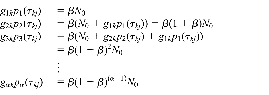
Proof. Suppose that at time slot ${\tau }_{\mathrm{kj}}$ in a time segment $k$ , there are $\alpha$ locomotives transmitting their data simultaneously to the AP. Suppose the power of the received signals satisfies $g_{1k}{p}_1({\tau }_{\mathrm{kj}})<g_{2k}{p}_2({\tau }_{\mathrm{kj}})<\dots <g_{\alpha k}{p}_{\alpha }({\tau }_{\mathrm{kj}})$ , based on the SIC technique and Theorem 2, we must have

$$\begin{array}{l}{g}_{1k}{p}_1({\tau }_{kj})=\beta N_0\\ g_{2k}{p}_2({\tau }_{kj})=\beta (N_0+g_{1k}{p}_1({\tau }_{kj}))=\beta (1+\beta )N_0\\ g_{3k}{p}_3({\tau }_{kj})=\beta (N_0+g_{2k}{p}_2({\tau }_{kj})+g_{1k}{p}_1({\tau }_{kj}))\\ =\beta (1+\beta {)}^2{N}_0\\ ⋮\\ g_{\alpha k}{p}_{\alpha }({\tau }_{kj})=\beta (1+\beta {)}^{(\alpha -1)}{N}_0\end{array}$$

Then, we have $\alpha =1+\underset{(1+\beta )}{\log }(p_{\alpha k}({\tau }_{\mathrm{kj}})g_{\alpha k}/\beta N_0)$ . Since $g_{\alpha k}=min\{|d_{\alpha k}^{-\lambda },1\}\le 1$ and $p_{\alpha k}({\tau }_{\mathrm{kj}})\le P$ , we have $\alpha \le {\alpha }_{max}=1+\underset{(1+\beta )}{\log }(P/\beta N_0)$ . And since the number of locomotives in time segment $k$ is $n_k$ , Theorem 3 is proved.

By Theorem 3, we only need to check subsets with at most ${\alpha }_{max}$ locomotives to obtain all SIC sets. The number of these subsets is $\sum _{i=1}^{{\alpha }_{max}}C(n_k,i)=O((n_k{)}^{{\alpha }_{max}})$ . Then, we have the following SIC-set algorithm:

• Check all subsets with no more than ${\alpha }_{max}$ locomotives to find all SIC sets and transmission powers.

• Solve equation (8) based on identified SIC sets.

The complexity to find all SIC sets and transmission powers is $O((n_k{)}^{{\alpha }_{max}})·O(n_k)=O((n_k{)}^{{\alpha }_{max}+1})$ . For the second step, since the formulated LP has $O((n_k{)}^{{\alpha }_{max}})$ variables, the complexity to solve this LP is $O(((n_k{)}^{{\alpha }_{max}}{)}^3)=O((n_k{)}^{3{\alpha }_{max}})$ . ³⁴ So, the complexity of the SIC-set algorithm is $O((n_k{)}^{{\alpha }_{max}+1})+O((n_k{)}^{3{\alpha }_{max}})=O((n_k{)}^{3{\alpha }_{max}})$ , which is polynomial.

Note that $(n_k{)}^{3{\alpha }_{max}}$ may still be a large number. To further decrease the complexity, we define a concept of maximum SIC set (see Definition 1) and show that we only need to consider solutions with maximum SIC sets.

Definition 1. An SIC set $S$ is a maximum SIC set if for any locomotive $l_i$ which is closer to the AP than all locomotives in $S$ , $S\cup \{l_i\}$ is not an SIC set.

Theorem 4. For a maximum SIC set $S_{\mathrm{ki}}$ and an SIC set $S_{\mathrm{kj}}\subset S_{\mathrm{ki}}$ , we have (1) the data rate from each locomotive in $S_{\mathrm{ki}}-S_{\mathrm{kj}}$ is positive in $S_{\mathrm{ki}}$ ’s time slot and is zero in $S_{\mathrm{kj}}$ ’s time slot; (2) the data rate from each locomotive in $S_{\mathrm{kj}}$ is the same in both $S_{\mathrm{ki}}$ ’s and $S_{\mathrm{kj}}$ ’s time slots.

Proof. Because $S_{\mathrm{ki}}$ is an SIC set, for each locomotive in $S_{\mathrm{ki}}$ , its data rate is positive in $S_{\mathrm{ki}}$ ’s time slot. In particular, for each locomotive in $S_{\mathrm{ki}}-S_{\mathrm{kj}}$ , its data rate is positive. However, such a node has a zero rate in $S_{\mathrm{kj}}$ ’s time slot since it is not in $S_{\mathrm{kj}}$ . Thus, (1) is proved.

By SIC, stronger signals are decoded and canceled before decoding weaker signals. Since locomotives in $S_{\mathrm{ki}}-S_{\mathrm{kj}}$ are closer to the AP than locomotives in $S_{\mathrm{kj}}$ , signals from locomotives in $S_{\mathrm{ki}}-S_{\mathrm{kj}}$ are stronger than signals from locomotives in $S_{\mathrm{kj}}$ . Therefore, in $S_{ki}$ ’s time slot, before signals from locomotives in $S_{\mathrm{kj}}$ are decoded, signals from locomotives in $S_{\mathrm{ki}}-S_{\mathrm{kj}}$ are all canceled. Thus, the decoding process for locomotives in $S_{\mathrm{kj}}$ is the same in both $S_{\mathrm{ki}}$ ’s and $S_{\mathrm{kj}}$ ’s time slots, yielding the same data rates. Hence, (2) is also proved.

Based on Theorem 4, it is easy to see that if we replace $S_{\mathrm{kj}}$ by $S_{\mathrm{ki}}$ in a solution, the new solution will have a better objective value. Thus, we only need to consider maximum SIC sets in equation (8) to obtain an optimal solution. We call this approach as the max-SIC-set algorithm.

We now show how to find all maximum SIC sets (see pseudocode in Figure 3). Initially, we have an empty set and then add locomotives to this set while keeping it as an SIC set. We sort the locomotives by their distances to AP and then try to add locomotives from the farthest one to the closest one. During this process, if we cannot find a locomotive $l_j$ that is closer to AP than any locomotive in an SIC set $S$ such that $S\bigcup _{\{}{l}_j\}$ is an SIC set, then $S$ is a maximum SIC set. Otherwise, $S$ is not a maximum SIC set and we need to further check whether $S\bigcup _{\{}{l}_j\}$ is a maximum SIC set.

Figure 3.

Pseudocode for getting all maximum SIC sets.

The complexity of the algorithm in Figure 3 is not easy to analyze. Instead, we can compare it with the approach of checking all subsets with no more than ${\alpha }_{max}$ locomotives to find all SIC sets. This algorithm has much less complexity due to the following two reasons. (1) We do not check all subsets with no more than ${\alpha }_{max}$ locomotives, that is, once a set is identified as not an SIC set, we will not add more locomotives to this set and check whether the new set is an SIC set or not (since the new set will not be an SIC set). (2) When we check a new set, we only need to determine the transmission power of the newly added locomotives (other locomotives’ powers are already determined) and compare it with $P$ .

In the real environment, the max-SIC-set algorithm will be run on the AP in each beginning of a time segment. To do that, the AP will first get all distances from the covered locomotives, then get all maximum SIC sets using the algorithm shown in Figure 3, and then allocate time slots and transmission powers for these locomotives. After doing this, all locomotives will run using the allocated time slots and the transmission powers during the whole time segment.

Simulation results

In this section, we give simulation results to show the performance of the max-SIC-set algorithm. We compare our results with the other two schemes: SIC only (no power control) and non-SIC (traditional approach). Under these two schemes, each locomotive uses the maximum power to transmit data. Similar algorithms can be designed to obtain optimal solutions under these two schemes.

Consider wireless networks with 20–50 mine locomotives and one AP in a straight tunnel. A locomotive’s maximum transmission power is $P=1\mathrm{W}$ , and the noise power is $N_0={10}^{-10}\mathrm{W}$ . The SINR threshold is $\beta =3$ . The path lost index is $\lambda =4$ . Then, by equation (1), a locomotive’s communication range is $R_{max}=240\mathrm{m}$ . The channel bandwidth is $W=22\mathrm{MHz}$ . The minimum data transmission rate requirement $r_i$ is between 100 kbps and 1 Mbps. The traveling speed is $v=5\mathrm{m}/s$ . The maximum length of a time segment is 5 s. The distance between two successive locomotives should be kept at least 30 m for safety reasons. Suppose we have known all start times $t_i^s$ , which are created randomly in our simulations and satisfy the minimum security distance. The algorithm can be written by any of computer languages, and we use $C\#$ based on VisualStudio.Net 2012 platform. The LP problem can be calculated by some math tool packages, such as LINDO which we select to use. The computer we used has an Intel Core i5 CPU and 4 GB memory. All the following results are obtained in seconds.

We first present detailed results of a wireless network with $20$ locomotives; then, we provide complete results of all network instances with different number of locomotives.

Results of a wireless network with 20 locomotives

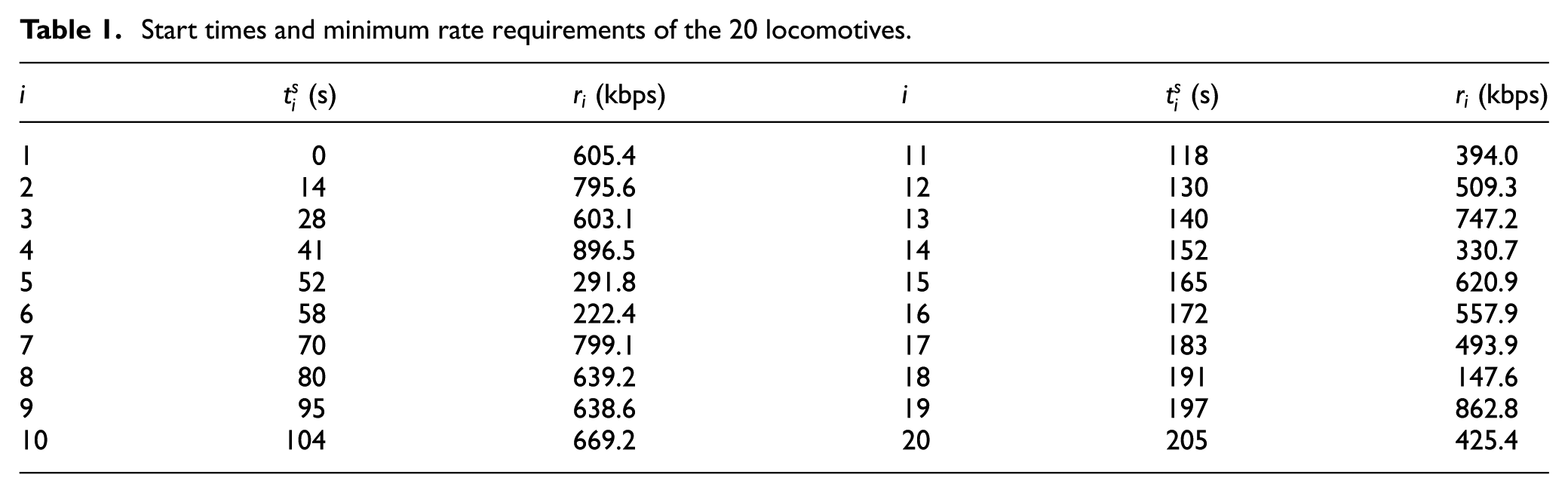
Consider a wireless network with $20$ locomotives. The start times and the minimum data transmission rate requirement of each locomotive are given in Table 1. The whole schedule time $T=301\mathrm{s}$ and will be divided into $79$ time segments. To show the efficiency of our algorithm, we list the values of $K_k$ from the 21st time segment to the 25th time segment (We do not show result in the first $10$ time slots since there are only a few locomotives within AP’s coverage.) in Table 2 while comparing the values of $K_k$ under the other two schemes. We also list the lengths of some time segments in Table 2. We can see that SIC with power control can always achieve the best performance, while the non-SIC scheme always has the worst performance. To show the overall performance over all segments, we calculate the average $K_k$ values for all segments, which are $K=2.71$ for the SIC with power control scheme, $K=2.20$ for the SIC only scheme, and $K=1.80$ for the non-SIC scheme. That is, the improvement in throughput by the SIC with power control scheme is $123.2\%$ compared with the SIC only scheme and is $150.6\%$ compared with the non-SIC scheme.

Table 1.

Start times and minimum rate requirements of the $20$ locomotives.

$i$	$t_i^s$ (s)	$r_i$ (kbps)	$i$	$t_i^s$ (s)	$r_i$ (kbps)
1	0	605.4	11	118	394.0
2	14	795.6	12	130	509.3
3	28	603.1	13	140	747.2
4	41	896.5	14	152	330.7
5	52	291.8	15	165	620.9
6	58	222.4	16	172	557.9
7	70	799.1	17	183	493.9
8	80	639.2	18	191	147.6
9	95	638.6	19	197	862.8
10	104	669.2	20	205	425.4

Table 2.

$K_k$ values under different schemes from $k=21$ to $25$ .

$k$	Time length	$K_k$ (SIC with power control)	$K_k$ (SIC only)	$K_k$ (non-SIC)
21	5	2.29	1.04	0.91
22	5	2.30	1.04	0.91
23	1	1.39	0.91	0.80
24	5	1.88	1.03	0.90
25	3	1.88	1.21	0.90

SIC: successive interference cancellation.

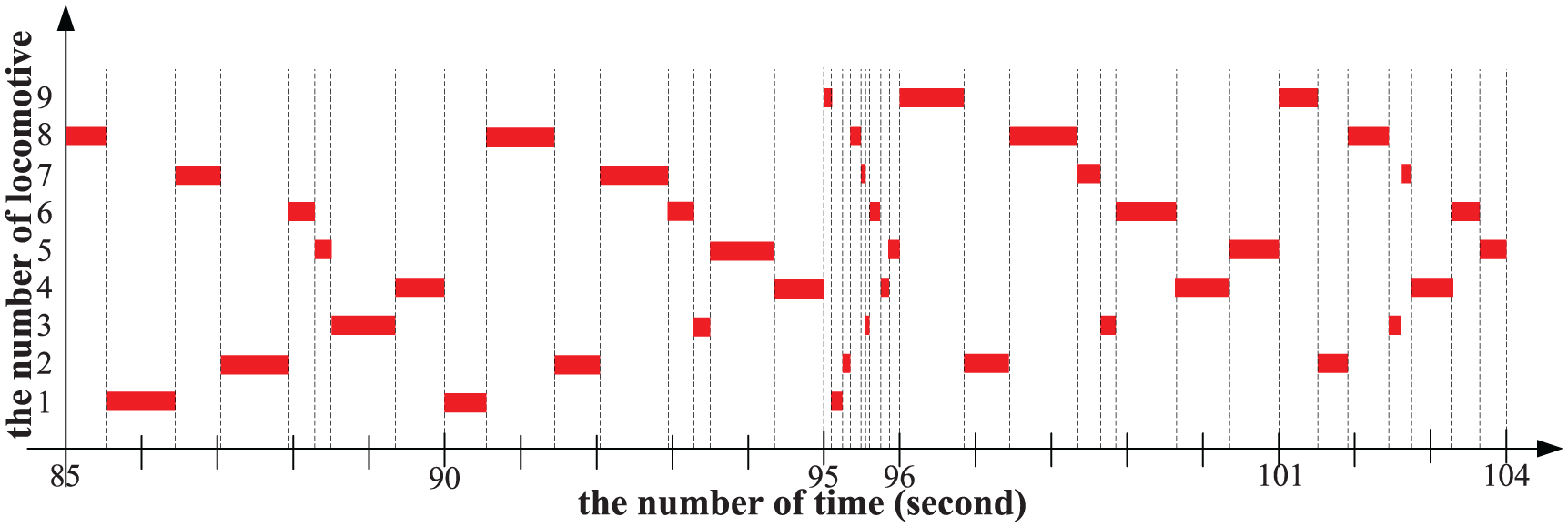
To show the transmission regularity, we draw the locomotives’ transmitting time from the 21st time segment to 25th time segment in Figure 4. From Table 2 and Figure 4, we can see that the length of the 21st segment is 5 s (i.e. the 85th, 86th, 87th, 88th, and 89th second), the length of the 22nd segment is 5 s (i.e. the 90th, 91st, 92nd, 93rd, and 94th second), the length of the 23rd segment is 1 s (i.e. the 95th second), the length of the 24th segment is 5 s (i.e. the 96th, 97th, 98th, 99th, and 100th second), and the length of the 25th segment is 3 s (i.e. the 101st, 102nd, 103rd, and 104th second). So, the total length of these five segments is 19 s. During these 19 s, 9 locomotives are moving along tunnel. In Figure 4, we use the red lines to represent the time slots for each locomotive using. For example, we can see that the first locomotive transmits in the 85th second, 86th second, and a small part of 87th second and that several other locomotives transmit at the same time. For comparison, we draw Figure 5 to show the time segments division under SIC only scheme. Apparently, in this scheme, locomotives have less chances to transmit together. We only find concurrent transmission in five time slots among the total $34$ time slots in these five time segments. We also draw Figure 6 to show the time segments division under non-SIC scheme, and in this scheme, the opportunities for transmitting become worse. Apparently, the locomotives have more opportunities for transmitting under the SIC with power control scheme.

Figure 4.

The locomotives’ transmitting time from the 85th second to the 104th second on the SIC with power control scheme.

Figure 5.

The locomotives’ transmitting time from the 85th second to the 104th second on the SIC only scheme.

Figure 6.

The locomotives’ transmitting time from the 85th second to the 104th second on the non-SIC scheme.

Results of all network instances

We consider networks with $20,30,40$ , or $50$ locomotives and generate $20$ different network instances randomly for each network size. Then, we calculate the $K$ value for each instance under three schemes and show the results in Figure 7. We can see the $K$ value for each instance by the SIC with power control scheme is improved significantly compared with the other two schemes (see Table 3).

Figure 7.

Results of all network instances.

Table 3.

$K$ value and improvements for the four group instances.

Number oflocomotives	$K$ (SIC withpower control)	SIC only		non-SIC
		$K$	Improvement	$K$	Improvement
20	3.25	2.62	123.9%	2.18	148.9%
30	3.47	2.81	123.8%	2.38	145.5%
40	2.68	2.05	130.4%	1.74	153.7%
50	2.59	1.98	131.0%	1.74	148.6%

SIC: successive interference cancellation.

Conclusion

Using SIC technique, an AP can receive multiple locomotives’ data simultaneously. In this article, based on SIC technique and power control, we designed an optimal communication algorithm for underground mine locomotive networks. We divided the whole scheduling time into many time segments and in each time segment, we got an LP formulation for our problem. Then, we designed an algorithm named max-SIC-set algorithm to solve the problem in polynomial time. Simulation results showed that our algorithm can improve the throughput significantly compared with the other two schemes: SIC only (without power control) and non-SIC (traditional approach).