Sage Journals: Discover world-class research

Abstract

This research develops a multi-layer hybrid soft-sensor model to improve the accuracy of building thermal load prediction using integrated data. The multi-layer hybrid model (autoregressive and particle swarm optimization neural network) hybridizes an autoregressive model with exogenous inputs and a particle swarm optimization neural network. The distributed sensors’ experimental scenario was set in a medium-sized office building located in Shanghai, which has applied this multi-layer hybrid model to evaluate the prediction accuracy, meanwhile its performance was also compared with several commonly used methods under different evaluation criteria. Through frequency-domain decomposition, the heat balance equation is used to validate the autoregressive and particle swarm optimization neural network model. Both the simulation of building thermal load and experiment results demonstrate that the proposed autoregressive and particle swarm optimization neural network method can recognize soft sensing of the building thermal load much more quickly and efficiently, and achieve higher accuracy in both cooling load and heating load prediction.

Keywords

Autoregressive model with exogenous inputs particle swarm optimization neural network multi-layer hybrid model (autoregressive and particle swarm optimization neural network)soft sensor thermal load

Introduction

With the rapid worldwide urbanization progress, building load forecasting has received much attention from both academic researchers and governments.^1–3 There has been much research on climate change and comfort standards, among which Kwok and Rajkovich⁴ showed that the building sector thermal load accounted for 38.92% of the total primary energy requirements (PER) of the United States, of which 34.9% was used for building energy consumption. In China, building sector thermal load accounted for approximately 24.11% of national energy use in 1996, rising to 27.52% in 2001, and is estimated to increase to approximately 35.12% in 2020.^5,6 Although carbon emissions per capita in China are lower than those in other developing countries, its total emissions are the second only to the United States. From the previous researches,^7,8 buildings’ energy consumption account for a significant proportion of carbon emissions. It is a statistical fact that the building sector uses approximately 40% of the world’s electricity supply for service system working,⁹ especially in developing countries, such as China. The increasing complexity of building designs and higher performance requirements for achieving sustainability, predicting the load of heating, ventilating, and air-conditioning (HVAC) systems are important for energy management.

There are many forecasting techniques used in load engineering.^10,11 The software developed quickly in the last couple of years to predict building energy consumption, including DOE-2,¹² ESP-r,¹³ EnergyPlus,¹⁴ and DeST.¹⁵ Although different kinds of simulation software can accurately predict the building thermal load in many projects,^16–18 the simulation results differ in the prediction of occupied buildings’ energy consumption.¹⁹ Because of various parameters setting, the building energy simulation software is too complicated and time-consuming. Some of the more popular of the current building energy simulation software are also difficult to identify the influential variables of building thermal load.²⁰ Therefore, the research and establishment of a reasonable and effective building load forecasting model that combines indoor/outdoor information and building characteristics has become an important issue to be addressed.

Soft-sensor techniques are widely used in engineering for measuring the complex parameters. Selection of the appropriate input variables for soft sensor has many potential benefits including eliminating data redundancy, reducing computing time, and predicting with higher accuracy. Various techniques are used to select influential variables for soft sensors which fall under three groups: wrapper methods, filter methods, and embedded methods. The main influential variables, for example, relative compactness,²¹ building location climate,²² surface area, roof area, wall area,²³ and window orientation,²⁴ should be divided into two aspects: the physical materials of buildings and local meteorological conditions; furthermore, the physical materials can be represented by thermal inertia, which is reflected in the historical thermal loads. These factors make the relationship between Environmental Protection Board (EPB) and its influential variables quite complicated. Thus, accurately predicting the heating load (HL) and cooling load (CL) of buildings can be a big challenge.

Plenty of techniques have been used to model building thermal load forecasting. In Yu et al.,¹⁹ classification and regression tree (CART) achieved accurate predictions of building energy requirement with fewer errors. Li et al.²⁵ combined genetic algorithm with adaptive network–based fuzzy inference system to improve accuracy in predicting building energy consumption. Tsanas and Xifara²⁰ applied random forest (RF) technique to predict thermal load in residential buildings. Other proposed hybrid forecasting techniques for identifying and forecasting system behavior include general regression neural network (NN),²⁶ multi-layer NN system,²⁷“Regression-Markov” integration model,²⁸ ensemble approach (support vector regression (SVR) + artificial neural network (ANN)),²⁹ generalized locally weighted group method,³⁰ and hybrid system.²⁶

In summary, they can be classified as traditional methods based on time-series modeling and artificial machine-learning techniques,^{19,20,25–28} and hybrid models of the traditional methods have also achieved effective performances.^25,29,30 However, load forecasting is characterized with stochastic properties and strong non-linearity. Therefore, a new hybrid model proposed here is supposed to possess a high-level ability to handle the various problems mentioned above.

The above studies underpin the satisfactory performance of the hybrid model in forecasting energy consumption in different kinds of buildings. However, the prediction performance of the aforementioned studies shows that hybrid soft-sensor techniques still needs further study, which makes this research more meaningful to fill this gap using these models individually and in combination with predicting thermal load via soft-sensor measurement validation and multiple performance measures.

Building thermal load prediction is characterized with stochastic properties and strong non-linearity. It is a complex procedure for the formation of the building thermal load, which is composed of indoor heating influence and outdoor weather condition impact. Therefore, this article proposed to use autoregressive model with exogenous inputs (ARX) to handle the problem of thermal inertia, for its dynamic nature can solve time delay of heat conduct well. Also, particle swarm optimization neural network (PNN) is used to overcome nonlinear and strong coupling features of the heating system in a wide range. The main results and contributions are described as follows:

The first contribution of this article is the building of a multi-layer hybrid model (autoregressive and particle swarm optimization neural network (APNN))—a combination of dynamic liner model (ARX) and static nonlinear model (PNN). Therefore, the APNN can be regarded as a dynamic nonlinear model which is well suited for processing thermal load prediction.

Computational fluid dynamics (CFD) software FLUENT is then used to simulate the temperature distribution of the experimental room, and the simulation results are compared to sensor measurements to obtain the building reference temperature.

Through frequency-domain decomposition, a real-time soft-sensing technology utilizing the room heat balance equation is employed to validate the APNN model with actual measurement data.

This article finally compares the performance of APNN with other popular predicting methods through lots of experiments, among which the experimental data include not only simulation but also practical measure.

Multi-layer hybrid model structure and research challenges

The goal of this research is to establish a hybrid thermal load prediction model and validate the model accuracy via simulations and real experiments. This article is divided into three main parts: (1) first, the multi-layer hybrid thermal load forecasting model (APNN) is proposed, namely, the ARX and PNN, which combines the advantages of information-integrated autoregressive (AR) model and PNN by prediction error (PE); (2) CFD software FLUENT is then used to simulate the temperature distribution of the experimental room, and the simulation results are compared to sensor measurements to obtain the building reference temperature; (3) through frequency-domain decomposition, a real-time soft-sensing technology utilizing the room heat balance equation is employed to validate the APNN model with actual measurement data. An overview of the research structure is shown in Figure 1. Based on the whole research process, the obtained solutions are shown in Table 1.

Figure 1.

Overview of the research process.

Table 1.

Obtained solutions for the challenges in this research.

	Challenges	Proposed solutions
1	Integrated building thermal load influence factors	Simulation and actual measurement
2	Input selection	Correlation function
3	Normalization	Mix–max normalization
4	Time-series analysis model optimization	ARX
5	Artificial intelligence model optimization	PNN
6	Multi-layer hybrid model	Combination of ARX and PNN
7	Building thermal load un-measurable	Frequency domain decomposition
8	Reference temperature	32-point temperature sensors
9	Validation	Heat balance equation
10	Evaluation criteria	MAPE, RMSE and MAE

ARX: autoregressive model with exogenous inputs; PNN: particle swarm optimization neural network; MAPE: mean absolute percentage error; RMSE: root mean squared error; MAE: mean absolute error.

Model structure and optimization

Building thermal load formation analysis

Building thermal load is composed of indoor heating influence and outdoor weather condition impact; each section operates under a different mechanism, but has a great influence on building thermal load.

Indoor load mainly originates from electrical work and body heat radiation, among others. It can be predicted by simplified calculations following the laws of heat dissipation. The outdoor environment building load influence index includes temperature, solar radiation, and humidity. The whole building load is generated under the combined action of indoor and outdoor influences. In our previous research,³¹ we constructed different types of models based on the indoor/outdoor information mentioned previously. The ARX was proposed for building load forecasting with the combination of multiple linear regressions (MLR) of meteorological data and AR modeling using historical data as inputs. The structures of three types of thermal load prediction models are shown as Figure 2.

Figure 2.

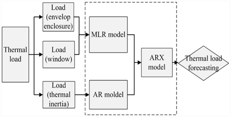
Structure of three types of thermal load prediction models.

The ARX model order optimization

A time series can be used as a resource of knowledge acquisition and a method for forecasting the future. In the evaluation process, analysis is important to examine the degradation of trends, seasonal growth, and cyclical fluctuations. The selection of the method used for forecasting future values depends on the purpose of the estimation, type, and elements of the time series, amount of data, and length of the estimation period.

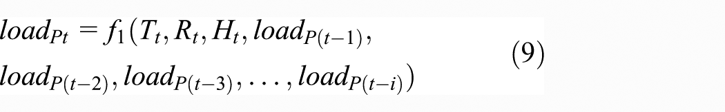
The Box–Jenkins method is the most widely used model for time series modeling, which includes an ARX, and it has previously been used in load forecasting. Taking into account the thermal storage of building space, the influence of external meteorological factors and historical thermal factors will be stored in a certain form of building materials because of thermal inertia. Naturally, thermal inertia will impact the thermal load at the current moment. When using an hourly time interval, the key to the ARX model is to determine the optimal order to ensure prediction accuracy. According to our previous research,³¹ the formulation of the ARX model is conducted as follows

\begin{matrix} Loa d_{t} = & W_{1} T + W_{2} R + W_{3} H + W_{4} loa d_{t - 1} \\ + W_{5} loa d_{t - 2} + W_{6} loa d_{t - 3} + \dots + W_{9} loa d_{t - 6} + e \end{matrix}

(1)

where the load_t is the prediction result, T is the outdoor temperature, H is the humidity, R is the solar radiation, $w_{t - i}$ is the ith order of the AR parameters, $loa d_{t - i}$ is the ith load prediction result, and e is the white noise.

According to function (1), continuous study of the ith order of the ARX model (i = 1–7) is required to achieve the minimum error value based on data of 1 week in July. Figure 3 and Table 2 compare the absolute error with the simulation data.

Figure 3.

First- to seventh-order ARX model absolute error curve.

Table 2.

First- to seventh-order ARX model absolute error value.

Model order	i = 1	i = 2	i = 3	i = 4	i = 5	i = 6	i = 7
AE	−1.1	−0.8	−0. 8	−0.7	−0.8	−0.7	−0.8
	−0.5	−0.4	−0.3	−0.3	−0.3	−0.2	−0.4
	…	…	…	…	…	…	…
	1.2	1.2	1.0	1.4	1.3	1.0	1.3
	2.2	.2.8	3.2	3.3	3.1	0.6	0.8
MAE	1.79	1.68	1.65	1.66	1.75	1.49	1.52

ARX: autoregressive model with exogenous inputs; AE: absolute error; MAE: mean absolute error.

It can be clearly observed that the absolute error will be a minimum value when the ARX model is a sixth-order (i = 6) model.

The PNN

ANN has been verified as a universal intelligent method and has been widely applied in engineering studies. The most widely used and effective NN model is the back-propagation neural network (BPNN).^{19,20,25–27,29} Activation of each neuron in a hidden output layer is computed as equation (2)

ne t_{k} = \sum w_{kj} o_{j} and y_{k} = f (ne t_{k}) = \frac{1}{1 + e^{- ne t_{k}}}

(2)

In the above equation, $ne t_{k}$ is the activation of the kth neuron, j is the set of neurons in the preceding layer, $w_{kj}$ is the connection weight between neuron k and neuron j, O_j is the output of neuron j, and y_k is the sigmoid or logistic transfer function.

Particle swarm optimization (PSO) is a bio-inspired global optimization technique that was proposed by J Kennedy and R Eberhart.³² PSO performs a population-based search, using particles to represent potential solutions within the search space. Each particle is characterized by its position, velocity, and a record of its previous performance. At each flight cycle (iteration), each particle’s velocity and position is formulated as

\begin{array}{l} v_{j} (n + 1) = ω \cdot v_{j} (n) + c_{1} r_{1} (p_{j} (n) \\ - x_{j} (n)) + c_{2} r_{2} (p_{g} (n) - x_{j} (n)) \end{array}

(3)

x_{j} (n + 1) = v_{j} (n + 1) + x_{j} (n)

(4)

where $v_{j} (n)$ is the speed of the jth particle in the nth generation, r₁ and r₂ are the random numbers following a uniform distribution in the range of [0, 1], c₁ and c₂ are the constants named acceleration coefficients, $x_{j} (n)$ is the position of the jth particle in the nth generation, $p_{j} (n)$ is the best position yielding the best fitness value for the jth particle, $p_{g} (n)$ is the best position discovered by the whole particles, and w is the weight used to balance the global and local search abilities.

PSO method has several advantages for exploring the hyperspace global optimum, especially the fast convergence. In order to improve its capability of global search and avoid local minimization, the genetic operations including crossover and mutation are further introduced to update method of PSO algorithm. The improved PSO algorithm is proposed by Li et al.³³ The crossover and mutation equations are the essential part of the algorithm, which are described as follows:

Crossover equations

{\begin{matrix} chil d_{1} (X_{i}) = p_{i} * paren t_{1} (X_{i}) + (1 - p_{i}) * paren t_{2} (X_{i}) \\ chil d_{2} (X_{i}) = p_{i} * paren t_{2} (X_{i}) + (1 - p_{i}) * paren t_{1} (X_{i}) \end{matrix}

(5)

{\begin{matrix} chil d_{1} (V_{i}) = \frac{paren t_{1} (V_{i}) + paren t_{2} (V_{i})}{| paren t_{1} (V_{i}) + paren t_{2} (V_{i}) |} * | paren t_{1} (V_{i}) | \\ chil d_{2} (V_{i}) = \frac{paren t_{1} (V_{i}) + paren t_{2} (V_{i})}{| paren t_{1} (V_{i}) + paren t_{2} (V_{i}) |} * | paren t_{2} (V_{i}) | \end{matrix}

(6)

Mutation equation

x'_{i} = x_{i} + rand * N (0, 1)

(7)

where p_i is a uniformly distributed random value between 0 and 1; parent_j(X_i) and parent_j(V_i) represent the position and velocity of parental particle, respectively; and child_j(X_i) and child_j(V_i) stand for the position and velocity of offspring, respectively (j = 1, 2).

To mitigate the drawbacks and incorporate the advantages of NN and PSO, the combination of an NN and particle swarm optimization artificial intelligent model, named PNN, is used in this research. Figure 4 illustrates a basic PNN feedforward network topology structure.

Figure 4.

Structure of a basic PNN network.

The proposed multi-layer hybrid model (APNN)

As indicated above, the multi-layer hybrid model (APNN) is proposed through the following steps:

The integrated load factors include meteorological data and historical data acquired by sensor measurements and the DeST software.

Modeling an ARX by least-squares support vector machine (LS-SVM) identification. Then, evaluate the “error” value gained by comparison of the thermal loads generated by the DeST and ARX model; the “error” value and meteorological data become a new set of inputs in PNN for training the data to obtain the PE.

Finally, the sums of forecasting thermal load and PE are calculated using the ARX model and PNN, respectively, and are the final results of the hybrid model.

The structure of the hybrid model is shown in Figure 5. The features of this methodology are as follows. (1) Because some existing techniques can model different types of building information separately, all of the information, including the historical thermal load and meteorological information, can be utilized for one integrated technique. (2) Integrating all of the information can help improve the prediction accuracy, as well as extend the prediction coverage. (3) The proposed hybrid model APNN can allow traditional NN to incorporate both types of uncertainties of inputs and network parameters to better handle the uncertainties of load forecasting compared to other relevant methods.

Figure 5.

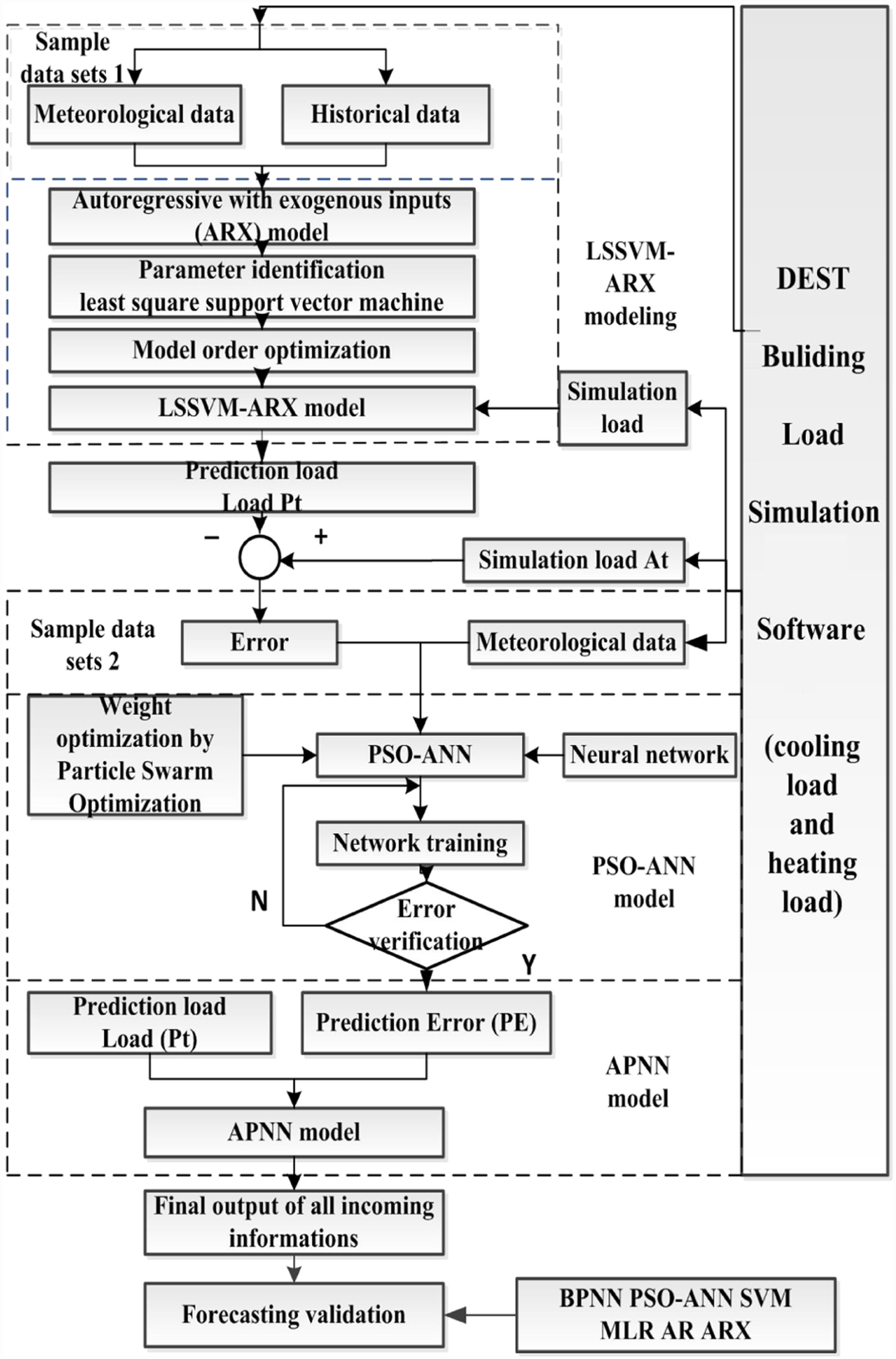
Design schematic of the hybrid model.

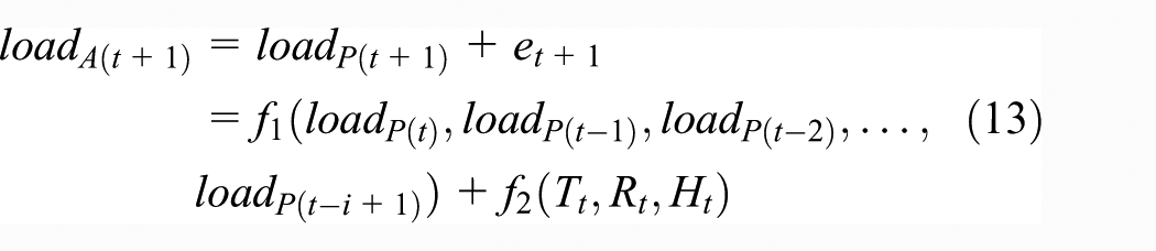
In this research, a hybrid model is proposed so that all of the information, including the historical load data predicted by a time-series model and meteorological information used in the artificial intelligent model can be utilized for modeling; we consider that the actual value $loa d_{At}$ can be expressed as a set of predictive value $loa d_{Pt}$ plus a PE term $e_{Pt}$

loa d_{At} = loa d_{Pt} + e_{t}

(8)

First, the historical information is used to explore the historical information load p_(t−i)

\begin{array}{l} l o a d_{P t} = f_{1} (T_{t}, R_{t}, H_{t}, l o a d_{P (t - 1)}, \\ l o a d_{P (t - 2)}, l o a d_{P (t - 3)}, \dots, l o a d_{P (t - i)}) \end{array}

(9)

Once load_Pt is available, the error terms actually are the difference between the actual values and predictions, that is

e_{t} = loa d_{At} - loa d_{Pt}

(10)

Here, this research assumes that the PE term e_t is caused by past conditions of factors, and by employing the PNN model to describe the relationship between them, the error term can be defined as

e_{t} = f_{2} (T_{t - 1}, R_{t - 1}, H_{t - 1})

(11)

where f is a nonlinear function determined by PNN and T_t−₁, and R_t−₁ and H_t−₁ are the meteorological parameters of temperature, solar radiation and humidity at time t−1, respectively. After sufficient training and learning, the trained PNN can be used to forecast the future PE, e_t + 1

e_{t + 1} = f_{2} (T_{t}, R_{t}, H_{t})

(12)

Because the future prediction load_P_(t + 1) can be forecasted by the ARX model, the final result is the combination of load_P_(t + 1) and e_t_+ 1

\begin{matrix} loa d_{A (t + 1)} & = loa d_{P (t + 1)} + e_{t + 1} \\ = f_{1} (loa d_{P (t)}, loa d_{P (t - 1)}, loa d_{P (t - 2)}, \dots, \\ loa d_{P (t - i + 1)}) + f_{2} (T_{t}, R_{t}, H_{t}) \end{matrix}

(13)

Soft-sensing technology based on time-frequency decomposition

Soft sensors are predictive mathematical models that infer the values of a given process variable from measurements of other variables.^34,35 Because the room thermal load cannot be measured directly, the parameter identification for the soft-sensing model cannot be realized with the sample data. If this bottleneck cannot be solved, room CL soft sensing is difficult to realize. According to our previous research,³⁶ the frequency-domain decomposition based on some assumptions for engineering calculations was used to realize the room thermal load soft sensing.

Room heat balance equation

The heat balance equation in the room system is as follows

Load (n) = HE (n) - HS (n)

(14)

where $Load (n)$ is the hourly room CL, $HE (n)$ is the hourly heat extraction (HE) of the air-conditioning system, and $HS (n)$ is the hourly heat storage in the room system. If the HE and heat storage can be obtained, the room CL can be calculated with equation (14).

The room air temperature is changed by air-conditioning recursively delivering low-/high-temperature air to the room system. The energy variation of air-conditioning operation is defined as HE, which can be calculated with the enthalpy difference as follows

HE (n) = G (c_{p . g} + c_{p . q} φ d_{b}) (T_{out} - T_{in})

(15)

where G is the air mass flow (kg/s), $c_{p . g}$ is the dry air heat capacity at constant pressure, $c_{p . q}$ is the water vapor heat capacity at constant pressure, $φ$ is relative humidity, $d_{b}$ is the saturation humidity ratio, $T_{out}$ is the outlet air temperature, and $T_{in}$ is the inlet air temperature.

The difference between the actual HE rate and the thermal load (equation (14)), in practice, is caused by either the variation of the air temperature from the reference value used to calculate the thermal load or the HVAC system characteristics (equation (15)).³⁷ The current hourly heat storage is defined as the difference in the rate of HE and room CL at the current hour. Heat storage in the building space is dependent on the grid architecture. The relationship between heat storage and room air temperature can be written as follows

HS (n) = \sum_{i = 0}^{\infty} {k_{i}}^{*} Δ T

(16)

where $Δ T$ is the deviation of air temperature from the reference value i, $Δ T = T_{a} - T_{s}$ , where $T_{a}$ is the current room reference temperature and $T_{s}$ is the air-condition set temperature; and $k_{i}$ is the corresponding heat storage coefficient of the ith model order.

HE can be calculated via equation (15), and heat storage can be described by the room air temperature response equation of equation (16). If the corresponding heat storage coefficient can be obtained, according to equations (15) and (16), the room thermal load soft sensing can be realized as follows

Load (n) = HE (n) - \sum_{i = 0}^{\infty} {k_{i}}^{*} Δ T

(17)

In fact, an infinite order time series obviously has no maneuverability. In view of this, the truncation operation is employed in soft sensing for room thermal load as follows

Loa d_{n} = H E_{n} - \sum_{i = 1}^{k} {k_{i}}^{*} Δ T_{n - i}

(18)

The mechanism of the room thermal load is analyzed, and so are the simulation data from the building energy consumption simulation tool kits. It is found that in the frequency domain, the room thermal load distribution is concentrated on the frequency point with a period of 1 day and its second and third harmonics.

Through frequency-domain decomposition, the parameters of the soft-sensing model in the heat storage process were identified in the frequency range without thermal load, so the method avoids the dependence on the real value of the un-measurable room thermal load.

According to the employment of fast Fourier transform (FFT), the heat balance equation (18) in the frequency domain is re-written as

\begin{matrix} Load (w) = HE (w) - \sum_{i = 1}^{k} k_{i} Δ T (w) e^{- jwi}, w = w_{1}, w_{2}, w_{3} \\ 0 = HE (w) - \sum_{i = 1}^{k} k_{i} Δ T (w) e^{- jwi}, w \neq w_{1}, w_{2}, w_{3} \end{matrix}

(19)

Thus, the hourly room thermal load can be separated from the sample data containing the time series of HE and room air temperature. To realize the soft sensing of the room CL at all times, the heat storage coefficient in equation (19) needs to be identified. With the known heat and extraction, room thermal load and room air temperature, the heat storage coefficient can be obtained according to the least-squares method, and the soft sensing for the room thermal load can be realized using equation (18).

Room reference temperature

As indicated in previous studies, it is expected that the building thermal load results will be significantly impacted by the choice of an appropriate reference air temperature for the calculation of the room thermal load.

This means that the air temperature distribution needs to be considered for indoor environments when calculating the differential temperature $Δ T$ in the heat balance equations (18) and (19).

To obtain an accurate reference room temperature, a case study of a single office room with a floor air-conditioner was conducted. The room has dimensions of 7.7 m × 4.4 m × 3.6 m for length, width and height, respectively. Air is injected into the room with an incoming velocity of 2.15 m/s from the rectangular inlet of the air-conditioner (235 mm × 495 mm) and leaves the room via the air-conditioner outlet (610 mm × 495 mm). In the experimental setting, the air-conditioning is set to operate for 1 h per test. The two-dimensional and three-dimensional room structures are shown in Figure 6.

Figure 6.

Room structure.

There are 32 points representing the 32 locations as shown in Figure 7. Among them, the six black points are distributed on the backs of two chairs, the seats of two chairs, the center of the table, and the outlet of the air-conditioner; the white points are distributed on the window, door, window on the door, inlet of the air-conditioner, south wall, west wall, and floor; and the gray points are distributed on the ceiling, north wall, east wall, and cabinet. There is also an isolated white point outside the room that is used to collect the outdoor temperature as the operating condition.

Figure 7.

Temperature sensor arrangement plan in the room.

In this experiment, with a combination of hardware and software, simultaneous multiple-point temperature measurements were obtained, collected, sorted, and saved with 32 PT100^38,39 temperature sensors applied in the room, and the 4–20 mA current signals, which were output from the temperature transmitters, were converted to 1–5 V analog voltage signals. Analog voltage signals were connected to the PISO-813 card, which was embedded in an industrial personal computer (IPC). The software received the 32 signals from the hardware mainly for data processing, display, storage, and querying. It also includes the data conversion interface, through which data can be saved in Excel files. The data were collected every 10 s.

In the supplemental materials, the temperature automatic monitoring system is shown in Figures 1 and 2. The inlet and outlet of air-condition temperature monitoring situation are shown in Figure 3. The details about temperature sensor locations are shown in Table 2.

The multi-layer hybrid model case study and results validation

Data sources

To verify the authenticity and universality of the model, data sources are divided into two types of measurements and simulations.

The integrated building simulation software DeST was employed because it is widely used in civil and commercial building applications. DeST⁴⁰ building simulation software involves the integration of the building environment and its air-conditioner control system. DeST can be used as a building environment and its control system simulation platform due to its advantages of flexibility and the openness and high scalability of the calculation module.

Building exterior meteorological data were obtained from the TBS-YG5 meteorological monitoring station in the form of real-time integrated temperature, humidity, and total solar radiation. The details of the data sources can be seen in Figure 8.

Figure 8.

Data source schematic diagram.

In the supplemental materials, the experiment field of TBS-YG5 meteorological monitoring station working during daytime and night time is shown Figures 4 and 5.

Case study

A medium-sized office building in a Shanghai academic institute has applied for this experiment. The building exterior and interior structures are shown in Figures 9 and 10, respectively. The simulation result sample data are shown in Table 1 in the supplemental materials. The whole sample year meteorological data trend is shown in Figure 11.

Figure 9.

Building exterior structure.

Figure 10.

Building interior structure.

Figure 11.

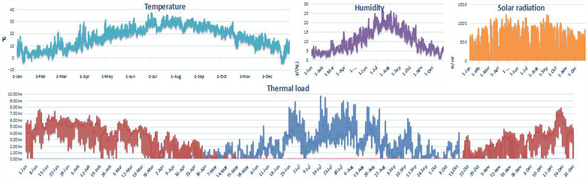
Meteorological data trend of the whole sample year.

Through DeST software simulation, we can obtain typical annual weather data for a total of 8760 h. From the load trend curve, it can be observed that the maximum HL occurs in January and the maximum CL occurs in July. For this reason, we select 2 months (January and July) of data as input to the hybrid model proposed above to study the building thermal load.

The proposed multi-layer hybrid model is introduced and concluded as the best-fit model for forecasting the building load value of Shanghai city. To reinforce this conclusion, several popular prediction methods are examined for comparison.

Evaluation criteria

In this research, the root mean squared error (RMSE), mean absolute error (MAE), and mean absolute percentage error (MAPE) are computed to verify the models’ performance. The equations are as follows

RMSE = \sqrt{\frac{1}{N} \sum_{t = 1}^{N} {| a_{i} - p_{i} |}^{2}}

(20)

MAE = (\frac{1}{n}) \times \sum_{t = 1}^{N} (| a_{i} - p_{i} |)

(21)

MAPE = \frac{1}{N} \sum_{t = 1}^{N} (\frac{| a_{i} - p_{i} |}{a_{i}}) \times 100

(22)

where a_i and p_i are the actual and prediction values of building load (cooling or heating) of ith hour, respectively, and N is the number of testing hours. The data from July and January were used for predicting cooling and HL, respectively. The experiment results are shown in Figures 12 and 13 and Table 3.

Figure 12.

Absolute error trend of the cooling load in July according to the different methods.

Figure 13.

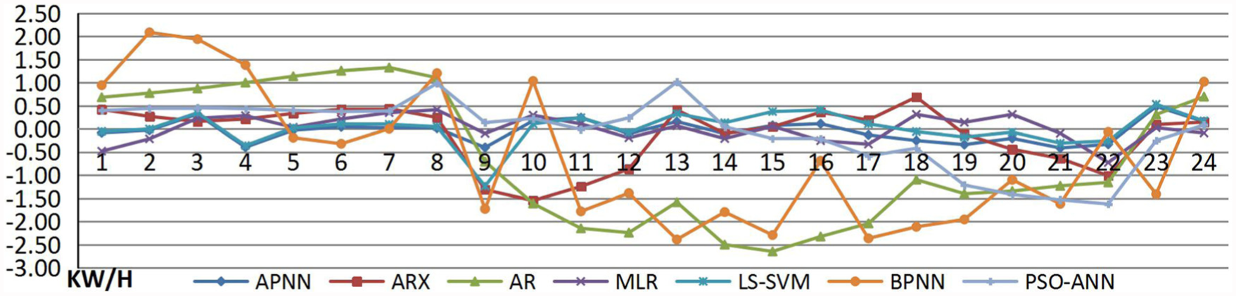
Absolute error trend of the heating load in January according to the different methods.

Table 3.

Performance examination for different prediction methods.

Model	Cooling load (July)					Heating load (January)
Model	MAPE (%)	RMSE (kw)	MAE (kw)	Maximum error (kw)	Minimum error (kw)	MAPE (%)	RMSE (kw)	MAE (kw)	Maximum error (kw)	Minimum error (kw)
PNN	14.899	1.058	0.829	2.513	−0.681	16.323	0.721	0.546	1.014	−1.622
BPNN	23.013	1.622	1.284	3.568	−2.393	46.394	1.542	1.368	2.085	−2.390
LS-SVM	7.988	0.613	0.450	1.775	−0.797	7.531	0.344	0.234	0.531	−1.237
MLR	19.481	1.393	1.115	3.835	−1.105	15.938	0.638	0.488	0.689	−1.551
AR	31.036	2.454	1.949	5.297	−0.496	50.306	1.517	1.384	1.325	−2.649
ARX	15.012	1.019	0.819	2.215	−0.865	6.916	0.280	0.231	0.414	−0.728
APNN	7.654	0.540	0.411	1.420	−0.759	5.877	0.238	0.192	0.486	−0.412
Mean	17.012	1.243	0.983	2.946	−1.014	21.326	0.754	0.635	0.935	−1.513

MAPE: mean absolute percentage error; RMSE: root mean squared error; MAE: mean absolute error; PNN: particle swarm optimization neural network; BPNN: back-propagation neural network; LS-SVM: least-squares support vector machine; MLR: multiple linear regressions; AR: autoregressive; ARX: autoregressive model with exogenous inputs; APNN: autoregressive and particle swarm optimization neural network.

For each single model, computing efficiency is another critical factor that should be evaluated during model development. Table 5 shows the computing time in predicting CL and HL and the computer specifications.

Results analysis

The absolute error trend curves in Figures 12 and 13 clearly show that the proposed hybrid model (APNN) that hybridizes ARX and PNN has higher accuracy than other popular methods, including the time-series models (AR, MLR, and ARX) and artificial intelligence methods (LS-SVM, ANN, and PNN).

Table 3 shows the performance results for the prediction models, including the PNN, BPNN, LS-SVM, MLR, AR, ARX, and hybrid APNN models. The accuracy measures were used to evaluate the predictive techniques.

Table 3 describes the analytical results for each single and ensemble models. The statistical index (MAPE, RMSE, and MAE) shows that the accuracy of the ARX model results of 15.012%, 1.019, and 0.819 (July, CL) and 6.916%, 0.280, and 0.231 (January, HL), respectively, are superior to the other time-series models; meanwhile, the accuracy of the PNN model results of 14.899%, 1.058, and 0.829 (July, CL),and 16.323%, 0.721, and 0.546 (January, HL), respectively, are superior to the other machine-learning methods.

In particular, the accuracy of the results of the hybrid APNN model hybridized with ARX and PNN of 7.654%, 0.54, and 0.411 (July, CL) and 5.877%, 0.238, and 0.192 (January, HL), respectively, had an even better overall performance compared to all of the other models with regard to building load forecasting.

Based on the numerical evaluation, Figures 14 and 15 further show that the performance measures (RMSE, MAE, and MAPE) of the experiment models identified in Table 3 are superior to those of the models reported in the literature. In the CL and HL phases, the APNN model had a higher prediction accuracy compared to the other individual models and those reported in the literature.

Figure 14.

Criteria for evaluating comparative models of the cooling load.

Figure 15.

Criteria for evaluating comparative models of the heating load.

Results validation

As is mentioned above, this article uses actual measured data of a winter day to validate the proposed hybrid model via two methods: (1) a typical 24-h day in winter was selected for study; building exterior meteorological data obtained from the TBS-YG5 meteorological monitoring station are shown in Table 3 in the supplemental materials; these measured meteorological data were input into the DeST building simulation to obtain the current building thermal load; (2) from the frequency-domain characteristics of the heating balance equation (14), a real-time soft-sensing technology for room thermal load is used based on room temperature response frequency-domain characteristics to validate the proposed hybrid APNN model.

The distribution of the thermal environment under air-conditioning is shown in Figure 16 and can be described by Tecplot360. According to the actual temperature measurement, Table 4 lists several temperature values of the heating balance equation (19).

Figure 16.

Distribution of thermal environment of the experimental day.

Table 4.

Parameter value.

	Location	Typical day measured temperature per hour (°C)			Mean
T _a (°C)	Table	19.53	…	19.41	20.5
	Chair A	19.36	…	18.82
	Chair B	19.76	…	19.67
	Chair C	21.05	…	20.70
	Chair D	22.90	…	22.38
T _s (°C)	25
T _in (°C)		38.06	…	39.21	41
T _out (°C)		20.01	…	21.33	29.8
HE (KW/h)	12.5

The reference temperature $T_{a}$ can be obtained from the average value over 24 h of the temperature sensors, as shown in Figure 7. The set temperature of the air-conditioning system $T_{s}$ is 25°C, which meets the requirements of indoor temperature thermal comfort $T_{in}$ (°C) and $T_{out}$ (°C), are the average temperatures of the air-conditioner inlet and outlet, respectively, measured over 24 h. HE is calculated by equation (15). The computational results of the different verification methods mentioned above are shown in Figure 17.

Figure 17.

Computational results of the different verification methods.

The red curve in Figure 17 demonstrates that the proposed hybrid APNN model can fit well to the DeST input data and the FFT heat balance equation computational results, respectively. The maximum, minimum, and average relative errors (REs; purple curve) between the APNN model and the FFT heat balance equation computational results, which can be regarded as the reference thermal load, respectively, are −17.33%, 1.09%, and 9.07%, respectively; furthermore, the yellow trend line shows that RE is below ±5%. Although this experiment uses actual data and high precision as simulation results, in a real-life scenario, considering clouds, shadows, and weekday versus weekend occupancy, such a result would also be acceptable.

In practice, the evaluation of the proposed hybrid model computing efficiency should take both prediction accuracy and computing speed into consideration. For each individual method, Table 5 shows the computing speed in forecasting the thermal load, as well as the computer’s performance. The computational data show that the proposed APNN model can predict the thermal load within seconds. Therefore, it has the features of real-time processing that provides a good solution for complex and changeable weather and climate.

Table 5.

Computing efficiency.

Model	Average time (s)		Hardware specification and software adopted
Model	CL	HL
PNN	1.40	1.50	CPU: Intel Pentium G2030 at 3 GHz
BPNN	1.60	1.80	RAM: 2 GB
LS-SVM	3.91	4.11	System type: 32-bit Operating System
MLR	0.58	0.58
AR	0.58	0.59
ARX	1.60	1.61
APNN	2.80	3.00
FFT	8
DeST	2400

PNN: particle swarm optimization neural network; BPNN: back-propagation neural network; LS-SVM: least-squares support vector machine; MLR: multiple linear regressions; AR: autoregressive; ARX: autoregressive model with exogenous inputs; APNN: autoregressive and particle swarm optimization neural network; FFT: fast Fourier transform.

Conclusion

Various real-time prediction modeling techniques, including ANN, PNN, LS-SVM, MLR, AR, ARX, and the proposed hybrid model (APNN), were compared in terms of performance indicators and computing speed in predicting thermal load of experimental building. The proposed hybrid model (APNN) is easily performed and can quickly respond. The meteorological and historical data of experimental building were used as inputs to predict CL and HL. Some evaluation criteria were used to assess the performance of different models. The analytical results show the key performance indicators of real-time modeling techniques for predicting thermal load by experimental building.

This study demonstrates that the hybrid model (APNN) fully considers the integrated factors of thermal load. It also improves computational efficacy of work required to meet the need of quick response. Specifically, the prediction accuracy of the hybrid model (APNN) proposed in this article is much better than other models (Table 4) and the MAPEs are improved between 0.334% and 23.382% and between 1.039% and 44.429% for CL and HL, respectively. Besides, the results indicate that the APNN model for predicting CL has MAPEs between 8% and 9.358%, which is better than the average, and it also improves the RMSE by 56.6%, MAE by 58.2%, maximum error by 53.0%, and minimum error by 25.1%, compared to the average. For HL prediction, the APNN has MAPEs between 6% and 15.549%, better than the average, and it also improves the RMSE by 68.4%, MAE by 69.8%, maximum error by 48.0%, and minimum error by 66.1%, compared to the average.

Furthermore, the validation by actual data results demonstrate maximum, minimum, and average REs (purple curve) between the APNN model and FFT heat balance equation computational results, which can be regarded as the reference actual thermal load, of −17.33%, 1.09%, and 9.07%.

Notably, the proposed hybrid model (APNN) only requires 2.80 s to predict HL and requires 3.00 s to predict CL. Therefore, the proposed hybrid model (APNN), compared with building energy simulation software, is easy to perform.

In practice, building engineers can use this proposed hybrid model (APNN) as an effective method for designing and analyzing energy efficient buildings which will make a great contribution in energy conservation. What’s more, rapid and accurate predictions of building thermal load can reduce the peak load of power grid by peak load shifting, and alleviate design loading and learning curves, which can lead to lower costs in energy-efficiency design. Additionally, accurate predictions of building thermal load can help building service systems operate properly to improve occupant comfort and reduce the hardware maintenance costs.

In the following studies, we will focus on building a real-time energy performance management system based on this proposed multi-layer hybrid soft-sensor model (APNN). However, the shortcoming of the existing research is that the hybrid soft-sensor model (APNN) is only applicable to certain building type at fixed time and place. Therefore, we need to enhance learning and generalize capability of the proposed model by investigating parameter optimization via using evolutionary computing methods at different occasions.

Footnotes

Academic Editor: Shuai Li

Declaration of conflicting interests

The author(s) declared no potential conflicts of interest with respect to the research, authorship, and/or publication of this article.

Funding

The author(s) disclosed receipt of the following financial support for the research, authorship, and/or publication of this article: This study was supported by the National Natural Science Foundation (NNSF) of China under grant no. 61273190 and the Shanghai Natural Science Foundation under grant no. 13ZR1417000.

References

IPCC. Climate change 2007. In: Solomon

Qin

Manning

. (eds) The physical science basis: contribution of the working group I to the fourth assessment report of the intergovernmental panel on climate change. Cambridge: Cambridge University Press, 2007, pp.100–102.

Levine

Urge-Vorsatz

Blok

. Residential and commercial buildings. In: Metz

Davidson

Bosch

. (eds) Climate change 2007: mitigation. Contribution of working group III to the fourth assessment report of the intergovernmental panel on climate change. Cambridge: Cambridge University Press, 2007, pp.387–446.

Levermore

. A review of the IPCC assessment report four, part 1: the IPCC process and greenhouse gas emission trends from buildings worldwide. Build Serv Eng Res T 2008; 29(4): 349–361.

Kwok

Rajkovich

. Addressing climate change in comfort standards. Build Environ 2010; 45(1): 18–22.

Lang

. Current situation and progress of energy efficiency design standards in buildings in China. Refrig Air Condition Elect Power Mach 2002; 23(3): 1–6 (in Chinese).

Yao

Steemers

. Energy policy and standard for built environment in China. Renew Energ 2005; 30(13): 73–88.

Fridley

Zheng

Zhou

. Estimating total energy consumption and emissions of China’s commercial and office buildings. Report no. LBNL-248E, March 2008. Berkeley, CA: Environmental Energy Technologies Division, Lawrence Berkeley National Laboratory.

Jiang

Tovey

. Overcoming barriers to implementation of carbon reduction strategies in large commercial buildings in china. Build Environ 2010; 45(4): 856–864.

Neto

Fiorelli

FAS

. Comparison between detailed model simulation and artificial neural network for forecasting building energy consumption. Energ Buildings 2008; 40(12): 69–76.

10.

Abu-El-Magd

Sinha

. Short-term load demand modeling and forecasting: a review. IEEE T Syst Man Cyb 1987; 12(3): 370–382.

11.

Elattar

Goulermas

. Electric load forecasting based on locally weighted support vector regression. IEEE T Syst Man Cyb 2010; 40(4): 438–447.

12.

York

Tucker

Cappiello

. DOE-2 reference manual version 2.1. Los Alamos, NM: Los Alamos Scientific Laboratory, 1980.

13.

Strachan

Kokogiannakis

Macdonald

. History and development of validation with the ESP-r simulation program. Build Environ 2008; 43(4): 601–609.

14.

Crawley

Lawrie

Winkelmann

. EnergyPlus: creating a new-generation building energy simulation program. Energ Buildings 2001; 33(4): 319–331.

15.

Yan

Xia

Tang

. DeST—an integrated building simulation toolkit part I: fundamentals. Build Simul 2008; 1(2): 95–110.

16.

Thevenard

Haddad

. Ground reflectivity in the context of building energy simulation. Energ Buildings 2006; 38(8): 972–980.

17.

Lam

Wan

KKW

Tsang

. Building energy efficiency in different climates. Energ Convers Manage 2008; 49(8): 2354–2366.

18.

Eskin

Türkmen

. Analysis of annual heating and cooling energy requirements for office buildings in different climates in Turkey. Energ Buildings 2008; 40(5): 763–773.

19.

Haghighat

Fung

BCM

. A decision tree method for building energy demand modeling. Energ Buildings 2010; 42(10): 1637–1646.

20.

Tsanas

Xifara

. Accurate quantitative estimation of energy performance of residential buildings using statistical machine learning tools. Energ Buildings 2012; 49: 560–567.

21.

Pessenlehner

Mahdavi

. Building morphology, transparence, and energy performance. In: Proceedings of the 8th international building performance simulation association (IBPSA) conference, Eindhoven, 11–14 August 2003, pp.1025–1030.

22.

Wan

KKW

DHW

Liu

. Future trends of building heating and cooling loads and energy consumption in different climates. Build Environ 2011; 46(1): 223–234.

23.

Schiavon

Lee

Bauman

. Influence of raised floor on zone design cooling load in commercial buildings. Energ Buildings 2010; 42(8): 1182–1191.

24.

Parasonis

Keizikas

Endriukaitytė

. Architectural solutions to increase the energy efficiency of buildings. J Civ Eng Manag 2010; 18(1): 71–80.

25.

Chu

. Forecasting building energy consumption using neural networks and hybrid neuro-fuzzy system: a comparative study. Energ Buildings 2011; 43(10): 2893–2899.

26.

Ben-Nakhi

Mahmoud

. Cooling load prediction for buildings using general regression neural networks. Energ Convers Manage 2004; 45(13): 2127–2141.

27.

Kashiwagi

Tobi

. Heating and cooling load prediction using a neural network system. In: Proceedings of the 1993 international joint conference on neural networks (IJCNN 93), Nagoya, Japan, 25–29 October 1993, vol. 931, pp.939–942. New York: IEEE.

28.

Korolija

Zhang

Marjanovic-Halburd

. Based on the “Regression–Markov” prediction model of traffic accident. Math Pract Theory 2014; 59: 214–227.

29.

Chou

J-S

Bui

D-K

. Modeling heating and cooling loads by artificial intelligence for energy-efficient building design. Energ Buildings 2014; 82: 437–446.

30.

Elattar

Goulermas

. Generalized locally weighted GMDH for short term load forecasting. IEEE T Syst Man Cy C 2012; 42(3): 345–356.

31.

Liu

TZH

. Building space cooling load prediction in real time based on ARX model. In: Proceedings of the 34th China control conference, Hangzhou, China, 28–30 July 2015.

32.

Kennedy

Eberhart

. Particle swarm optimization. In: Proceedings of the IEEE international conference on neural networks, Perth, WA, Australia, 27 November–1 December 1995, vol. 4, no. 8, pp.1942–1948. IEEE.

33.

Liu

. Building’s electricity consumption prediction using optimized artificial neural networks and principal component analysis. Energ Buildings 2015; 108(1): 109–113.

34.

Sharifi

Young

. Milk total solids and fat content soft sensing via electrical resistance tomography and temperature measurement. Food Bioprod Process 2012; 90(4): 659–666.

35.

Haimi

Mulas

Corona

. Data-derived soft-sensors for biological wastewater treatment plants: an overview. Environ Modell Softw 2013; 47(3): 88–107.

36.

. Room cooling load modeling based on frequency domain decomposition and its soft sensing technology. Chin J Sci Instrum 2015; 36(5): 56–62.

37.

ASHRAE. Chapter 19: energy estimating and modeling methods. In: ASHRAE handbook fundamentals, 2009, http://shop.iccsafe.org/media/wysiwyg/material/8950P217-toc.pdf

38.

Tan

ZHY

. Design of temperature controller based on human-simulated intelligent algorithm. Foreign Electr Meas Technol 2014; 33(6): 44–47.

39.

Wang

Feng

. Design of high precision automatic calibrating system for the equipment of the environmental testing for temperature and humidity. Electr Meas Technol 2014; 37(7): 135–138.

40.

Zhang

Xia

Jiang

. DeST—an integrated building simulation toolkit part II: applications. Build Simul 2008; 1: 193–209.

Supplementary Material

Please find the following supplemental material available below.

For Open Access articles published under a Creative Commons License, all supplemental material carries the same license as the article it is associated with.

For non-Open Access articles published, all supplemental material carries a non-exclusive license, and permission requests for re-use of supplemental material or any part of supplemental material shall be sent directly to the copyright owner as specified in the copyright notice associated with the article.

0.00 MB

0.54 MB

Comprehensive approach to modeling and simulation of dynamic soft-sensing design for real-time building energy consumption

Abstract

Keywords

Introduction

Multi-layer hybrid model structure and research challenges

Model structure and optimization

Building thermal load formation analysis

The ARX model order optimization

The PNN

The proposed multi-layer hybrid model (APNN)

Soft-sensing technology based on time-frequency decomposition

Room heat balance equation

Room reference temperature

The multi-layer hybrid model case study and results validation

Data sources

Case study

Evaluation criteria

Results analysis

Results validation

Conclusion

Footnotes

Declaration of conflicting interests

Funding

References

Supplementary Material