
Abstract
As one of the most important factors affecting shop floor management, tool life is determined by the tool flank wear or break, which is related to the tool parameters, cutting conditions and workpiece parameters. It is found that the relationship between these factors and the tool life is too nonlinear to be analytically formulated. For this reason, back-propagation neural network model is used to predict the tool life for its strong ability of nonlinear fitness. To avoid the local optimum, slow convergence and low generalization capability of the back-propagation neural network, a tool life prediction model, which is based on improved particle swarm optimization–back-propagation neural networks, is proposed in this article. The particle swarm optimization is applied to optimize the weights and thresholds of the back-propagation algorithm for improving the ability of global search and generality. Existing sample data of tools are used to train the proposed model for predicting the life of the tools that are similar to the sample data in tool style. The face milling tools and workpiece of 45 steel are selected for experiment. Theoretical analysis and comparative experiments with back-propagation neural network indicate that the life predicted by the particle swarm optimization–back-propagation model is much better than that of the back-propagation model. It proves that particle swarm optimization–back-propagation model has better convergence, stronger robustness and higher generality. This model also provides a theoretical basis for the economization of tool demand analysis and production planning.
Introduction
The dull or damaged tools can not only put extra strain on the machine tool system but also cause quality loss of the workpiece. It is also a major cause of unscheduled stoppage in a machining environment, which would result in time lost and capital destroyed. Knowing the tool life enables technologist to replace tool before the tool is dull so as to improve the product quality and production efficiency. Moreover, knowledge of tool life is also beneficial to the tool demand analysis, tool cost control and production planning. Therefore, a method to predict the tool life is necessary.
Tool life is determined by the tool flank wear or break. The tool flank wear and break is relevant to the tool parameters (tool style, tool diameter, tool material, etc.), cutting materials and processing parameters (cutting speed, cutting width, feed rate, etc.) and so on. It is necessary to find out the relationship between these affecting factors and the tool life. However, the relationship between these factors and the tool life is highly nonlinear. It is difficult for the traditional Taylor formulas of tool life to get the real tool life in different processing environment. The job of finding out the mathematical formula between affecting factors and life expectancy is not easy. Therefore, a method to find out a relationship that involves no mathematical formula is needed. Back-propagation (BP) neural network can learn and store large amounts of input–output model mapping relationship, without revealing the mathematical equations. With its ability of approximating any nonlinear function of arbitrary precision and its requirement of limited number of samples, BP model has been widely used in the process of solving fuzzy, nonlinear problems. Considering the great nonlinearity between the affecting factors and the tool life, the tool life prediction can be regarded as a nonlinear problem. Hence, the BP neural network, which is simple, efficient and economic, can be applied to find out the relationship.
Ezugwu et al. 1 used BP neural network to predict tool lives and failure modes for experiments not used in training. The best results are 58.3% correct tool life prediction (within 20% of the actual tool life) and 87.5% correct failure mode prediction. Ojha and Dixit 2 used neural networks to predict the maximal, minimum and most proximate estimates of the tool life. The comparison in Ojha and Dixit’s article showed that there were a higher robustness and a better convergence in BP neural network than in multiple regressions. He also proposed a methodology for updating/obtaining the tool life estimates based on the shop floor feedback. Sanjay et al. 3 used BP neural network and statistical methods for the prediction of tool wear in drilling. Drill size, feed, spindle speed, torque, machining time and thrust force were given as inputs to the artificial neural network and the flank wear was estimated. The results of both methods were compared with the experimental values. Neural networks were found to show better results compared to the statistical method.
But BP neural network has its own weaknesses. It would easily fall into a local optimum and is slow in convergence and weak in generalization ability. Laser- and video-based online artificial vision systems with neural network for direct online tool condition monitoring (TCM) can be more accurate. Some researchers have worked on this application of TCM.4,5 But high cost and inconsistency due to variation in illumination have prevented this method from being implemented in the industry. A more economical proposition is to use an indirect method of monitoring tool wear from measured signals. Paul and Varadarajan 6 built a multi-sensor fusion model based on artificial neural network for TCM. Srinivas and Kotaiah 7 and Chen and Li 8 established tool wear models in indirect measures of least-squares regression. Since tool wear must be measured after the tool cutting is interrupted, only few training data are available for learning the correlation between tool wear and indirect measures. Therefore, least-squares regression cannot guarantee the generalization performance of tool wear models. From D’Addona and Teti, 4 Li et al., 5 Paul and Varadarajan, 6 Srinivas and Kotaiah, 7 Chen and Li 8 and Sick, 9 it is shown that the supervision of tool wear is the most difficult task in the context of TCM for metal-cutting processes.
To achieve the optimal convergence velocity and better generalization performance without supervision, several methods to optimize BP algorithm have been presented. These methods include adding learning rate and momentum factor, analog annealing algorithm, 10 evolutionary algorithm (EA) and other random optimal algorithms.
Particle swarm optimization (PSO) algorithm is a kind of global optimization algorithm. It has the advantages of fewer parameters, easy implementation, fast convergence and strong robustness compared to genetic algorithm (GA) and other EAs. 11 The PSO is also able to converge to the global optimal solutions with a certain probability. 12 The combination of PSO and BP neural network not only guarantees the learning rate but also solves the weaknesses of BP neural network mentioned former. The potential of the PSO algorithm has been demonstrated by its successful application to optimization problems in artificial neural network design.13–16
Therefore, a reliable and economic PSO-BP neural network model is provided for tool life prediction in this article. The basic BP neural network structure for tool life prediction is built on the basis of relative tool parameters and processing conditions as input and tool life as output. Proper numbers of hidden layers and nodes are set according to the input and output values. PSO algorithm is used to optimize the weights and thresholds of BP neural network before training BP neural network. Then an improved BP learning algorithm is further applied to find the optimal values.
The highly nonlinear relationship between affecting factors and tool life is obtained by training this model with sample data. Tool life can be predicted by inputting affecting factors to this model. A comparative experiment of tool life prediction in the BP model, improved BP model and PSO-BP model is conducted after the theoretical analysis. The results proved a better convergence, stronger robustness and higher generalization of PSO-BP model than BP model.
Theory of BP neural network
BP neural network was put forward by Rumelhart et al. 17 in 1986. It has become the most important neural network model for the weaknesses of other available networks. 18 It is a kind of error BP training algorithm for multilayer feedforward neural network. This network consists of the input layer, hidden layer and output layer. BP network can learn and store large amounts of input–output model mapping relationship without revealing the mathematical equations that describe the mapping relationship. The BP algorithm is used in BP neural network for learning: first, the output values are obtained by dealing with input values; second, the model calculates the errors of the network outputs compared to the expected values; third, errors are passed back to the network to modify the connecting weights and thresholds. The errors of the output would be decreased next time by this way. The weights and thresholds are adjusted constantly by the BP network until they meet the satisfactory output values or errors. The basic BP neural network model is shown in Figure 1. 19
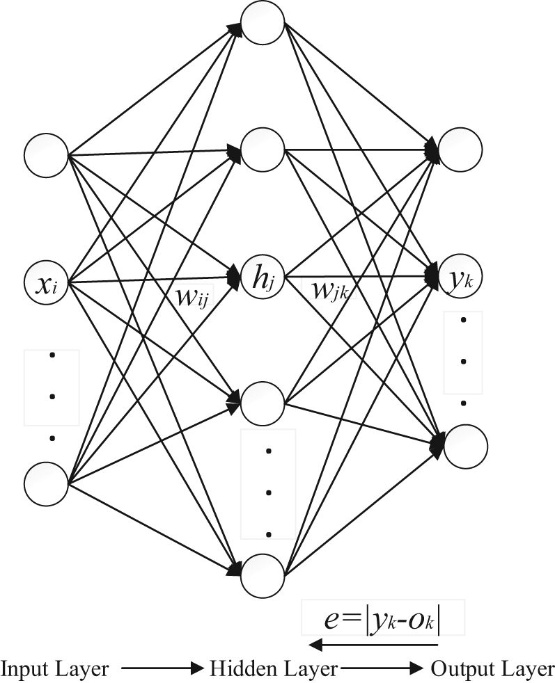
Basic BP neural network.
Standard BP algorithm weight adjustment rule is as formula (1)
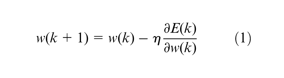
where k represents the run times, w is the weight of the model,
Self-adapting algorithm
The standard BP algorithm learning rate is a constant. In order to minimize the total error,
Self-adapting algorithm 11 is mentioned to improve the efficiency of learning process by automatically adjusting the learning rate of weight adjustment formula. When the new error is a certain ratio higher than the old error, the learning rate will decrease; when the new error is lower than the old error, the learning rate will increase. This method guarantees training the network at the maximum acceptable learning rate anytime.
The adjustment function of learning rate
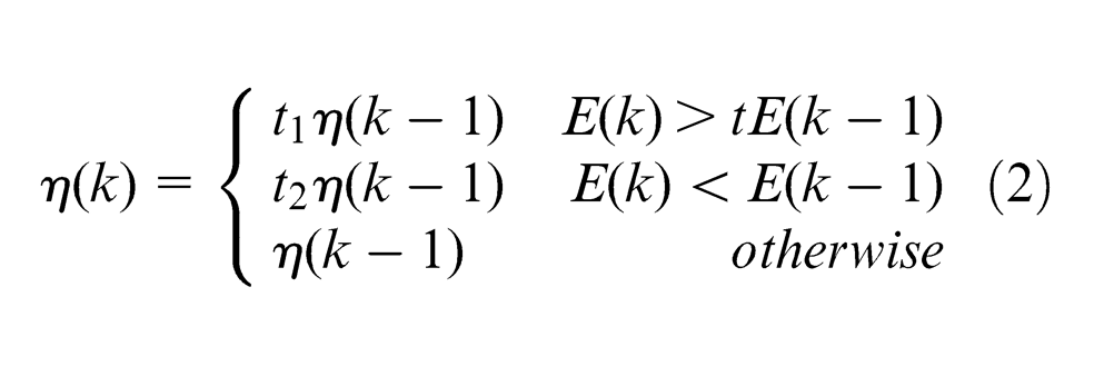
where
Additional momentum method
The additional momentum method transfers the influence of the previous adjustment of weight to the current weight adjustment formula through a momentum factor, which can not only reduce the BP training time but also ensure the stability of the process. 17 The momentum can adjust the weights toward the average bottom of error curved surface.
When the network weights enter the flat area at the bottom of error curved surface, the local gradient will become very small. The adjustment of weight is approximately the same at the iteration k and (k − 1), so as to reduce the network sensitivity to local details of error curved surface. In this way, the momentum can help to keep the network out of the error surface at a local minimum value.
Improved BP neural network
The self-adapting algorithm with additional momentum greatly shortens the training time and guarantees the stability of the training process. Improved BP neural network weight adjustment rule can be modified as formula (3)
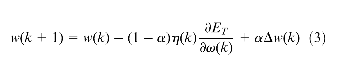
where
Theory of PSO algorithm
The PSO algorithm is originated from artificial life evolutionary computation theory. 20 In PSO algorithm, each particle is like a bird. The particle flies in the search space at a certain velocity and meanwhile dynamically adjusts its velocity and direction according to flying experience of its own and its companion. All particles have their fitness values that are determined by the objective function. Then, they can get their current positions and the best positions they have experienced (particle best, pbest) so far by calculating the fitness values. This experience is called the particle flying experience. In addition, each particle also knows the best position all the particles have experienced in the whole group so far (global best, gbest), which is called the companion flying experience. Each particle uses the following information to change its current position: 1, current location; 2, current velocity; 3, the distance between the current position and the particle best position; and 4, the distance between the current position and the global best position. Optimization search is carried out by such a group of randomly initialized particles in an iterative manner.
Algorithm description
Suppose a swarm in a d-dimensional target search space composed of m particles
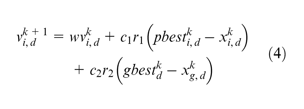
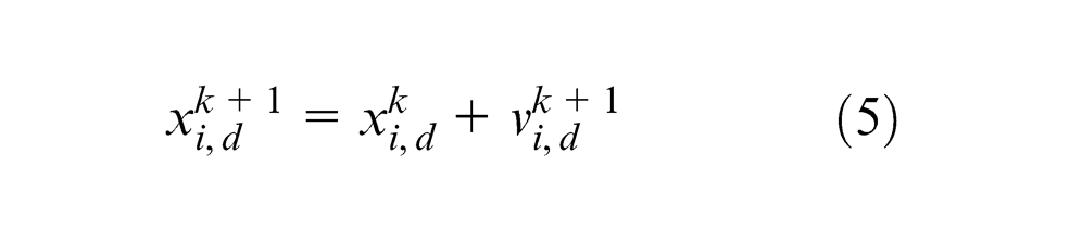
where k is the iteration number;
The
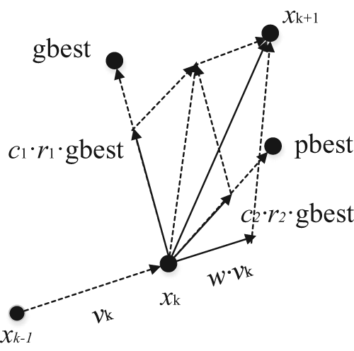
The particle position update.
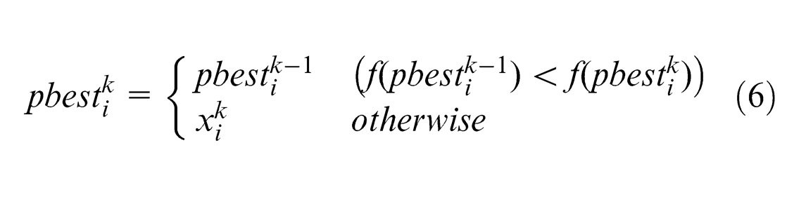
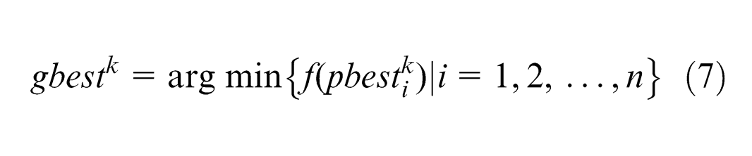
From Figure 2, it can be seen that the distance between particle x and gbest is becoming closer with the increase in the number of iterations. For the minimization problem, the smaller the objective function value, the better the fitness value. 22 Given function f, the update rules of minimization problem are as formulas (6) and (7)
Improved PSO algorithm
The inertia weight w is provided to control the global search ability and local optimization ability of PSO. A higher value of w helps particle to jump out of local optimum for the global optimization; a lower value of w is beneficial to the local optimization and can accelerate the convergence of the algorithm. An improved PSO by decreasing inertia weight with the increase in iteration is presented. The parameters of this algorithm are set as follows:
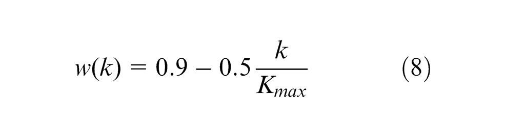
where
This algorithm has a higher inertia weight in the early iterations to guarantee the global search ability of PSO; w becomes lower later, so that the local optimization ability is strong to get a better convergence performance.
The basic steps of PSO algorithm
Step 1. Initialization: initialize the particle swarm position x in
Step 2. Calculate the fitness of each particle.
Step 3. Update the particle best of each particle according to formula (6).
Step 4. Update the global best of the swarm according to formula (7).
Step 5. Update the velocity and position of the particle according to formulas (4), (5) and (8).
Step 6. Judge whether the iterations meet the termination condition. If so, enter the Step 7, or else, back to Step 2.
Step 7. End, save the result.
PSO-BP neural network model for tool life prediction
In the actual machining process, tool life usually refers to the tool durability. It refers to the tool cutting time from the new or newly sharpened tool first into use to the tool is dull or broken. Boring, milling, drilling machine tools and computer numerical control (CNC) machining centers are the major machines used in flexible manufacturing system (FMS) workshop. Tool durability is proportional to the tool use coefficient, tool material and diameter and so on and inversely proportionate to the workpiece material coefficient, cutting velocity, depth of cut, cutting width, number of teeth and so on.
The traditional calculation of tool life 23 is given as formula (9)
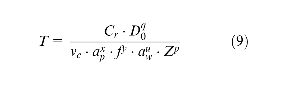
where
The relationship between tool life and influence parameters is highly nonlinear. This relationship can be more complicated with the influence of the machining environment. Formula (9) can hardly describe this relationship correctly. 24 BP neural network is simple, rapid and economical. Besides, it has the capability to approximate any nonlinear function with arbitrary precision. These characteristics are very suitable for tool life prediction. But BP neural network has its own weaknesses. It would easily fall into a local optimum and is slow in convergence and weak in generalization ability. By contrast, PSO algorithm also has the advantages of easy implementation, fast convergence and strong robustness compared to GA and ant colony algorithm. Considering the powerful global search ability and generality of PSO algorithm and the strong local search ability of BP algorithm, this article built the PSO-BP model by combining the PSO and the BP neural network to predict tool life. PSO is used to optimize the weights of BP neural network. It takes the influence parameters as input and the tool life as output of neural network. The weights are optimized by the improved PSO to narrow the search range, and then optimized by neural network for better convergence.
Steps of the PSO-BP algorithm
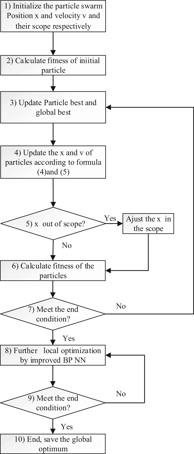
Figure 3 shows a flowchart of the PSO-BP algorithm.
Step 1: initialize the particle swarm.
The particles contain the information of the connecting weights and thresholds of the BP algorithm. Therefore, the topology of the neural network should be built according to the sample data and the function of the algorithm first. The number of the input nodes and output nodes are set by the “variable” and “dependent variable” number of the sample data; the hidden layers and its nodes are set through testing experiment or the former researchers’ experience. All the connecting weights and thresholds are encoded into a vector which is called the particle.
The particles have its fly rule and limited fly area. The parameters for the fly rule and fly would be set. These parameters include population size M, inertia weight w, learning factors c 1 and c 2, range of particle’s position and velocity, termination condition of PSO and BP algorithm. The initial particle swarm can be generated randomly based on the principle of uniform distribution. This principle guarantees the global search in the area.
Step 2: evaluate the fitness values of the initial particles.
The fitness function f should be established first. The function of f is to find the distance between the target and the current position. The distance is determined by the function f. A better function f can reduce the learning time and improve the precision of the result. The connecting weights and thresholds, which form the current BP model, are isolated from the gbest. For this PSO-BP model, the fitness function is used to compare the errors between the output values of the current BP model and the desired values.
Step 3: update the pbest and gbest.
For the initial particles, the pbests are set as the fitness of the initial particles; for the particles after k iterations, the pbests are updated according to formula (6). The gbests are selected from the pbests through formula (7).
Step 4, Step 5 and Step 6: update the particle velocity and position.
The update rules have been presented in formulas (4), (5) and (8). Both the adjustment of the velocity and the position are affected by the pbest and the gbest. Formula (8) is to keep the particles flying in the given area. The pbests and the gbests are updated again by calculating the fitness values of the new positions of the particles. This is a step-by-step process to find the optimal solution.
Step 7: judge whether the iterations meet the termination condition.
The termination conditions are usually set to the maximum iterations or a desired fitness value. If so, enter Step 8, otherwise, back to Step 3 to update the pbest and gbest again.
Step 8 and Step 9: train the BP neural network.
The global search of the PSO algorithm is over. The connecting weights and thresholds of the BP neural network are obtained. The improved BP neural network presented in section “Improved BP neural network” is trained to search the local minimum in the vicinity of the gbest. If the search result is better than gbest, update the gbest. The set method of termination condition is the same as Step 7.
Step 10: optimization over. Save the connecting weights and thresholds.
After these steps, a PSO-BP algorithm for the specific problem is presented.
Flowchart of the PSO-BP algorithm.
Model building
1. Build the topology of neural network
The choice of the network topology decides the performance of the neural network. 25 This work includes the design of input layer, output layer and hidden layers.
Input and output layer design
The tool life is influenced by processing mode, tool materials, workpiece materials, machining precision, tool diameter, tool teeth, depth of cut, feed rate, milling width, cutting velocity and so on. But in the actual processing, when sample data are enough, good learning samples can be obtained through the advanced screening conditions. 24 So, the non-numeric factors, such as milling mode, tool materials and workpiece materials can be selected as query conditions. The samples are queried in this condition. Therefore, six numeric parameters, including tool diameter, tool teeth, depth of cut, feed rate, milling width and cutting speed, are selected as the input nodes of network and tool life is selected as output node.
Hidden layer design
It had been proved that a three-layer BP neural network can simulate any n-to-m mapping. 26 So, this model selects the structure with a single hidden layer. According to Kolmogorov principle, 27 the number of hidden layer nodes is set by formula (10)

where I and N represent the BP neural network nodes of input layer and hidden layer, respectively. Set I = 6 and N = 13.
Therefore, the topology architecture of the neural network is 6-13-1.
2. Preprocessing of the sample data
Difference in the size of the training sample data has great influence on the convergence speed of the network, so the input and output sample data should be preprocessed (normalization processing) before training or testing. Formula (11) is used to compress the input and output sample data to (0.1, 0.9)
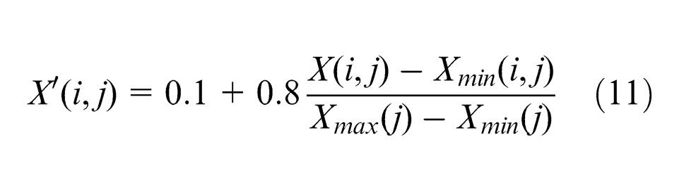
The results should be processed through anti-normalization to get the real prediction values of tool life.
Figure 4 shows the BP neural network model for tool life.
3. Parameter setting of the PSO algorithm
Set
4. Fitness function
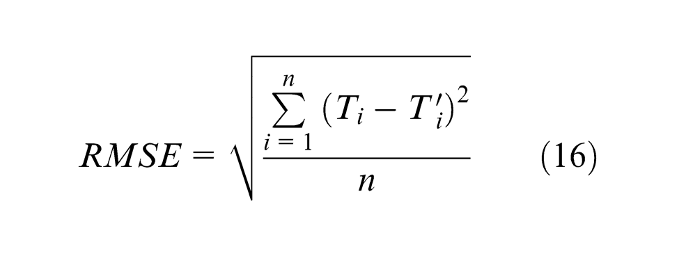
The root-mean-square error (RMSE) is a frequently used measure of the differences between the predicted values and the observed values. The RMSE represents the sample standard deviation of the differences between predicted values and observed values. The function of RMSE is given as formula (12)
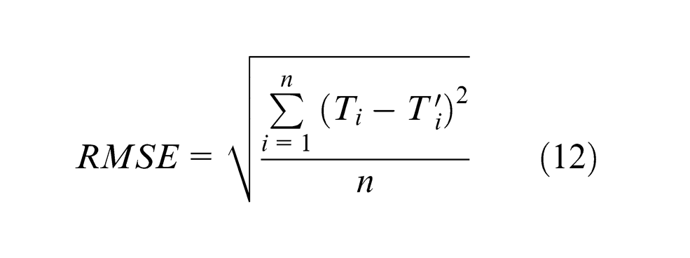
where
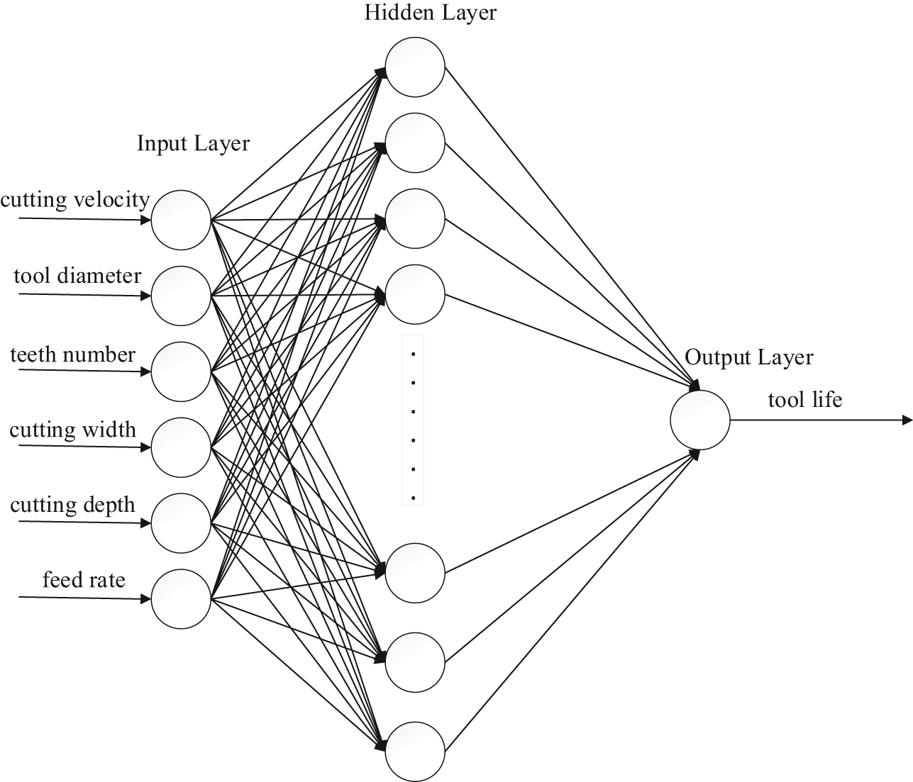
BP neural network model for tool life prediction.
The errors are squared before averaged, so the RMSE gives a relatively high weight to large errors. Therefore, RMSE is sensitive to the errors. This character guarantees both the accuracy and precision of the predicted value. The smaller the RMSE, the higher the accuracy and precision of predicted values. PSO is a way to find out the minimum. Hence, RMSE is chosen as a fitness function to guarantee both the accuracy and precision of the predicted value

Experiment and analysis
In order to verify the performance of this model, three simulation experiments for tool life prediction were carried out. One was conducted by PSO-BP model as this article presented, another was conducted by basic BP neural network and the other one was conducted by improved BP neural network mentioned in section “Theory of BP neural network.”
Sample data collection
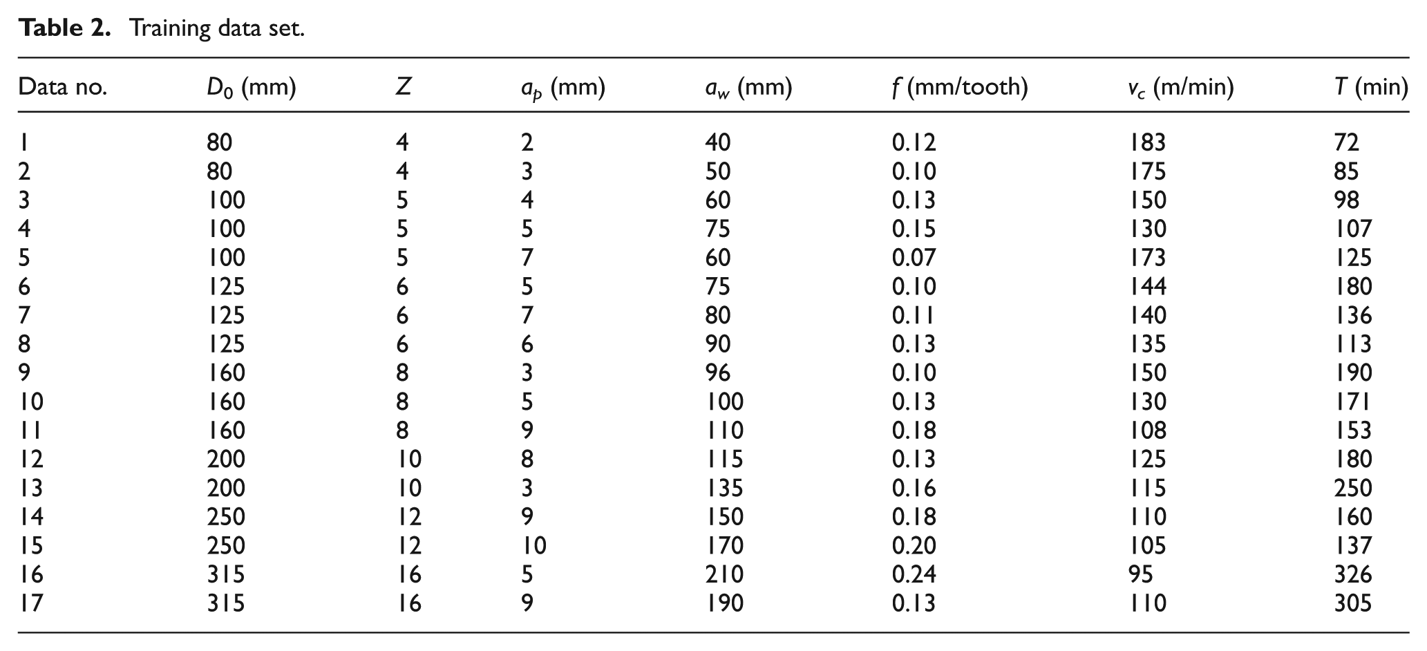
The most common cutters and workpieces were selected for this experiment. The most frequently used tools in FMS workshop are milling tools, among which face milling cutter and end milling cutters are the most commonly employed. Therefore, facing milling cutters were selected. The material of the cutters is YT15 cemented carbide; the material of workpieces is 45 steel; processing method is rough milling. The cutting conditions are shown in Table 1.
Tool cutting conditions.
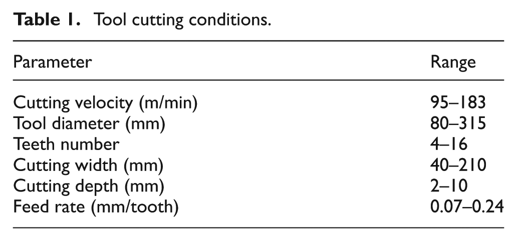
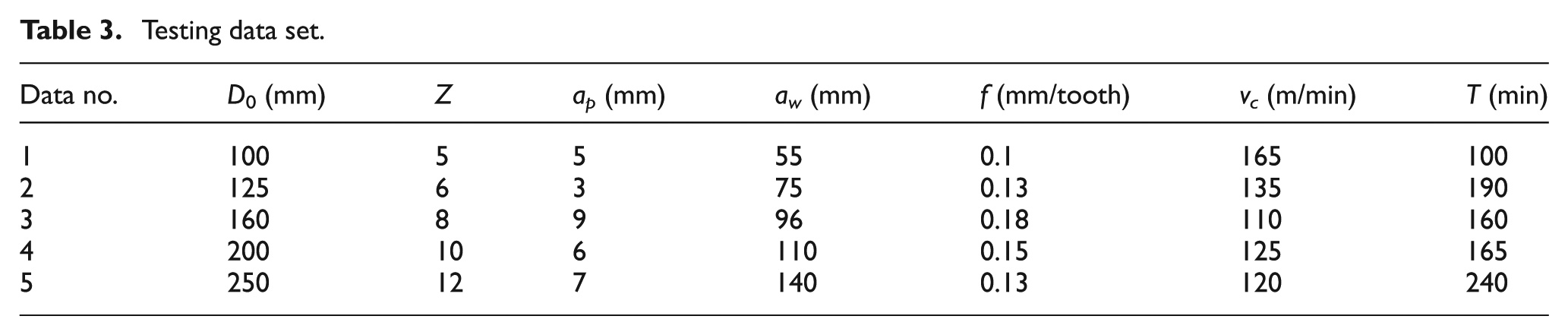
In all, 22 groups of sample data were included under this condition. Table 2 shows 17 groups of the sample data which are used for training the network. Five groups of the sample in Table 2 are used for testing the performance of the network (Table 3).
Training data set.
Testing data set.
Error measures
To assess the performance of the PSO-BP model, the following error measures were used:
Absolute error
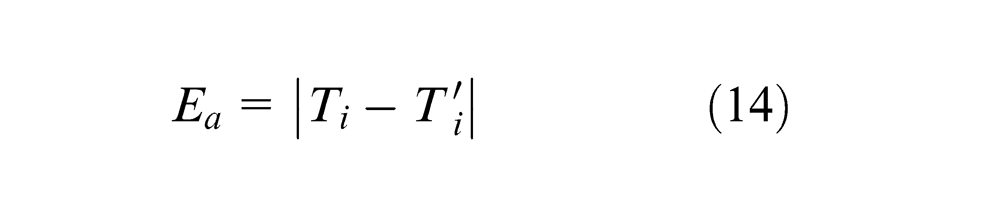
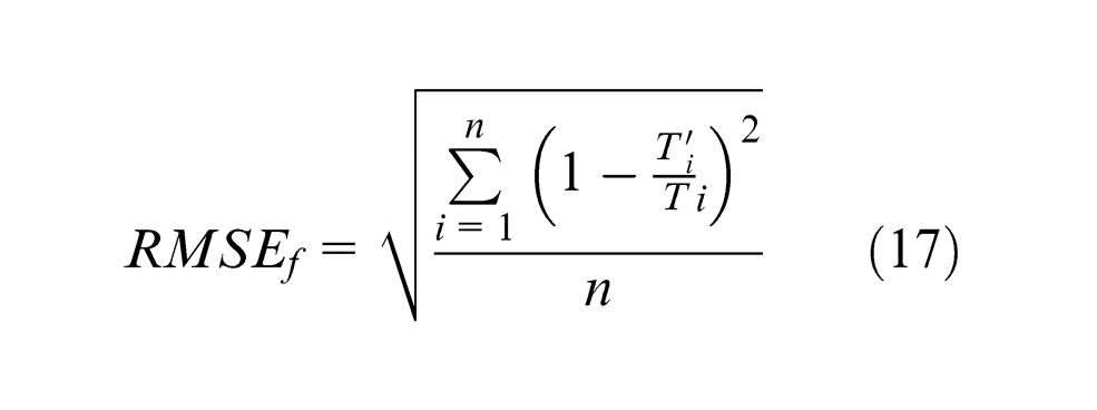
Fractional error
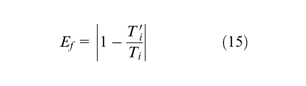
RMSE
Mean square fractional error
Simulation experiment and results
Environment of the simulation experiment
The simulation experiment about PSO-BP model, improved BP model and BP model was conducted 10 times in the computer. The computer environment used in the experiment was as follows: Intel
Parameter and process setting for the three models
The MATLAB programs of these three models were built by the parameters presented in Table 4 and section “PSO-BP neural network model for tool life prediction.” The values of the connecting weights and thresholds were trained by the training data set. The results were obtained by the trained models.
Results of the simulation
Table 5 shows the average predicted tool life of testing samples. Table 6 shows the detailed performance of the models. These performances were obtained by the statistic of all the outputs of the three models after 10 training. The average values of the errors, including RMSE, RMSEf , Ea , Ef and correct rate, are selected for the performance. The correct rate in Table 6 refers to the proportion of the predicted values whose absolute value of fractional error is less than 10% in all values. Figures 5–7 show the distribution of the predicted tool life.
The parameters of BP, improved BP and PSO-BP models.
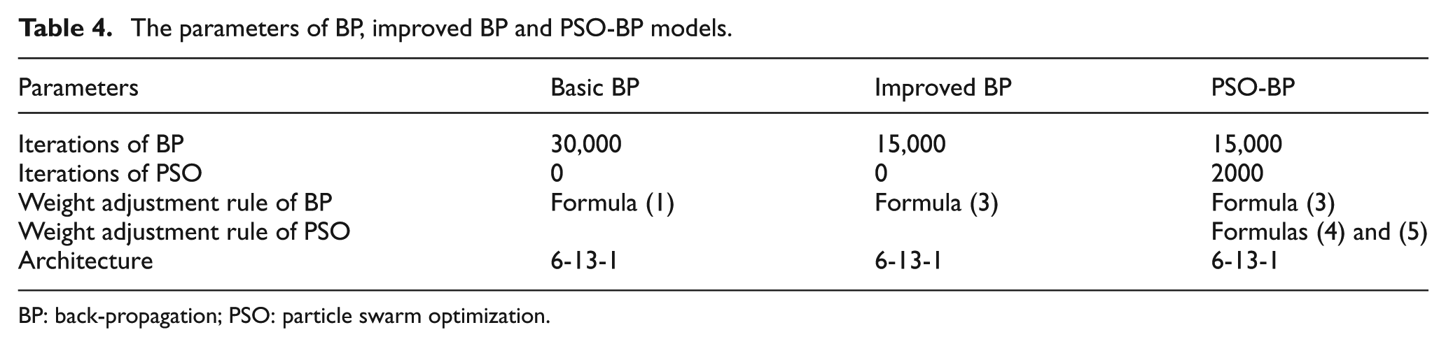
BP: back-propagation; PSO: particle swarm optimization.
The outputs of BP, improved BP and PSO-BP model.
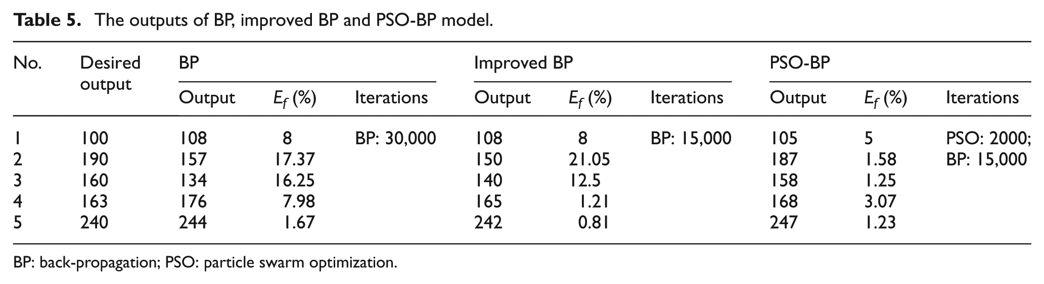
BP: back-propagation; PSO: particle swarm optimization.
Performance of BP, improved BP and PSO-BP models.
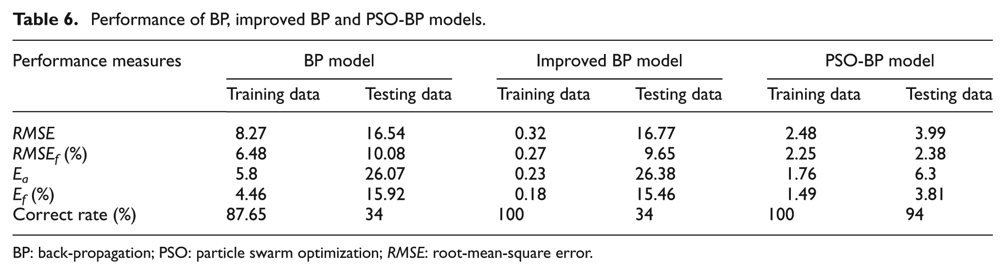
BP: back-propagation; PSO: particle swarm optimization; RMSE: root-mean-square error.
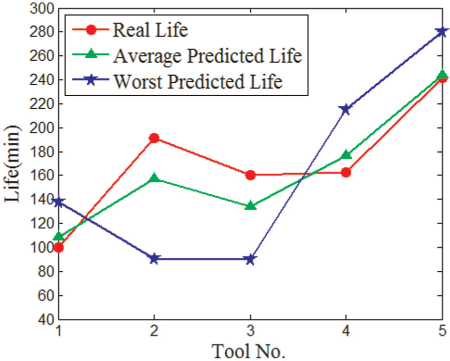
Life distribution of basic BP.
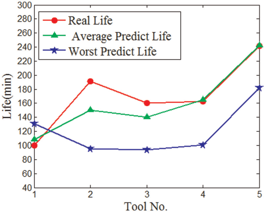
Life distribution of improved BP.
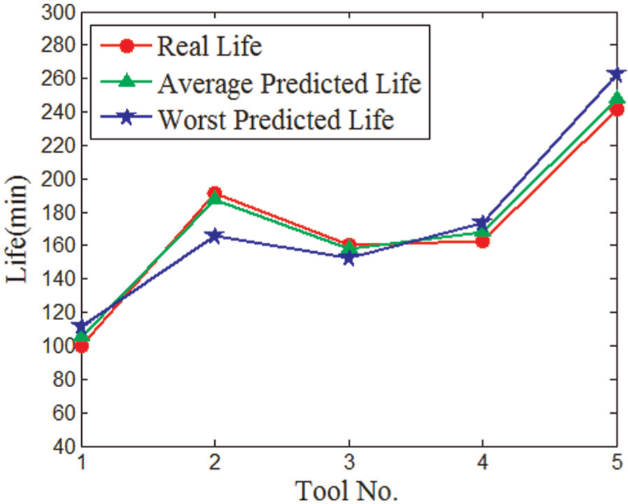
Life distribution of PSO-BP.
Analysis of experimental results
It can be seen from Table 5 that the life predicted by the PSO-BP model is better than basic BP model and improved BP model. The differences between the results of BP model and improved BP model are not significant. The number of iterations of PSO-BP model is smaller than that of BP model. The values of fractional errors of basic BP model range from 1.67 to 17.37. While the fractional error of all the testing data is less than 5.00% which is much smaller than the values of BP model. The less iterations and high accuracy show the fast convergence of the PSO-BP model.
The training data errors of basic BP model in Table 6 are relatively small which indicate the strong ability of nonlinear fitting. But the testing data errors are larger than the training data errors. These weaknesses reveal the low generalization ability of BP model. The training data errors of BP model are the smallest in the three models, but the testing data errors are not satisfied. The testing data errors are as poor as the error of the basic BP model. This proves the fast convergence but the low generalization ability of the improved BP model. All the errors of PSO-BP model in Table 6 are much smaller than those of BP model. The testing data correct rate reaches 94%. RMSE is an effective way to evaluate the accuracy and precision of the result. The 3.99 of RMSE shows the high generalization ability of PSO-BP model.
The average predicted life and worst predicted life shown in Figures 5–7 further proved the higher convergence and greater generalization capability of PSO-BP model.
Through data analysis and comparison, the convergence, robustness and generalization of neural network are greatly improved by using the PSO-BP model. The performance of the PSO-BP model is much better than that of the BP neural network. PSO-BP model is very suitable for tool life prediction.
The satisfied results of the PSO-BP model demonstrated that this model is applicable for tools with different diameters and cutting teeth.
Summary and conclusion
A reliable BP neural network model based on PSO algorithm is established in this article to predict the cutting tool life. This model takes the advantages of the global search capability of PSO and the complex nonlinear mapping ability of BP neural network. In this model, PSO algorithm is used to optimize the weights and thresholds of BP neural network before the training BP neural network. BP learning algorithm is further used to find the optimal.
The highly nonlinear relationship between affecting factors and tool life can be obtained through the utility of the complex nonlinear mapping ability of BP neural network. An effective method for tool life prediction is achieved by training the existing experimental and production data. The calculating process is a black-box operation which reveals the strong adaptive ability of PSO-BP neural network.
Theoretical analysis and simulation show that PSO-BP algorithm can effectively reduce the risk of falling into a local minimum value of neural network, in which the convergence, robustness and generality of the BP neural network are greatly enhanced.
A neural network expert system is established when this model is adapted in FMS tool management system and the sample data are saved to the database. Then, more tool information which can provide a dynamic tool sample database for PSO-BP tool life prediction model will be obtained. Furthermore, a dynamic update of PSO-BP model is achieved with the support of this database to improve the preciousness of life prediction.
In this article, tools with different diameters and teeth numbers are selected as sample data and predicted successfully by this model. This indicates that more affecting factors, such as the hardness of the materials and tools, can be selected with the support of the neural network expert system.
This model also provides an effective way for the optimization of tool machining parameters. In the machining process, in order to realize the unity of tool change time and improve production efficiency, the desired tool life can be obtained by adjusting the parameters affecting tool life. For selected tool and material, users can adjust the input parameters of cutting speed, depth and feed rate until the output results reach the expected tool life. The workshop production efficiency will also be greatly improved by combining this model with FMS.
Footnotes
Acknowledgements
Thanks to Zheqi Zhu for improving the language (English) of this article.
Declaration of Conflicting Interests
The author(s) declared no potential conflicts of interest with respect to the research, authorship, and/or publication of this article.
Funding
The author(s) disclosed receipt of the following financial support for the research, authorship, and/or publication of this article: The National Science and Technology Major Project (Grant No. 2012ZX04011-031), National Outstanding Youth Science Foundation (Grant No. 50925518), National Science and Technology Support Plan Subsidization Project (Grant No. 2012BAF12B09) and the Youth Science Foundation of National Natural Science Foundation (Grant No. 51005260) supported this research project.