Situation awareness via Internet of things and in-network data processing

Abstract

Computing on the edge of the Internet of things comprises among other tasks in-sensor signal processing and performing distributed data fusion and aggregation at network nodes. This poses a challenge to distributed sensor networks of low computing power devices that have to do complex fusion, aggregation and signal processing in situ. One of the difficulties lies in ensuring validity of data collected from heterogeneous sources. Ensuring data validity, for example, the temporal and spatial correctness of data, is crucial for correct in-network data fusion and aggregation. The article considers wireless sensor technology in military domain with the aim of improving situation awareness for military operations. Requirements for contemporary intelligence, surveillance and reconnaissance applications are explored and an experimental wireless sensor network, designed to enhance situation awareness to both in-the-field units and remote intelligence operatives, is described. The sensor nodes have the capability to perform in-sensor signal processing and distributed in-network data aggregation and fusion complying with edge computing paradigm. In-network data processing is supported by service-oriented middleware which facilitates run-time sensor discovery and tasking and ad hoc (re)configuration of the network links. The article describes two experiments demonstrating the ability of the wireless sensor network to meet intelligence, surveillance and reconnaissance requirements. The efficiency of distributed data fusion is evaluated and the importance and effect of establishing data validity is shown.

Introduction

Tens of billions of devices connected by Internet of things (IoT), which analysts predict will be deployed by 2020, will operate in our environment, enhancing our capability for acquiring real-time data for decision making and automating mundane tasks. The lowest layer of IoT will operate on low-power, low-bandwidth embedded networks, which conventionally have been called wireless sensor networks (WSNs). Due to the rapid development and spread of embedded computer technology over the last decade, sensor nodes are widely used and produce potentially abundant information for IoT applications. However, the disconnected, intermittent and limited (DIL) communication environment that these nodes often operate in make the usage of Internet-level communication solutions not applicable on the WSN level.

In order to manage the large data flows and to minimise the bandwidth requirements, novel paradigms such as data to decision (D2D) and mist computing (an extension of fog computing) need to be exploited. ¹ Traditional data aggregation ² is a predecessor of these paradigms, but in its classical form is not enough for IoT applications, because the traditional flow of data from network edge (sensor nodes) to centre (databases) remains. According to the D2D concept, ³ relevant data are identified in the network and delivered to decision makers and fashioned to their current data needs, which are derived from the specific decisions that they need to make. Mist computing characterises the architecture where computation occurs not only in the cloud but also in end nodes, such as sensor nodes. ⁴ Combining the D2D approach with the Mist Computing paradigm allows to utilise a large number of sensing nodes while overcoming technical bandwidth challenges and providing the consumers the required situation information with reasonable use of network resources. This article presents a military purpose WSN that follows these paradigms, brings computation to the edge of the network and makes results available to users directly, without being dependent on the cloud.

Successful deployments of WSNs have been demonstrated in a range of domains, for environmental monitoring applications in rural ⁵ and urban ⁶ areas, for infrastructure (bridges, buildings) structural health monitoring,^7,8 for early detection of natural disasters (such as forest fires, ⁹ landslides ¹⁰ and volcano eruptions ¹¹ ), for industrial monitoring ¹² and for various specific tasks such as object tracking, ¹³ perimeter or object security monitoring ¹⁴ and patient health monitoring. ¹⁵ In most WSNs, the data acquired by sensors are communicated and collected to a central server, where the data are processed and made available to potential users. Although actual communication paths for data are established at run-time, the overall structure of the network, types of data and structure of the central database are known at design time. Typically, in such scenarios, data processing, fusion and analysis are done at the server database level, not in the WSN itself. Inside the network data are usually processed only for aggregation, mostly for the purposes of optimising sensor power usage and network throughput.

A growing number of contemporary IoT applications require more from WSNs than simple data acquisition, (conditional) communication and collection to databases. For example, military applications, such as intelligence, surveillance and reconnaissance (ISR) systems, aim to improve the situation awareness of decision makers and expect pre-processed data that are already converted to human understandable form. Data collection to central databases, as used in typical WSNs for monitoring, creates overhead, potential bottlenecks and offers limited resilience. An additional aspect is that some of the potential WSN users, such as in-the-field military units, need situational information in a timely manner and would prefer to receive information tailored to their current information needs directly from the network to minimise delays and dependence on central infrastructure.

We outline the general concept and design choices of our solution for a military WSN that provides situation awareness to users on different hierarchical levels (from tactical to strategic operation). The architecture and operating concept follows a service-oriented approach and publish–subscribe principles. As such, users (e.g. in-the-field military units, autonomous network nodes such as unmanned aerial vehicle (UAV) and command centre analysts) task the sensor network directly and subscribe to data of their interest. There is no requirement to collect all raw data to a central database and access the data through this database, although a database can still be created and used (e.g. for post-operation analysis). This greatly contrasts the common approach to environment monitoring WSNs, where users access data as clients of a central database. The service-oriented architecture and publish–subscribe principles fit well for WSNs designed to operate in tactical military settings, considering the highly unreliable communication links and persistent shortage of bandwidth that these networks encounter. Allowing users to directly interact with sensors constrains the network less than general network-wide data collection and distribution via a central database.

Figure 1 presents a general overview of the different functionality of the designed WSN. Signal acquisition and initial signal processing are conducted on sensor nodes. The produced data are then transmitted to interim fusion or aggregation nodes which combine the distributed data into new data types and/or structures. It is possible to have several fusion levels before the results are presented to the end user. Three different in-sensor signal processing cases are demonstrated. First, sensor nodes capable of audio signal acquisition compute the angle of arrival (AoA) of measured sound waves based on the time difference of arrival (TDOA) method. Second, some of these sensors are also capable of performing in situ fuzzy classification of the measured sound source (we are classifying vehicles based on the sounds they emit). And third, a camera-equipped sensor node performs video analysis with the goal of locating and counting mobile foreground objects (personnel) captured on the video.

Figure 1.

Overview of the functionality of network nodes. Arrows indicate possible communication flows. A service-oriented middleware (ProWare) handles communication between nodes.

In-network data fusion and aggregation are demonstrated by special network nodes (fusion or aggregation nodes). Fusion nodes collect AoA estimates from sensor nodes and calculate the location of the sound source from the intersection of beams formed from the AoA estimates. We consider this to be in-network data fusion, since a new data type (location coordinate estimate) was created from another, different type of input data (AoA estimates). Location coordinate estimates can then be combined with fuzzy classification results to form new meaningful data structures (e.g. a data bundle comprising the classification result and location of a detected object). We consider this to be data aggregation, since data of different types are meaningfully grouped together and presented in a human understandable form. Additionally, data validity checking, necessary for the fusion and aggregation processes, is discussed.

Evaluating the efficiency of a military WSN is a challenging task, since performance depends highly on the configuration and size of the network, operational circumstances and usage (changing number of users and their requirements). However, we present experimental data of bandwidth usage in an urban setting and evaluate the efficiency of our signal processing and fusion algorithms in another experiment in military settings.

The WSN experiment presented in this article is still at a TRL 3–5 level. Therefore, some important topics, for example, energy-related issues such as energy conservation, usage optimisation and harvesting; scalability issues such as message routing, multi-hop communication and network congestion; security issues required by ISR systems such as message encryption and node hijacking resistance; and sensor synchronisation are not discussed in this article. However, we refer the reader to Egner et al. ¹⁶ and Turkmen et al. ¹⁷ for an overview of the possible security solutions.

Section ‘ISR requirements and situation awareness for military WSN’ describes ISR and military WSN requirements. Section ‘Related work’ gives a short overview of related work. Section ‘In-sensor signal processing’ presents three different instances of in-sensor signal processing. Section ‘Distributed data fusion and aggregation’ discusses in-network distributed data fusion, aggregation and data validity checking. Section ‘Communication architecture and principles of ProWare’ describes the proposed communication solution that meets (selected) military ISR and D2D requirements. Section ‘Demonstrations and experiments’ describes two field tests, one analysing the overall operation of the proposed WSN and the other focuses on bandwidth usage and quality of service. Section ‘Conclusion’ concludes the work.

ISR requirements and situation awareness for military WSN

The specific operational and functional requirements of military WSNs and overlying ISR systems call for a different architectural design and adaptive topology of WSNs compared to civilian examples. This section reviews some of these requirements. At the core of most of these requirements lies the need to have a situational understanding of events taking place in a monitored area. The situations (or rather the events) can be very versatile and numerous and it is not always clear at design and deployment time, what events can occur and need to be detected. Therefore, the section starts with a short explanation of how situations are handled and described.

We refer to our previous work on situations and give the definition of a situation as: ¹⁸

a situation is the aggregate of biological, psychological, socio-cultural, and environmental factors acting on an individual or a group of agents to condition their behavioral patterns. Here agent denotes natural (e.g. humans) or artificial (e.g. computing systems, or software-intensive multi-agents) agents, and environment means mix of natural or artificial environments.

Situations are treated hierarchically and defined by 3-tuples $S=\{S_p,S_t,S_a\}$ , where $S_p$ denotes a set of situation parameters and $S_t$ and $S_a$ comprise, respectively, temporal and spatial information about the situation. The parameters can be numeric variables or other situations, representing the hierarchical nature of situations. For example, the temperature of an area is a basic situation $S_{\mathrm{temp}}=\{S_p,S_t,S_a\}$ , where $S_p$ is a unit set holding the actual temperature value. A similar construct can be made for humidity $S_{\mathrm{hum}}$ . A higher level situation is composed of other situations either by fusion, for example, $S_{\mathrm{operation}}=\{S_p,S_t,S_a\}$ , where $S_p=f(S_{\mathrm{temp}},S_{\mathrm{hum}})$ is a function of temperature and humidity situations, or by aggregation $S_{\mathrm{weather}}=\{S_p,S_t,S_a\}$ , where $S_p$ is a two element set $S_p=\{S_{\mathrm{temp}},S_{\mathrm{hum}}\}$ . Here, $S_{\mathrm{operation}}$ is for instance the suitable environmental conditions for the operation of some device and $S_{\mathrm{weather}}$ is a set of weather parameters. Temporal and spatial information, $S_t$ and $S_a$ , are defined based on application needs and may include different information, for example, constraints, requirements and/or other data necessary for the interpretation of situation parameters $S_p$ . Further examples of defining situations are given in section ‘Demonstrations and experiments’.

The hierarchical principle for defining situations allow for a very dynamic and open system of situations to be created. This suits well with the changing nature of military situations and supports the design of military WSNs. The notation allows for general discussions over WSN requirements and feasibility at the preliminary design phase and technical discussions at the detailed design phase, while also transferring seamlessly between the different phases, when changes need to be made. High-level WSN architecture can be decided without the need to specifically define $S_p$ , $S_t$ and $S_a$ , these are only determined at the detailed design phase, where all relevant factors (environmental, technological, etc.) are taken into account.

The requirements for ISR situational information are as diverse as are the units and the levels of hierarchy in the military organisation. This article concentrates on in-the-field units who need situation awareness information relevant to them in a timely manner, preferably directly from network nodes as depicted in Figure 2 and in human understandable form. Information for situational awareness therefore needs to be provided already at WSN level utilising the capabilities of network nodes. Emphasis is put on requirements that are derived from highly dynamic ISR military situations and the corresponding complex data flows within WSNs. We exploit the design paradigms of mist computing and D2D paradigm which are about pushing computation to the edge of IoT network and bringing correct data in timely manner to the right decision makers.

Figure 2.

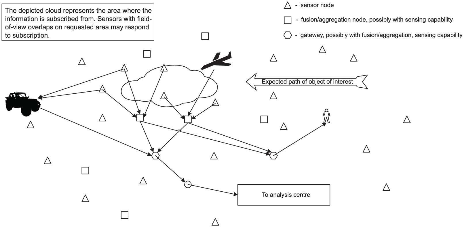
WSN deployment and dynamic formation of network links at run time according to the required situational information. Military units, such as ground patrols and unmanned aerial vehicles, acquire data directly from network nodes when in vicinity. When requested, data are also forwarded to analysis centre for online and/or offline analysis.

One of the main requirements, which differentiates military WSNs from typical civilian special purpose (scientific and commercial) WSNs, is the need for highly dynamic network structure – the ability to add or remove nodes and reconfigure communication paths on the go. In ISR applications, information collection is context based (i.e. constraints for information are contextual), therefore precise data requirements for tactical operations of military units are not known before WSN deployment and often change dynamically during operation. A WSN with fixed functionality and structure cannot answer to the changing needs. Sensors and communication paths for specific situational information need to be chosen and formed on ad hoc basis. Sensors may also leave these networks, as their power resources become depleted or they get destroyed, and new sensors, possibly with different functionality, may join the network according to the changing demands of the overlying ISR system. It is therefore not possible to design a complete sensor network for ISR applications, with fixed configuration, structure and predefined data flows. Rather, the system must accommodate dynamic run-time sensor discovery, tasking of data providers, that is, identifying and subscribing to available data sources (sensor and/or other information providers) and ad hoc formation of communication paths to cope with the changing goals and environment. As is described in section ‘Communication architecture and principles of ProWare’, sensors do not subscribe to data from specific data providers with their unique identification numbers, but rather subscribe to data according to its type, location, time and other parameters that describe (and give context to) the needed situational information.

Another requirement, from the point of in-the-field military units, is to be able to acquire data directly from nearby network nodes rather than connecting to a remote database. The reasons for this are that connecting to a remote database takes time, communication can be intermittent and the database may not have the latest data. Also all WSN nodes would have to constantly update the database, which consumes network bandwidth and takes time. As an alternative, distributed data aggregation and fusion must be performed at network node level to provide the necessary situational awareness to military units. Sensor and other nodes must be capable of carrying out the required signal processing, data fusion and aggregation calculations, while at the same time assuring that the data used are mutually conforming.

Performing in-network data fusion and aggregation in timely manner requires consistency of data collected from different sensor nodes in both temporal and spatial domains. In order to ensure the validity and usability of fusion and aggregation results, constraints must be applied to collected data. Spatial constraints, such as bounds to the area of interest, and temporal constraints, such as acceptable age of data, are defined within the subscription made to the WSN by the user. In either case, data providers, the different sensor nodes, must append all measured data with appropriate temporal and spatial metadata tags, which are later used in the data validation process. In addition, network communication layer must support in-time packet delivery (within the pre-specified delivery interval) or inform data provider and consumer of failure to (temporarily) meet these requirements during operation. The WSN presented in this article utilises a messaging syntax and communication protocol for WSN that facilitates satisfying the above described data validity needs.^19,20

The expected environmental conditions for tactical military WSNs are for the most part similar to those in typical civilian environment monitoring WSNs – sensor nodes are situated in harsh environments and need protection against the elements. Operational conditions, however, are different due to constantly changing military situation and the existence of malicious adversaries trying to disrupt network operation. Among other properties, it is desirable that sensor nodes be physically and electronically inconspicuous and if possible resistant to tampering, denial of service ²¹ and deception type of attacks. The latter properties that concern security and electronic warfare are outside the context of this article.

In conclusion, we identify five major requirements for tactical operation purpose WSNs:

1. Dynamic network structure and functionality is preferred along with ad hoc formation of communication paths.

2. Situation awareness should be created on WSN level.

3. Network nodes should be capable of in-sensor signal processing, distributed data aggregation and fusion.

4. It must be possible to assure that data are mutually conforming.

5. It should be possible to identify and task data providers at run-time using context-based data constraints.

The list is not conclusive but serves as a starting point for developing distributed in-network fusion systems. Sections ‘In-sensor signal processing’, ‘Distributed data fusion and aggregation’, ‘Communication architecture and principles of ProWare’ and ‘Demonstrations and experiments’ will present our solutions to these requirements and analyse the overall operation and feasibility of such a WSN.

Related work

We review related work in three parts, first focusing on general military WSN examples and requirements, then discussing signal processing on WSN nodes and finally reviewing distributed data fusion and aggregation in WSNs.

Common existing examples of military tactical WSNs operating on the edge of ISR networks are either highly specialised or based on commercial off the shelf systems (COTS) that are slightly ruggedised in terms of hardware and software, as compared to those used in civilian applications. (See, for example, the SPAN system from Lockheed Martin or the MicroObserver system from Textron Systems.)

Many civilian WSN, for example, those applied in manufacturing and industrial control, have reasonably good time-aware behaviour, that is, the ability to handle time-critical data and time-sensitive communication. Overviews of such systems can be found in Kopetz ²² and Zhao. ²³ Providing information in a timely manner is a necessary property for military WSNs and having temporal knowledge of information communicated in the network is the basis of creating correct situation awareness. However, the drawback of majority of civilian applications is that WSNs are assumed to have a fixed structure, fairly reliable end-to-end communications, capability of time synchronisation in nodes and that they operate on fixed rules and goals.

Military tactical WSNs, as a rule, must cope with disruptive communication and random communication delays, ²⁴ changing topology and composition of network, ³ dynamically changing rules and goals ²⁵ and asynchronously operating heterogeneous nodes. Tactical WSNs must be disruption-tolerant networks (DTNs) that can cope with the fragmentary connectivity of nodes, no guarantee of successful end-to-end message transfer and malicious cyber-physical attacks. ²⁶ The WSN experiment presented in this article does not specifically tackle the problem of unreliable communications, but network delays, disruptions and changes in topology are covered by the discussed service-oriented architecture and online data validity checking.

Due to listed discrepancies, COTS systems (and civilian WSNs) are most efficient in situations where the network operates in a stationary environment, for example, perimeter monitoring and control. ²¹ As one of the ways to tackle specific military requirements, several middleware solutions for WSNs have been developed (an example can be found in Pham et al. ²⁵ ) that implement service-oriented concepts known from Internet domain. Examples like publish–subscribe concept, service-oriented architectures and service provider discovery are gradually being implemented for WSNs. A survey of service-oriented middleware solutions for WSN can be found in Mohamed and Al-Jaroodi. ²⁷

In-the-field military units need timely situation awareness. Creation of situation awareness therefore starts on WSN level utilising the capabilities of the sensor network. Distributed data aggregation and fusion are the methods of choice in military context, since the alternative of remote data analysis requires central data collection, which consumes network bandwidth and time.

Signal processing in WSN sensor nodes

Features, such as in-sensor signal processing and in-network data aggregation and fusion, are not new to WSNs nor are they military WSN specific. Two audio signal processing cases are considered in this article – sound wave direction of arrival estimation and sound signal–based classification of signal source. Detecting the location of objects based on the different physical waves they emit into environment is typically based on the TDOA of these waves to detectors. Popular algorithms for this purpose are MUSIC and SRP-PHAT, both of which have been utilised also for WSNs.^28,29 The latter example also demonstrates that while a lot of existing systems use general-purpose computers for signal processing, examples with low computing power sensor devices also exist. Applications that benefit from those methods include target tracking and shooter localisation for instance. ³⁰

Classification of objects based on assessing characteristics of emitted sound signals is another well-studied signal processing area and its application in WSNs for low computing power devices is an emerging trend.^31–33 Until a short time ago, wireless sensor nodes were not powerful enough to perform feature extraction from measured signals and to run conventional classification algorithms. Although today’s technology facilitates advanced signal processing, the issue of training the classifier (regardless of whether it uses neural networks, fuzzy classifiers or some other methods) remains. Classifier training is still hard to perform at run-time on currently available sensor devices or other WSN nodes. In our experiments, the training was done beforehand and sensor devices were deployed with the required class feature vectors installed.

Distributed data fusion and aggregation in WSN

WSN data aggregation techniques have developed hand in hand with the advancement and spread of WSN technology. The primary motivation behind data aggregation has been energy efficient data acquiring in order to extend network lifetime and enhance quality of service of WSN. ³⁴ Different data collection and processing schemes arrange that not all data are individually transferred to the network sink, but instead related data are accumulated temporarily somewhere in the WSN, where it is aggregated and only the results are forwarded to the sink. This reduces the amount and length of messages passed and subsequently saves energy and bandwidth. Use cases of data aggregation in WSNs include Jo et al. ⁸ and Ramesh. ¹⁰ The data aggregation we present does not only serve the purpose of saving energy, it also aims at enhancing the situation awareness of data consumers by combining different types of sensor data characterising a particular event detected in the WSN. Majority of WSN in-network aggregation, however, focuses on aggregating only data of the same type.

Data fusion also serves the purpose of enhancing situation awareness of the data consumer. The difference between data fusion and data aggregation is that different data types of sensor readings are not combined into a bundle, but instead are fused into a new type of data.

Data fusion in WSNs can be carried out locally, where a sensor node comprising different types of sensors fuses the data acquired from sensor readings and communicates the fusion result to consumers. In the case of distributed data fusion, the data from respective sensor nodes are collected by a prefixed sensor/fusion node that performs the fusion process and distributes the result to data consumers. Examples of distributed data fusion in WSNs are described in Mayk et al., ³ Bahrepour et al. ³⁵ and Lai et al., ³⁶ where events detected and sensor readings collected by individual sensor nodes are assembled by a fusion node. These references do not discuss the consistency and validity of the inputs for the fusion algorithms. In case of large ad hoc sensor networks and especially networks for ISR solutions, it is important that the consistency and validity of the fused information is analysed online. ²⁰

In-sensor signal processing

Computing on the edge of IoT requires that the computation is moved from the cloud to the network and as much as possible to the sensors themselves. This section will give an overview of in-sensor signal processing and describe three different cases of in-sensor signal processing that we have currently utilised in our WSN experiments. This section gives an overview of the three different cases of in-sensor signal processing that were utilised in WSN experiments presented in this article. The three applications were identifying and counting objects in video-streams, classification of objects based on sound signals and estimating the direction of arrival of sound signals (to sensor node). The choice of applications was motivated by ISR requirements, for example, the need to detect, count, classify and position objects (events) found in the environment. An example of a use-case scenario for these applications is described in section ‘Demonstration of system operation in military setting’. For each application presented in this section, signal processing was done locally on appropriate sensor nodes using local data acquired by the node itself. No additional information or data from outside were needed once operation had started.

The difficulty of performing in-sensor signal processing lies mainly in efficiently coping with the limited resources and constrained computational power of WSN computing devices. The specifications and hardware of used sensor nodes is presented in section ‘Demonstration of system operation in military setting’.

Automatic object counting

Information extraction by image processing is a resource-intensive task and is usually infeasible in the resource-limited WSN nodes at the edge of IoT. The described sensor node is equipped with a camera and applies signal processing methods to count moving objects by separating mobile foreground objects (e.g. people) from relatively static background in the field of view (FOV) and counts the average number of those foreground objects in a prefixed time period. This method does not classify detected objects and thus requires less computing resources. It can be implemented even in low-power sensor nodes. The output of the sensor is the count of detected objects and the temporal interval between the object detections. This result is communicated to the subscriber of these data (e.g. a fusion node).

The working principle of the object counting algorithm is to follow objects that are considered to be foreground of an image. The movement history of these objects is stored as a vector within a ‘Track’ data structure, one element for every input frame while the object is visible. Each element includes a convex contour around a foreground object and feature points within that contour that can be used to follow the object.

The image processing software combines well-known algorithms implemented in OpenCV library. Steps of the algorithm are shown in Figure 3. Every input frame is fed to the adaptive Gaussian mixture model background subtraction algorithm. ³⁷ Algorithm proposed in Suzuki and Abe ³⁸ is used on the resulting binary image of estimated foreground areas to find contours of foreground objects. An example is depicted in Figure 4(a), where foreground objects are circled with red contours. Contours that are too small, large or unusually shaped are rejected. The initially found contours will be replaced by convex hulls (blue contours in Figure 4(a)) around those contours. ³⁹ This simplifies some of the following calculations. Meanwhile, a FAST corner detection algorithm ⁴⁰ finds good feature points to track. Feature points that fall within convex contours are combined with those contours to create new Tracks (see Figure (b)). If the contour of a new Track has overlap with existing Tracks, then it will be merged into the older Track with the greatest intersection (notice the different shape of a Track contour, pink in Figure 4(b), and a convex contour, blue in Figure 4(a)). Merging combines contours and feature points of both Tracks. Tracks will be updated by following their feature points using optical flow algorithm (implementation proposed by Bouguet ⁴¹ based on Lucas and Kanade ⁴² and Lucas ⁴³ ).

Figure 3.

Principal steps of the object counting algorithm.

Figure 4.

A video frame after different image processing steps: (a) frame after background subtraction and contour creation around foreground objects (black areas – foreground objects; red contours – initial contours; blue contours – convex hull of initial contours) and (b) black-and-white frame with two Track objects (pink and purple). A Track object consists of a convex contour and feature points for tracking associated with that contour.

Acoustic signal-based fuzzy classification

In-sensor classification of objects (different military vehicles in this case) is performed by analysing the sound signals emitted by the objects of interest. Classification is one of the basic tasks in pattern recognition and data analysis, and it is performed by analysing the training data set to develop an accurate class description or model for each object present in the training data set. These models are then used to establish class labels to new data for which the class labels are unknown. The training data set that is collected from previous experiments with known vehicle types consists of multiple instances each tagged with a class label and having multiple attributes. For classification purposes, we use a fuzzy rule-based classification algorithm, ⁴⁴ because of its ability to deal with imprecise data, flexibility of the decision boundaries, because it has low resource requirements and the generated rules can be interpreted by a human if needed.

The classification procedure runs on microphone sensor nodes in parallel with AoA calculations described in section ‘AoA of acoustic sound waves’. The classification sequence is depicted in Figure 5, it takes as input a single acoustic signal frame from one of the microphones of the sensor array. The process starts with signal acquisition – the continuous analogue signal from the microphone is sampled and quantized by an analogue-to-digital converter (ADC). The one-dimensional digital acoustic sound signal does not provide rich enough information context by itself so it undergoes a procedure of signal analysis both in time domain and frequency domain to provide relevant attributes calculated for each short signal frame of 2730 samples, sampled at 20 kHz. Time domain signal analysis focuses on the shape and amplitude of a signal (in our case the root mean square energy is computed) and is well applicable to weakly oscillating and harmonic signals. If the signal is non-harmonic or highly polluted by noise, which foremost influences the signal amplitude and shape, time domain features (such as zero crossing rate, auto-correlation and root mean square energy) are less useful.

Figure 5.

Classification procedure.

The acoustic noise patterns that can be collected with sensors in the vicinity of moving vehicles consist of multiple components, including noise produced by the engine, exhaust system and tires, ambient noise from wind and rain may also be present. The harmonic nature of the engine noise is therefore seldom detectable and parameters of the overall spectral shape and energy distribution describing the vehicle noise patterns are used. These may include choosing band energies of 10–15 sub-bands in the interval of 10–3000 Hz, spectral centroid, spectral roll-off, spectral slope parameters and so on. The feature extraction both in time and frequency domains is explained in our previous works.^45,46

The sound patterns of passing vehicles are not consistent and depend on the distance, trajectory and type of a vehicle. As the vehicles under test produce a significant amount of noise, it is acquired even from a distance where the patterns are distorted and can cause classification errors. In order to minimise these errors, a minimum signal root mean square energy threshold is selected, which must be exceeded for the classification process to start.

AoA of acoustic sound waves

In addition to being able to detect, count and classify objects of the environment, it is desirable from ISR perspective to be able to estimate the location of detected objects. Location estimation is also performed based on the noise (sound signals) that objects emit and is computationally divided into two parts: estimating the AoA of sound waves at individual sensor nodes and combining the individual AoA estimates of several nodes into a single (or multiple) location estimates. The latter part is discussed in section ‘Location estimation’.

The direction of arrival of sound waves to a sound sensor is found using at least two microphone elements, placed at different locations, and calculating the TDOA of sound waves to either microphone. By knowing the location of either microphone, the TDOA and the approximate speed of sound waves, it is possible to find the direction towards the source of the sound waves. TDOA is found by cross-correlation of the measured sound signals, it is the delay between the signals. Once the delay is known, the direction is calculated as

$$\phi =\arcsin \frac{\Delta k/f_s·c\left(T\right)}{l}$$

where $\Delta k$ represents the delay in samples, $f_s$ is sampling frequency, l is distance between microphones and $c\left(T\right)$ is the speed of sound waves in air, which is a function of air temperature T. The orientation of angle $\phi$ , with regard to microphones, can be seen in Figure 6(c). The quality of the result mostly depends on the sampling rate and distance between microphones.

Figure 6.

Sensor field-of-view sensitivity based on sampling speed and microphone distance (top) and angle of arrival of sound waves (bottom): (a) 4 kHz sectors, (b) 20 kHz sectors and (c) sound-wave arrival and angle orientation $\phi$ . ³⁰

The method is implemented on two different platforms. The first, Atmel ATmega128RFA1 microcontroller based platform, has two microphones and samples each microphone at 4 kHz. The second, BeagleBoneBlack (BBB)-based platform, has six microphones and samples each microphone at 20 kHz. The six microphones are placed linearly with equal distance from each other and the extra number of acquired signals helps increase the accuracy of cross-correlation. The FOV of the sensor is $180\circ$ for both platforms. It is divided into discrete, non-equal segments as depicted in Figure 6(a) and (b). Sampling speed and distance between microphone pairs determines the number of segments. A sampling speed of 20 kHz enables a much denser segmentation of the FOV and thus the accuracy of angle estimation is much better for BBB platform.

Distributed data fusion and aggregation

In-sensor signal processing constitutes one half of computing in the edge of IoT, the other half being data fusion and aggregation. In our interpretation, the latter two differ from signal processing by the fact that for fusion and aggregation data are gathered from multiple functionally disparate and spatially distributed sources and need to be checked for compatibility before processing. Compatibility is currently checked against temporal and spatial parameters of the collected data, that is, the data from different sensors must originate from the same physical area and time period if it is to describe the same environmental event (or object). Of course other parameters can be considered, depending on the needs and requirements of the system. For example, adding confidence estimations to complicated sensor measurements (such as classification) or accuracy values (for AoA estimations) so that the fusion and aggregation mechanisms can pick the most reliable data for processing.

An example of distributed data fusion, presented in this section, is calculating the location of objects detected in the environment by angle estimates received from different sensor nodes. Distributed data fusion distinguishes from data aggregation in our work by the fact that a new data entity (object location, a geographical coordinate) is defined using other data types (angles and sensor node coordinates) as input. Distributed data aggregation is considered to be combining different data from different sources, which describe the same environmental event,into a meaningful bundle, but no new data are created. This approach expands traditional data aggregation in WSN data collection applications, where for bandwidth optimisation purposes usually only the same type of data is aggregated (i.e. at certain nodes in the collection chain the mean, minimum, maximum or other values are found for the collected data and only those results are forwarded).

Location estimation

Individual microphone array sensors alone can estimate the direction to a sound source from their position, but cannot effectively determine the distance to, and therefore also the location of, the source. A location estimate can be established, however, by several sensors in the same area by combining their direction estimates. Special fusion nodes are dedicated to this task, although in principle any sensor or other type of node can take up this task, if it has the necessary resources.

The fusion process is depicted in Figure 7(a). First data are collected from all sensor nodes, which have detected a sound event. The data include the location of the sensor node (geographical coordinates), the measured direction estimate (a geographic bearing) and metadata such as sensor sensing range and a time-stamp indicating the age of the measurement. Based on the age of each measurement, compatible sound event instances are found and only these are analysed together. Next, beams are formed along all the direction estimates and intersection points of these beams are found. Due to the discrete nature of AoA calculation procedure (see section ‘AoA of acoustic sound waves’) and other inaccuracies of input data, all the beams will never intersect in a single point. Rather, a cluster of intersection points emerges and the density or sparsity of this cluster determines whether the result should be considered a valid location estimate or not. It is also checked that intersection points fall within the FOV of the involved sensors, intersection points out of range of the sensors are not considered. The forming of clusters of intersection points may also be guided by classification results if they are provided together with AoA estimates. This enables fusion algorithm to separate the intersection points according to provided classes.

Figure 7.

(a) Location estimation process and (b) example of location estimation in WSN for two sound events.

An example of a location estimation situation in a WSN is depicted in Figure 7(b). Two sound events are detected at the same time, one on the left side of the WSN by four sensor nodes and the other on the right side by three nodes. All seven sensors forward their direction estimates to the fusion node in the middle, which ideally should separate the estimates into two groups, left and right. There are many ways to do this and in our approach we consider the sensing range of sensors coupled with their direction estimates, to find nodes with converging results. Currently, the location estimation result is represented as a rectangular area encircling the cluster of intersection points, as depicted in Figure 7(b), from this cluster, a single geographical coordinate can be computed, which is a weighted average of the intersection points in the cluster.

However, the location estimations of moving sound sources and separating between several different sound sources may still be opportunistic and requires further analysis due to the nature of sound wave propagation and rapidly changing environment. The exact limitations have not been tested during the experiments described in this article.

Aggregation

Only one aggregation combination is used in the WSN experiment, that is, combining three different types of information from different sources into a bundle. The information that is aggregated is the number of detected objects, classification of these objects and their location estimates. The same way as for distributed data fusion, compatibility of information is verified based on data age and spatial distribution. The composed information bundle receives a time-stamp of its own, to represent the time of its creation.

The benefit of data aggregation is twofold: to optimise network resources, by having only one (slightly larger) message to deliver rather than several, and to provide better situational awareness to end users. Having data aggregation capability at the very edge of the network enables users to acquire information from network nodes directly while in-the-field without having to make database queries. This is an important operational advantage for military ISR applications.

Data validity for fusion and aggregation

In order to ensure the correctness of in-network data fusion at different network levels, the data validity must be re-evaluated at each level. Online validation service provided by the ProWare middleware realised as MURP modules (described in section ‘Communication architecture and principles of ProWare’) requires that the data produced are augmented with additional metadata for ensuring temporal and spatial correctness. According to ProWare concept, the data validity is checked on both sides, first the data producer decides if it is able to provide the data according to the consumer requirements and second the consumer evaluates the data validity when it arrives. ²⁰ A WSN simulation described in Preden et al. ⁴⁷ shows that ProWare data validation concept considerably helps to reduce the total number of packets exchanged in WSN. In the following some of the more important temporal and spatial validity aspects for current experimental WSN setup are described.

Checking the correctness of data in the temporal domain requires that a sensor reading is augmented with two pieces of time-related metadata: validity interval and the age of the sensor data. The age of data is represented in relative timescale and is incremented by each network node by the time it has spent on processing the data. The validity interval describes an interval when the data are usable and is decided based on the knowledge about the physical phenomena being measured. In case the validity interval expires before the message reaches the consumer, the message is dropped. Using the age of the measurements, computed by sensor platform and incremented by each node on communication path, it is possible for the data consumer (e.g. fusion node) to compute what was the original data acquisition time at the specific sensor and use it for example when evaluating the simultaneity of multiple arrived measurements.

A generic example of distributed sensor communication is presented in Figure 8. Black rectangles on the sensor timelines ( $t_{S_1}$ , $t_{S_2}$ , $t_{S_3}$ ) represent the duration of signal processing on each sensor node, and arrows indicate the transport times. The packets reach the fusion node at times $T_{S_1}$ , $T_{S_2}$ , $T_{S_3}$ (on timeline $t_{\mathrm{FN}}$ ). On the fusion node ProWare estimates the total transport and processing times of each packet incoming from $S_1$ to $S_3$ , denoted by rectangles $T_{\mathrm{proc}}$ and $T_{\mathrm{transport}}$ . The event detection times are then aligned to the estimated time moments ${\hat{T}}_{S_1}$ , ${\hat{T}}_{S_2}$ , ${\hat{T}}_{S_3}$ and compared against the simultaneity interval $I_{\mathrm{simultaneity}}$ (on timeline ${\hat{t}}_{\mathrm{FN}}$ ). Figure 8 illustrates that the processing time and packet transport time for each sensor node may be different, which results in the packets arriving out of order and too far apart to be included in the same simultaneity interval. Therefore, without proper temporal validation event, concurrency is not guaranteed to be established. Processing delays, originating from sensor platform non real-time operating systems, clock jitters and drifts, ad hoc WSN transmission scheduling, limited bandwidth and packet collisions within the network – all can unexpectedly disrupt WSN communication. The questions of how precisely the original time moments of measured events from different sensors are estimated, and what is the maximum simultaneity period, required for fusion, are the topics of future research.

Figure 8.

Temporal alignment and the simultaneity interval.

In spatial domain, the sensor data are augmented by validity metadata which are the sensor position and computed confidence value for the relative bearing to the noise source. This confidence is used by the fusion process in order to derive the confidence of the outcome of the fusion process. The subscription for the data broadcast by data consumer contains the area information from where the data is needed – this is spatial constraint. The data provider evaluates this spatial constraint against the sensor position and the area in the sensor FOV and in case the spatial constraint is satisfied (together with temporal constraint) the sensor-node will provide the data.

Communication architecture and principles of ProWare

The communication layer that ties together all the heterogeneous sensors provides data exchange and enables distributed fusion and aggregation in WSNs is a multi-functional middleware. There are numerous existing examples of middleware, with different capabilities and properties, a survey paper to some of them was referenced in section ‘Related work’. We discuss the principles, hardware and software of the middleware layer developed by our team. ⁴⁸

Extracting valid situation information from a WSN relies on correct acquisition and interpretation of sensor data as well as correctly combining and evaluating data collected from different sources. In dynamic, quickly changing environments typical to military operations, only relevant data must be exchanged in a timely fashion and guided by real needs. Central data collection (to a remote database) and distribution comprises a lot of redundancy and is often not flexible enough to provide the necessary timely situation awareness. An alternative approach is one, where service agreements between data users and providers are established at run time, based on actual needs. In this case, communication links are formed locally in ad hoc manner, increasing system robustness and efficiency. The above described procedures ensure the validity of communicated data (its correctness and relevance upon arrival to consumer) over unreliable links with unknown delays.

Considering the described requirements to WSNs used in ISR applications, we describe a solution ⁴⁸ that facilitates run-time data provider discovery and linkage to consumers, setting constraints to subscribed data, end-to-end transfer timing, tagging of exchanged data with metadata tags and checking data validity. The solution is in the form of a stand-alone communications module (custom design transceiver), which comprises software components, referred to as ProWare, ²⁰ and a hardware platform, referred to as MURP. (MURP has been designed, developed and produced by Thinnect Inc in cooperation with Research Laboratory for Proactive Technologies, Tallinn University of Technology.)

The general principle of how network nodes are connected through MURP transceivers and how communication is organised by ProWare is depicted in Figure 9. Nodes are equipped with the MURP module and all data transmitted and received passes through the module. MURP connects to nodes over a serial interface and enables creating a unified network from devices that may otherwise be different in nature (i.e. with incompatible software and/or hardware). ProWare provides the necessary communication services. These include handling data requests (in the form of subscriptions), establishing service agreements with suitable data providers and facilitating the delivery of produced data to consumers. It absolves the sensing and fusion applications running on network nodes from locating and contracting data providers themselves. Nodes need only to specify the type of data they produce and data they consume (when the need arises) and ProWare is responsible for arranging the communication. A node may be both a consumer and a provider, depending on the situation and on its functionality. In Figure 9, node 1 is a data consumer for node 2 and a data provider for node 3.

Figure 9.

Network nodes equipped with MURP transceivers forming communication links through ProWare.

ProWare also supports setting constraints (temporal and spatial) to data subscriptions, meaning that data consumers can impose restrictions (e.g. location – from where data are acquired, age – how fresh data must be) to specify what kind of data is acceptable to them. On the producer side data are tagged with necessary metadata tags (time and location of production) and upon arrival to consumers their validity and the satisfaction of subscription constraints are checked. Constraints are not limited to temporal and spatial measures, other norms (e.g. confidence and reliability) may be included.

The networking layer, established by MURP module, automatically forms clusters of well-connected nodes and partnerships between the clusters. All nodes are essentially equal, their roles in the network determined dynamically at run-time and automatically adapted to changing conditions. Advanced mesh routing is provided on top of the clusters, making it possible for any individual node to communicate with any other node in the network. Although the clustering scheme achieves excellent reliability and low power consumption, it can be easily overloaded with classical WSN data collection tasks and currently does not implement any network level aggregation capabilities for reducing the load of network-wide data collection (aggregation described in section ‘Aggregation’ happens on the application level, not the network level). While it is possible to deploy several gateway nodes for data collection, the design is more oriented towards establishing complex data flows inside the network. Data are not methodically collected to one point, instead they are directly sent to users based on their existing needs. The capability of dynamically organising local interactions is especially suitable for fusion tasks, since data fusion in practice tends to take place between nodes that are in close physical proximity and therefore in the same or neighbouring clusters. Only fusion results need to be communicated further in the network. A means of tracking the time that a packet spends in transit from source to destination is provided, allowing for events to be correlated with an accuracy of a couple of milliseconds.

Demonstrations and experiments

We describe two field tests. One that evaluates the feasibility of the entire proposed WSN in a military operation scenario and one that evaluates network communication loads and in-network data fusion efficiency. The former experiment presents no numeric data, rather it evaluates the operation of individual sensors as an ensemble and the ability of the network to answer ISR user needs. The focus of this experiment was to demonstrate, in contrast to typical central data collection, how dynamic sharing of data between network nodes can benefit military operations. The latter experiment evaluates a smaller part of the whole network, namely the acoustic localisation part, in an urban setting and presents numerical data of communication loads involved in the acoustic localisation process (i.e. packets sent between sensor and fusion node and fusion node and end user). It also demonstrates the efficiency of in-network distributed data fusion.

Demonstration of system operation in military setting

A field demonstration for European Defence Agency (EDA) project IN4STARS 2.0 (Information Interoperability and Intelligence Interoperability by Statistics, Agents, Reasoning and Semantics) was performed during the fall of 2015. The broad goal of the IN4STARS 2.0 project is to enhance information exchange and analysis for ISR applications between multiple (and multinational) stakeholders. The field demonstration included a distributed, unattended sensor network with various sensor modalities (acoustic, motion detection, electro-magnetic and optical) enhanced with data validation and fusion capabilities. The purpose of this ground sensor network was to detect the presence of adversary personnel and vehicles, classify the type of the vehicles and track their progress, while at the same time a nearby friendly UAV, equipped with a camera, was deployed to provide visual confirmation of the detected phenomena.

A total of 16 sensor nodes were deployed: 4 microphone arrays implemented on 8-bit Atmel AVR-based platforms, 4 microphone arrays implemented on BBB development boards, 3 proprietary military grade passive infrared (PIR) sensors for personnel detection, 1 proprietary magnetometer sensor, 3 camera sensors, 2 aggregation and fusion nodes and 1 autonomous UAV with a daylight camera. The field experiment was conducted on the grounds of a military base, with the sensors covering an area of approximately 1.5 Ha. Sensor nodes placement can be seen in Figure 10. Sensor devices need to know their precise locations in order to perform data aggregation and fusion. In the experiment, the nodes were placed manually and global positioning system (GPS) coordinates of the positions were acquired with a GPS receiver and loaded into the nodes at the beginning of operation via the ProWare interface.

Figure 10.

Sensor node placement (left) (green triangles – BBB acoustic sensors; red triangles – 8-bit microcontroller acoustic sensors; dark blue triangles – PIR sensors; pink triangles – camera sensors; yellow triangle – magnetometer; light blue squares – fusion and/or aggregation nodes; black circle – tablet user; white hexagon – gateway node; purple line – route A of military vehicles; pink area – monitored area B; green line – route of UAV) and acoustic sensor node with vehicle used in experiment (right).

Sensor node communication was established using MURP modules, which have an IEEE802.15.4 compliant 2.4 GHz radio and provide mesh networking. The effective communication range was 60–100 m.

The demonstration scenario included different military vehicles passing along route A at different times, while area B was monitored to detect human activity (see Figure 10). Upon detection of activity, the UAV would be deployed to take pictures of route A or area B as required. Four different slow moving military vehicles were used: a light patrol vehicle, a light utility truck, a heavy truck for personnel and an armoured personnel carrier. The speeds of the vehicles, when driving through the sensor network, ranged from 10 to 35 km/h. The distances between the sensor nodes and tracked vehicles varied from 3 to 20 m. All microphone array sensors, one PIR sensor and the magnetometer were placed along route A to detect vehicles, while other PIR and camera sensors monitored area B.

All sensor nodes perform initial signal processing and data analysis. PIR sensors detect motion and nearby camera sensors take pictures according to motion events received from PIR sensors. Acoustic sensors determine the direction to sources of noise and try to classify the source (in this case the four different vehicles). Aggregation and fusion nodes combine the individual direction estimates received from acoustic sensors to distinguish real phenomena (and establish their precise location) from random noise.

The set of situations that the WSN can detect can formally be described using the notation referenced in section ‘ISR requirements and situation awareness for military WSN’. Basic situations are implicitly defined for all sensor read-outs, while higher level situations must be defined based on the available basic situations and application needs. The situation $S_{\mathrm{location}}$ is an example of a higher level situation, one that is created by fusing basic situations received from sensors, $S_{\mathrm{angle}}=\{S_p,S_t,S_a\}$ in this case. The fusion function would be the function that calculates the intersection points of all beams (beams formed based on angle value $S_p$ and sensor location $S_a$ ), while considering temporal compatibility $S_t$ of the sensor measurements. Other higher level situations are created similarly, or by the aggregation technique, for example, $S_{\mathrm{vehicle}}=\{S_p,S_t,S_a\}$ , where $S_p=\{S_{\mathrm{location}},S_{\mathrm{mag}},S_{\mathrm{class}}\}$ and $S_{\mathrm{mag}}$ and $S_{\mathrm{class}}$ are respectively magnetometer sensor read-outs and classification results, or $S_{\mathrm{hostiles}}=\{S_p,S_t,S_a\}$ , where $S_p=\{S_{\mathrm{pir}1},S_{\mathrm{pir}2},S_{\mathrm{camImage}}\}$ .

The data produced by the sensor network was accessible in two ways. First, autonomous friendly military units in the vicinity could subscribe to sensor information via rugged military tablets with the specific user interface installed. Second, a remote database server was set up for far-away stakeholders (e.g. analysts form friendly nations). Tablet users access the WSN directly, through an attached MURP device, and/or through a (GSM) gateway, while the database is connected to the WSN through a GSM gateway.

The database is not a necessary component of the system (since local users can access the network directly), in the experiment it was used to collect sensor-data for post-experiment analysis and to supply other subsystems of ISR with input data.

According to the scenario, PIR and camera sensors would detect hostile activity in area B and notify (with pictures of detected events) a remote command centre through the network gateway. A friendly military unit is then sent to investigate the situation. Once it reaches the vicinity of the sensor network, it starts receiving the latest data about detected events directly to its tablet device. While investigating the situation, additional information is received from acoustic and magnetometer sensors that warn the military unit of approaching vehicles along route A. The acoustic sensors determine the location of the vehicles and try to classify them. The early warning enables the friendly military unit to retreat to a safe distance and order an UAV to come and survey the new activity. The UAV can, in principle, communicate with sensor nodes, once it is in communication range, and adjust its mission (e.g. adjust the area to be surveyed) to the latest information. In the experiment, this was not tested. The requirements and challenges of UAV and ground sensor network cooperation have previously been described in Kaugerand et al. ⁴⁹

The experiment demonstrated the concept that signal processing, data analysis, distributed aggregation and fusion are done inside the network by sensors or other special nodes and that users access this information directly, when in vicinity, over physical links and through service agreements established automatically at run-time based on existing needs.

Evaluation of in-network data fusion and network bandwidth usage

The experiment evaluates how in-network data fusion can benefit network communication by reducing communication loads and how it can increase the dependability of overall WSN results. Only one type of sensor (microphone sensors nodes) and fusion nodes are used, in order to simplify the experiment and demonstrate the benefits clearly. The task of the WSN is to detect sound emitting objects and estimate their location based on acoustic information collected by microphone sensor nodes. The procedure is described in sections ‘AoA of acoustic sound waves’ and ‘Location estimation’. Generality is not lost with this setup, as all the essential WSN characteristics that have been described so far, including in-sensor signal processing, in-network data fusion, subscription based sensor discovery and tasking and data validity checking are present in this experiment.

The three main claims that the experiments should validate or refute are as follows:

1. Utilising a consistent system of spatial and temporal constraints within the network is necessary for correct distributed data fusion and aggregation;

2. Correct fusion enables to eliminate some of the false-positive results of individual sensors, therefore improving the quality of the end result;

3. In-network fusion and aggregation reduces the number of packets sent to end users (e.g. a database or any other user).

We expect the experiment to show that without any spatial and temporal constraints (or with very loose constraints), the fusion process (in this case object location estimation) will produce a lot of erroneous results (results that do not describe an actual object). This will happen because data from sensors will be accepted and fused even if they are incompatible. We also expect the experiment to show that sensors on their own may detect objects that are actually not there (false positives) due to environmental disruptions such as winds or heavy rain. In these cases, proper fusion processes can eliminate some of the false positives by fusing only spatially and temporally compatible sensor data. Finally, we expect to see lots of sensor data messages (packets) being sent to fusion node, but much fewer fusion result messages (ideally only correct positive results) being sent to the end user. Sending fewer messages from the end of the network to the centre saves node energy and network bandwidth.

For the experiment, eight microphone array sensor nodes (based on BBB) were used to record 30 min of acoustic signals by the side of an urban road with moderate traffic. The same sensors were then set up in laboratory conditions where they, instead of recording signals, now read the previously saved acoustic data and treated it as if it where directly received from their ADC modules. By this way, it was possible to repeatedly play through the same 30 min of situations with different network and data constraint configurations and compare the results.

Network node configuration is depicted in Figure 11. Two fusion nodes A and B where used with node A receiving messages from the four sensors on the left and B receiving messages from four sensors on the right. The four sensors on the left are referred to as cluster A and the sensors on the right as cluster B. Sensors where placed next to the road in order to detect passing vehicles. A total of 92 vehicles, of which two where buses, two were motorcycles and the rest were cars, passed by the sensors during the 30 min. The speed limit at this stretch of road was 50 km/h. Sensor sampling speed for each microphone was 20 kHz and measurement frame length, used in AoA processing, was 136.5 ms. As a result, approximately seven AoA calculations were done per second. The results were sent to fusion nodes at an interval determined by the data subscription agreement between sensor and fusion nodes. The parameters for different experiment runs can be seen in Table 1. For example, a sensor message sending interval of 2 s means that a sensor node will buffer AoA results for the last 2 s and at send-time only the latest valid result will be sent. An alternative, not used in the experiments, is to send all buffered results at send-time and have the fusion node select which results it wants to use. However, most of the AoA calculations end with a negative result, meaning that no particular object could be detected. Negative results are never forwarded, and if during the message sending interval no positive results are buffered, then nothing is sent to fusion node.

Figure 11.

Sensor node placement for vehicle detection.

Table 1.

Message sending intervals and temporal and spatial constraints for four different experiments.

Expeariment		Configurable parameters
No	Name	Sensor message sending interval	Fusion message sending interval	Age of sensor data	FOV circle radius
1	Loose constraints	2	3	7	40
2	Extreme constraints	2	3	1	9
3	Optimal	2	3	3	9
4	High sending interval	1	2	3	9

In order to monitor what happens in the network during different experiment runs, all sensor and fusion nodes log their activity, by writing different log messages to their serial port. Several single-board computers (Raspberry Pi 2) collect these messages and time-stamp them upon arrival. The computers keep their own clocks synchronised via the network time protocol (NTP), so that all log records are comparable (note that WSN nodes themselves are not synchronised). Activity and results of network nodes that are currently most interesting are as follows:

1. Sensor node message sending times;

2. Sensor AoA result values in these messages;

3. Sensor message receive times at fusion node;

4. Fusion calculation times and results.

In order to compare fusion results to actual objects, it is necessary to know when vehicles passed through the WSN. During the acoustic signal recording process, a video-camera also recorded the passing of each vehicle and later this video was analysed to count all vehicles and record their times of occurrence. This was done using the object counting software described in section ‘Automatic object counting’ and the occurrence times were manually re-checked.

A total of four experiments are performed (see Table 1) and their results presented. The experiments differ by altering four select parameters, two that change sensor and fusion nodes message sending intervals and one for temporal and one for spatial constraints. Sensor sending interval, fusion sending interval and age of sensor data are all measured in seconds. For the experiments, the spatial constraint set for data is defined as an area (the FOV) encircling each sensor and the radius (R in Figure 11) of this circle is set in meters.

Formally, these four parameters, are related to each other by mathematical descriptions given in Motus et al. ¹⁹ and more thoroughly explained in Rodd and Motus. ⁵⁰ The formalism defines a mapping between sensor and fusion node timesets ${\sigma }_{\mathrm{sf}}:T\left(p_s\right)\times T\left(p_f\right)\times \mathrm{val}{p}_s\to \mathrm{pro}{j}_{\mathrm{val}{p}_s}\mathrm{dom}{p}_f$ , which conveys sensor values to fusion node domain of definition. Here, sensor and fusion nodes are considered processes $p_s$ and $p_f$ , respectively, and $T\left(p_s\right)$ and $T\left(p_f\right)$ represent the execution timesets of these processes. In the experiments, sensor and fusion nodes execute periodically and the timesets are defined by $T\left(p\right)=\left\{t:t_n=t_0+n·t_a\right\}$ , where $t_0=0$ , $n\in \mathbb{N}$ and $t_a$ is the message sending interval of the node. The actual time model of the Q-model ⁵⁰ is more complicated, including among other features channel delays, execution time and start instance indeterminacy, but these are not considered here.

A channel function $K({\sigma }_{\mathrm{sf}},t)\subset T\left(p_s\right),t\subseteq T\left(p_f\right)$ is defined between each sensor node and fusion node, which aligns the sensor node timeset to the fusion node timescale. The channel function is calculated for every fusion execution time and it determines which sensor data can be used at this fusion time instance, that is, the channel function must satisfy the relation $K({\sigma }_{\mathrm{sf}},t)=[\mu ,\nu ]$ , where $[\mu ,\nu ]$ is a time interval and $\mu$ defines the oldest and $\nu$ the latest allowable element in channel. In the experiments, $\nu =0$ and $\mu$ corresponds to the age of data (see Table 1). Data elements exchanged through channels are the situation 3-tuples referenced in section ‘ISR requirements and situation awareness for military WSN’. Sensor read-outs represent subscription parameters $S_p$ , measurement time is a temporal parameter from $S_t$ , and sensor location is a parameter in $S_a$ . A modified channel function in Motus et al. ¹⁹ explains how spatial parameters are handled, for simplicity we have only used the temporal channel function here.

Experiments number 1 and 2 are performed with respectively very loose and very strict temporal and spatial constraints on sensor data, while message sending intervals are left unchanged. Altering data constraints should have considerable effect on fusion results and the successful positioning of vehicles. Experiments number 3 and 4 are performed with moderate and high message sending intervals for both sensor and fusion nodes. Data constraints in these two cases are left to what we have previously found are optimal values for good vehicle positioning. High message sending intervals should cause more packet collisions and packet loss, which will disrupt overall operation and the quality of results.

The results of the fusion process and overall efficiency of the sensor network to detect vehicles are presented in Table 3. Statistics of sent messages can be viewed in Table 2. Either cluster of sensor nodes has been reviewed separately because all sensor nodes are dedicated to their appropriate fusion nodes and no messages are sent between clusters (however, the single communication channel still has to be shared by both clusters). Generally, cluster A performed better than cluster B in all experiments by detecting vehicles more precisely and by giving less false positives (i.e. successful fusion results, when there actually is no vehicle near the sensor network). We are unsure of the exact reasons and plan on investigating the matter in the future. False positives and false negatives were reported by both clusters and are unfortunately inevitable unless additional sensors (e.g. a magnetometer) are added to the given network. This is understandable, as microphone array sensors are intended to locate sound-emitting objects, but not distinguish between vehicles and other environmental noise. During earlier testing, a case was documented, where the noise of a passing aeroplane fooled the sensor network to give consecutive false positives, the same can be caused by winds, heavy rain and so on.

Table 2.

Messages sent and received.

Exp. number	Sensor node sent messages			Fusion node
	Total	Vehicle	No vehicle	Received	Sent
Cluster A
1	1097	681	416	1084	224
2	1097	683	414	1091	10
3	1116	691	425	1089	122
4	2180	1341	839	2127	196
Cluster B
1	1219	577	642	1208	264
2	1226	590	636	1217	10
3	1220	579	641	1219	123
4	2433	1163	1270	2406	210

Figure 12 depicts events happening during an experiment.

Figure 12.

Sensor and fusion computation results versus vehicles passing (tall red bars – fusion node results; blue trapezoids – vehicle passing; low narrow black stripes – sensor node results).

Data from experiment number 3 is used to depict the instances of successful fusion calculations (tall red bars), the instances when sensor nodes send messages (narrow black stripes) and time intervals when a vehicle was near sensors (blue trapezoids). Vehicle occurrence times are acquired from recorded video and plotted with 1 s granularity. Trapezoids with shorter width typically represent single vehicles and trapezoids with longer width either slow moving vehicles or several vehicles passing in close succession. The vehicle events depicted in either cluster are not precisely aligned, the shifts are caused by different directions and speeds of vehicles. The excerpt reveals that occasionally false negatives happen, that is, both clusters fail to detect a vehicle (e.g. after 850 s for cluster A and after 900 s for cluster B), but between the two no vehicle is left undetected. It also shows false positive fusion results (e.g. at around 825 s in cluster A and just before 900 s in cluster B). The fact that fusion instances occur a few seconds after vehicles is because sensor and fusion node execute periodically at discrete intervals (see Table 1).

One of the three main goals of experiments was to assess the effect of using different spatial and temporal data constraints on the fused sensor data. The results show that choosing appropriate constraints to suite the task at hand has major impact on the efficiency of the system. Comparing experiments number 1 and 2, which differed only by the constraints set for fusion input data (see Table 1), there is a more than 20 time difference between the number of successful fusions. Table 3 shows the number of unsuccessful fusions (fusions that were disregarded) because of either temporal or spatial mismatch of sensor data. Temporal mismatch of data disregards most of these unsuccessful fusions because it is the first constraint that is checked, data that pass the check are only then submitted to spatial validity checking and additional cropping. Both experiments 1 and 2 represent extreme cases of data constraint usage, showing that with very loose constraints, there will be more successful fusions including more false positives and that with very strict constraints there will be fewer fusions and less real objects detected. An optimal set of data constraints (determined empirically during the course of experiments) was used in experiment 3. In this experiment, the number of successful fusions is reasonable considering the total number of vehicles (92) and the number of false positives is in-between those of experiments 1 and 2. What is important is that when combining the results from both clusters only two vehicles were able to drive by undetected in experiment 3. Unless sensor technology itself is improved, this is one of the ways to deal with false negatives, that is, by adding sensors (with different modality) and considering the results of more sensors.

Table 3.

Fusion results for both fusion nodes.

Exp. number	Total	Unsuccessful fusion		Successful fusion
		Temporal mismatch	Spatial mismatch	False positive	Vehicle	Total
Fusion node A
1	342	91	27	55	169	224
2	180	170	30	2	8	10
3	285	113	50	36	86	122
4	393	141	56	60	136	196
Fusion node B
1	418	98	56	100	164	264
2	303	283	10	7	3	10
3	368	154	91	54	69	123
4	501	162	129	92	118	210

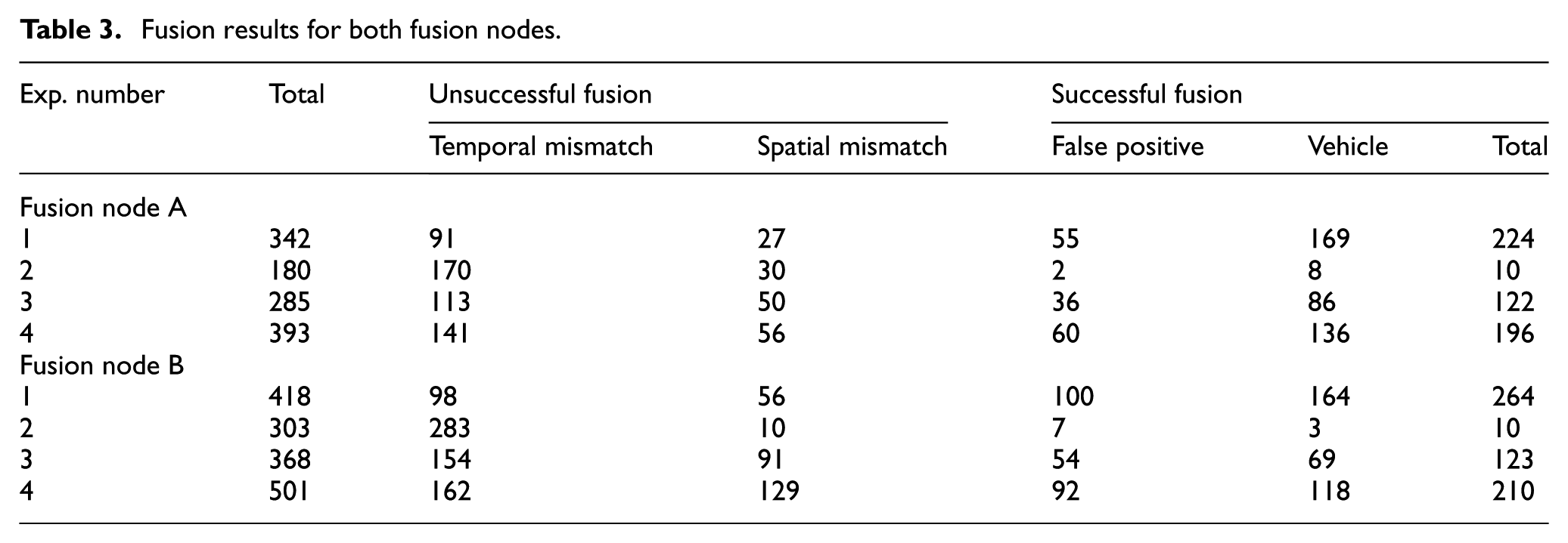
The second goal of experiments was to see how many AoA results individual sensors produce and how many of these lead to successful fusions. Table 2 presents the total number of messages sent to fusion node by all four sensors of a cluster. Each message contains a new AoA value, so the number of messages reflects the total number of valid AoA results produced by sensor nodes. Comparing message send times with the all the times when a vehicle was in the FOV of sensors, reveals that about 40% of messages for cluster A and roughly half of messages for cluster B occur when no vehicle is present (see Table 2). It shows that the environment is noisy and a lot of sound sources are detected, that are not of interest. Fusion helps improve the end result and decrease false positives by applying constraint checking and eliminating for example isolated AoA instances of individual sensors and concurrently produced random AoA instances of multiple sensors. For experiment number 3, the ratio of false positives and correctly detected vehicles improves to 30%/70% for cluster A and 44%/56% for cluster B (consider Table 3 successful fusions). The fact that sensor nodes send AoA messages when there are no vehicles in their FOV and that fusion nodes mostly don’t fuse these results is also evident from the experiment timeline depicted in Figure 12.

The third and final goal was to determine the difference of bandwidth usage between forwarding all sensor messages and forwarding only fusion result messages to the higher ISR level (e.g. an operating military unit and a remote database). In all four experiments, the amount of fusion messages sent was approximately 10 times less than the number of sensor messages sent (see Table 2). However, what is more important than the total amount of messages sent is when they are sent. It is possible to see in Figure 12 that near vehicle occurrence times the number of sensor messages increases (sections of narrow black stripes get denser). This is because all sensors detect the vehicle and want to use (the shared) communication channel at the same time. In our small WSN of eight sensors, this did not cause a problem, not even for experiment number 4, where message sending intervals where changed, such that sensor nodes sent AoA results (when they had any) at an interval of 1 s. While we were able to show that by utilising in-sensor signal processing and in-network fusion it is possible to limit the total number of messages generated by a WSN, we were not able to demonstrate significant packet collisions and congestion of our network at all. An experiment with either a larger number of nodes or shorter message sending intervals is probably needed to demonstrate this.

In conclusion, the four experiments demonstrated the benefit of using in-network distributed data fusion to increase the dependability of WSN results and to decrease the amount of data forwarded to end users. It was also shown that data validity checking (at least against temporal and spatial compatibility) is essential for correct data fusion. We expected to see congestion at network usage peaks, but did not succeed in creating situations where network becomes congested by an overflow of sensor messages. Since the minimum message sending interval of 1 s (see experiment 4) and cluster size of approximately 10 nodes is sufficient and reasonable for our monitoring applications, we do not attempt to find the communication breaking point of the WSN at this moment. In general, the WSN was able to fulfil its task of detecting passing vehicles, although a considerable amount of false positive results were also produced. This shortcoming can further be improved by adding additional sensors to the WSN.

Conclusion

In this article, we have described contemporary situation awareness needs for ISR applications and presented the design and implementation of one possible approach, in the form of a real-life deployed WSN that satisfies those needs. ISR users operate at different levels of military hierarchy and have very different data and information needs depending on the tactical or strategical context. Some need near-real-time sensor information from their vicinity for tactical operation, others need already filtered and fused and/or aggregated information for specific purposes and yet others need matured high level information for strategic decision making and long-term analysis. Such a variety of network users require the creation of information understandable by humans at all hierarchical levels of data production and fusion and in each with their own time and location requirements. In-sensor signal processing (Mist Computing) avoids overwhelming the network with raw data and is the first step to providing data ready to be presented (D2D readiness) for human users.

Our WSN design utilises a middleware-based solution, which supports the service-oriented approach, dynamic data provider discovery and run-time ad hoc (re)formation of network links. It also supports validity checking of communicated data based on temporal and spatial constraints established in service agreements between data providers and consumers. The consistent utilisation of spatial and temporal constraints for ensuring data validity and mutual conformity is essential for correct data fusion and aggregation. Enabling correct in-network fusion in turn improves the quality of information provided by the overall network, helps to eliminate false positives and also reduces considerably bandwidth requirements. Two experiments were described both demonstrating the benefits of pushing computation to the edge of IoT. The first experiment was conducted to evaluate the feasibility of the entire proposed WSN in a military operation scenario and the purpose of the second experiment was to evaluate network communication loads and in-network data fusion efficiency. The WSN experiments demonstrated how data collected by the WSN are dynamically used at the different levels of military operation as dictated by D2D paradigm.