
Abstract
As we know, the degree of freedom approximates the capacity of a network. To improve the achievable degree of freedom in the K-user interference network, we propose a rank minimization interference minimization algorithm. Unlike the existing methods concentrating on the promotion of degree of freedom, our rank optimization method works directly with the interference matrix rather than its projection using the receive beamformers. Moreover, we put the trace constraint of the square root of desired matrix into the rank optimization to prevent the received signal-to-interference-plus-noise ratio from reduction. The decoders are designed through a weight interference leakage minimization method. Considering that the practical obtainable signal-to-noise ratio may be limited, we improve the design of decoders in rank minimization interference minimization, and propose the rank minimization rate maximization. Rank minimization rate maximization aims to reduce the impact of interference on undesired users as much as possible while improving the desired data rate. Simulation results show that rank minimization interference minimization algorithm can provide more interference-free dimensions for desired signals than other rank minimization methods. Rank minimization rate maximization outperforms rank minimization interference minimization at low-to-moderate signal-to-noise ratios, and its performance gets closer to rank minimization interference minimization with the increase in signal-to-noise ratio. Furthermore, in an improper system, rank minimization rate maximization still performs well.
Keywords
Introduction
Interference is regarded as the principle limitation to wireless communication networks. An increasing number of researchers join to study the interference elimination for wireless networks. At present, the most commonly used interference suppression scheme is orthogonal resource allocation. However, when K users share the resources, each user only achieves 1/K of the total resources by orthogonal schemes. As an advanced technique, the concept of interference alignment (IA) has been proposed in Cadambe and Jafar’s 1 paper. The core feature of IA is to divide the received signal space into two subspaces. One is for desired signals and the other is for interfering signals. At the initial stage of research, IA schemes were presented in the closed form expressions such as Cadambe and Jafar, 1 Kim and Torlak, 2 Tresch et al., 3 and Xu et al. 4 However, these closed form solutions were only achieved in certain cases. Besides, it was a tough job to calculate the precoding matrices with the user number increasing.
To overcome this difficulty, researchers provided some iterative methods to solve the aligned problem.5–20 In Gomadam et al., 12 an iterative algorithm called interference leakage minimization was presented for the multi-input, multi-output (MIMO) interference channel (IC), which aimed to minimize the sum of interference power at each receiver. This algorithm was extended to MIMO cellular networks in Zhuang et al. 13 According to Jafar, 15 the degree of freedom (DoF) was based on a high signal-to-noise ratio (SNR) approximation of the network performance. Hence, the promotion of DoF is vital to improve the system performance at high-SNR region. Papailiopoulos and Alexandros, 16 Du and Ratnarajah, 17 Du et al., 18 Rihan et al., 19 and Sridharan and Yu 20 all tried hard to enhance the system DoF. The authors proposed a rank constrained rank minimization (RCRM) scheme in apailiopoulos and Alexandros. 16 RCRM minimized the rank of the interfering signals with full rank constraint on the desired signals. As the nuclear norm is the convex envelope of rank, 21 RCRM introduced the nuclear norm heuristic as convex approximation to obtain the convex solution of optimization problem. Using the same framework, Du and Ratnarajah, 17 Du et al., 18 Rihan et al., 19 and Sridharan and Yu 20 further improved RCRM. A reweighted version of nuclear norm minimization for finding the optimal encoders was presented in Du et al. 18 Compared with RCRM, the literature 19 reduced the running time per iteration. The literature 20 studied the application of RCRM in multi-antenna cellular network. It can be seen that these schemes all take the rank of the interfering signals as the cost function despite that the approximation methods are different. Nevertheless, it is absolutely impossible to realize the perfect IA; thereby, there exists leaked interference at each receiver and the receiver may be severely influenced by this high interference power. Apart from the above schemes, the literature 22 analyzed the achievable DoF over space, time, and frequency. An IA scheme was proposed in Vahdani and Falahati, 23 which attained higher multiplexing gain using a lot lower number of channel extension.
In this article, we first present the rank minimization interference minimization (RMIM) algorithm. Unlike the methods proposed in Jafar, 15 Papailiopoulos and Alexandros 16 , Du and Ratnarajah, 17 and Recht et al., 21 we design the precoders to minimize the sum of the ranks of the interference mapping matrix, where the interference mapping matrix denotes the interference matrix without projection by the decoders. Although the precoders designed by rank optimization methods can largely depress the interference at each undesired receiver, this selfless way cannot guarantee the final interference subspace is far enough from the desired subspace, which could lead to the reduction in signal-to-interference-plus-noise ratio (SINR) at the desired receiver. To alleviate this drawback, we put the desired projection modulus constraint into the rank optimization, where the desired projection modulus is the Frobenius norm of the desired matrix projected into the decoding space. Since the Frobenius norm is convex, we choose the trace of the matrix square root of desired matrix as the final constraint under the restriction of the Hermitian positive definite desired signal matrices. For the decoders’ design in RMIM, we first calculate the decoders using the interference leakage minimization scheme. Since this method does not take the noise statistics into account, we multiply each decoder with a weighted factor, where the weighted factor is a non-negative weight parameter that is determined empirically based on SNR. As the RMIM scheme aims to maximize DoF, it may not be favorable in the low-to-moderate SNR region. Considering the practical obtainable SNR, we improve the RMIM and propose the rank minimization rate maximization (RMRM) approach. The decoders in RMRM are designed to reduce the impact of interference on undesired users as much as possible while improving the desired data rate. As it can be proved that the cost function in RMRM is unitarily invariant in decoders, we utilize the steepest descent method on the Grassmann manifold to find the optimal decoders. To further improve the performance of RMRM in low SNR region, the initial iteration point is chosen to maximize the received SINR. In the simulation, we validate the effectiveness of RMIM that maximizes the achievable DoF. Compared with literature,16,18,19 RMIM compresses the dimensions occupied by interfering signals and provides more interference-free dimensions for the desired signals. RMRM improves the performance of RMIM in low-to-moderate SNR region, and with the increase in SNR, the system sum rate achieved by RMRM gets closer to RMIM. Simulation results also show that for an improper system, the average sum rate achieved by RMRM does not degrade compared to that of reweighted rank constrained rank minimization (RRCRM).
The rest of this article is organized as follows. Section “System model” introduces the system model. The methods of RMIM and RMRM are described in section “RMIM and RMRM,” respectively. Section “Simulation results and analysis” provides the results of simulation analysis. Finally, we conclude the article in section “Conclusion.”
System model
Consider a static flat-fading K-user MIMO interference system, where all the transmitters send their data synchronously. Each transmitter is equipped with

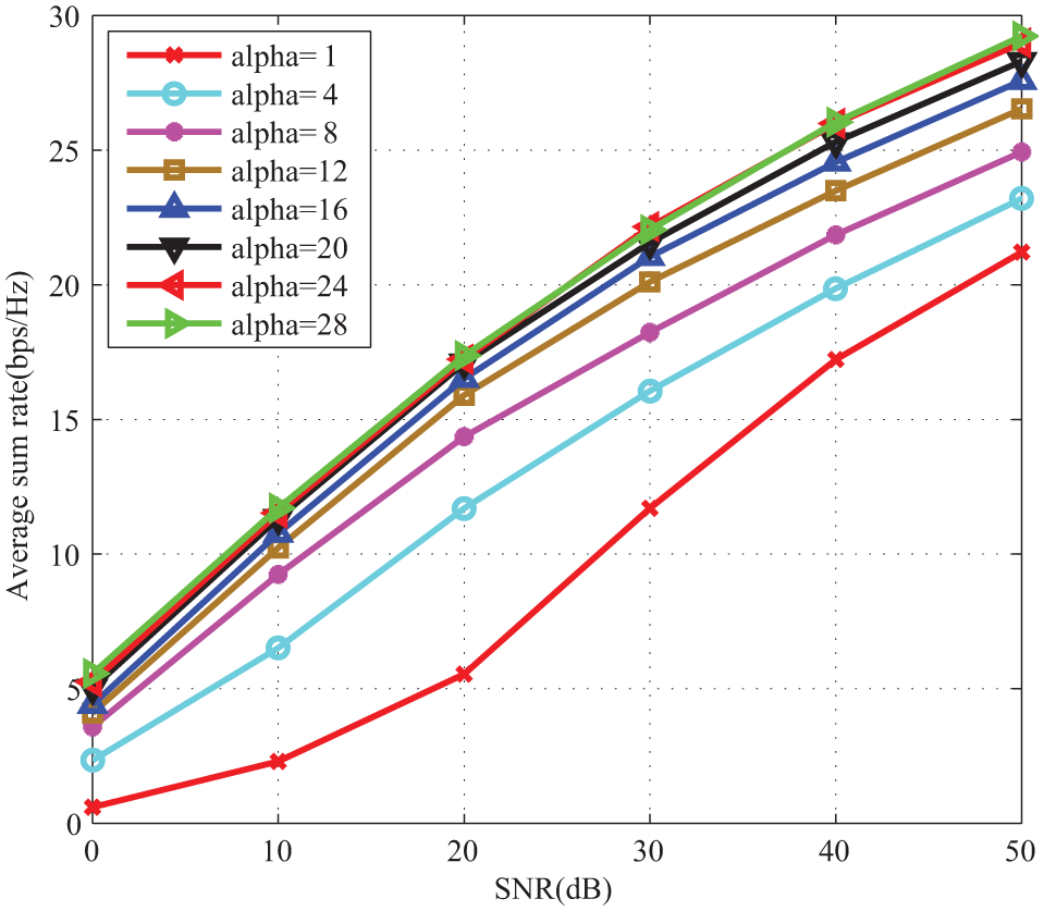
System model of K-user interference alignment.
The received signal at receiver k is given by
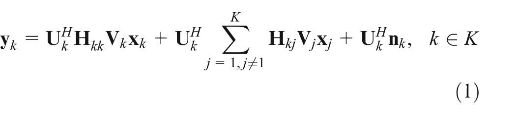
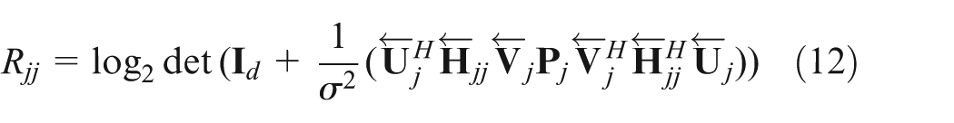
where

On the reciprocal channel, we assume that
RMIM and RMRM
Precoding matrix design
For simplification, we define
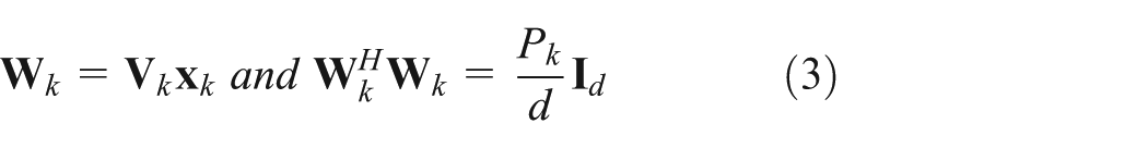
Figure 2 shows the perfect IA. Ideally, all the interfering signals can be aligned in the same subspace and the decoding space is the space orthogonal to the interfering subspace. However, as seen in Figure 3, not all the interfering signals can be aligned with

Perfect interference alignment.

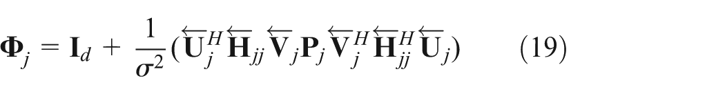
Practical interference alignment.
We define

The rank of a matrix can describe its column space dimensions, in order to compress the dimensions occupied by interference signals. The precoders design should be based on minimizing the rank of

As the nuclear norm is the convex envelope of rank, the cost function is equivalent to

After the optimal solution is obtained, the distances between different interference subspaces are sufficiently small, that is, all the interference subspaces almost overlap in the same subspace. Although the precoders designed by the above method can largely depress the interference at each desired receiver, this selfless way cannot guarantee the final interference subspace is far enough from the desired subspace, which could lead to the reduction of SINR at the desired receiver. In order to resolve this problem, we put the desired projection modulus constraint in the rank optimization, where desired projection modulus is the Frobenius norm of the desired matrix projected into the decoding space. The constraint can be expressed as

where
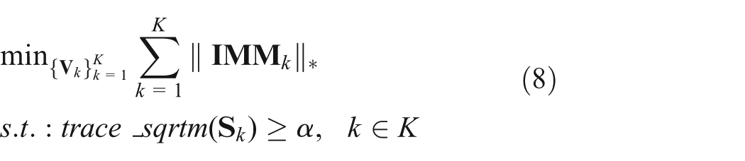
where the desired signal matrix is denoted as
Receive filter design
The receive filter design of RMIM
Obviously, when all the interfering signals align to the same subspace, the decoding space meeting the leakage interference power minimum is the space orthogonal to the aligned space. Thus, we can adopt the interference leakage minimization method 12 to devise the decoders. The leakage interference power can be denoted as
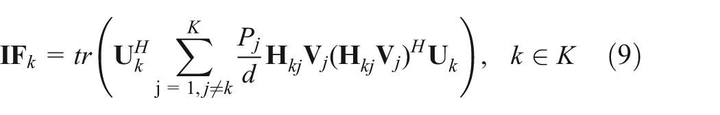

Let

where
The receive filter design of RMRM
Since the precoders and decoders in RMIM are designed to maximize the available DoF, RMIM can guarantee the high data rate in the high-SNR region. Nevertheless, in some scenarios, the practical SNR may be limited. With this in mind, RMRM improves the decoders’ design of RMIM and performs the design procedure under the reciprocal channel. As seen from Figure 1, the signal sent from the transmitter j is useful to the receiver j and useless to receiver


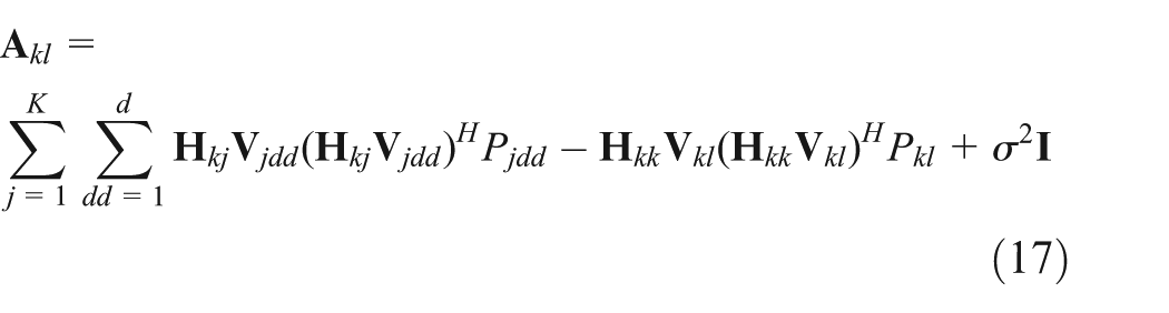
To maximize the single-user data rate at each receiver, we propose a win-win solution. At each transmitter, the win-win scheme is expected to reduce the impact of interference on undesired users as much as possible while improving the desired data rate. Thus, we define the cost function as

where the determinant of matrix is denoted by

As RMRM resorts to performing the design of decoders on the Grassmann manifold, it is necessary to choose a suitable initial point in case that the initialization point influences the eventual outcome. Considering that the data rate actually depends on the received SINR at low-to-moderate SNR, we take the

where
where
Next, we perform the design of
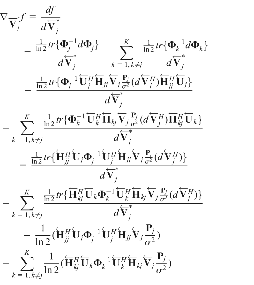
Then, we have

Where

The tangent vector on the Grassmann manifold is denoted as

where
Simulation results and analysis
We consider a three-user IC where each user wishes to achieve d DoF. The system is expressed as
where
We calculate the interference-free dimensions from 0 to 60 dB and then plot the average interference-free dimensions’ results of the seven runs in Figures 4–7. In the four pictures,

System

System

System

System
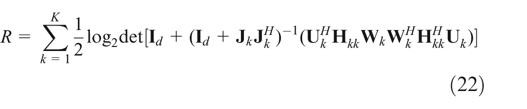
Figures 8 and 9 show the influence of
Comparison of the average sum rate under different

Comparison of the average sum rate under different
Figure 10 shows the average sum rate for

Average sum rate versus SNRs for
Figure 11 illustrates the performance of the average sum rate for
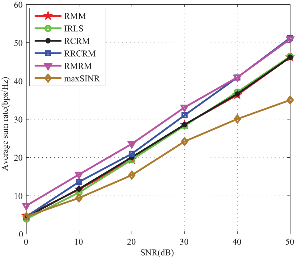
Average sum rate versus SNRs for
The previous figures show the results of performance comparison. One may be concerned by the computational complexity of RMIM and RMRM. To investigate this concern, we present Figure 12, in which the convergence of different schemes versus different iteration numbers is shown. The

Convergence of the alternating algorithms (SNR = 40 dB).
Conclusion
To conclude, in this article, we present two algorithms for IA, RMIM and RMRM. They both adopt the rank minimization method to acquire the optimal precoders. However, they are different at the design of decoders. We work directly with the interference matrix rather than its projection using the decoders which is adopted in other rank minimization methods. In order to prevent the received SINR from reduction, we put the trace constraint of the square root of desired matrix into the rank optimization. In RMIM, the decoders are designed to minimize the leakage interference power. Although RMIM guarantees the high data rate in the high-SNR region, it is not favorable in the low-to-moderate SNR region. In light of this, we improve the RMIM scheme and propose RMRM approach which aims to reduce the impact of interference on undesired users as much as possible while improving the desired data rate. RMRM takes the decoders to maximize the received SINR as the initialization dot on the iterative computing method and finds the optimal decoders utilizing the steepest descent method on the Grassmann manifold. Simulation results show that RMIM provides more interference-free dimensions for the desired signals. The simulations also indicate that RMRM improves the performance of RMIM in low-to-moderate SNR region and has a matched performance with RMIM with increasing SNRs. Moreover, for an improper system, the average sum rate achieved by RMRM does not degrade compared to that of RRCRM.
Footnotes
Appendix 1
In the following, we will prove that the Frobenius norm constraint in equation (7) can be replaced by the trace of the matrix square root of desired signal matrices.
Proof . Using the identity that
where the desired signal matrix is denoted as
Similarly, according to Cauchy inequality
Thus
As the sum of the square roots of
Appendix 2
Suppose
Proof .
Academic Editor: Florentino Fdez-Riverola
Declaration of conflicting interests
The author(s) declared no potential conflicts of interest with respect to the research, authorship, and/or publication of this article.
Funding
The author(s) disclosed receipt of the following financial support for the research, authorship, and/or publication of this article: This article was funded by the National Natural Science Foundation of China (grant no. 51509049), the National key research and development program (2016YFF0102806), the Natural Science Foundation of Heilongjiang Province, China (grant no. F201345), and the Fundamental Research Funds for the Central Universities of China (grant no. GK2080260140).