Sage Journals: Discover world-class research

Abstract

With the popularization of Internet of things, its network security has aroused widespread concern. Anomaly detection is one of the important technologies to protect network security. To meet the needs of automatic and intelligent detection, supervised machine learning is widely used in anomaly detection. However, the existing schemes ignore the problem of data quality, which leads to the unsatisfactory detection effect in practice. Therefore, practitioners may not know which algorithm to choose due to the lack of review and evaluation of anomaly detection methods under low-quality data. To address this problem, we give a detailed review and evaluation of six supervised anomaly detection methods, as well as release the core code of feature extractor for pcap format traffic traces and anomaly detection methods for reuse. We evaluate the methods on two public datasets (one is a simulated network dataset and the other is a real Internet of things dataset). We believe that our work and insights will help practitioners quickly understand and develop anomaly detection schemes for Internet of things and can provide reference for future research.

Keywords

Internet of things security anomaly detection machine learning low-quality data supervised learning

Introduction

With the rapid development of intelligent devices and network technology, the Internet of things (IoT) has been widely applied. Although zero trust security protection protocol has been deployed,¹ IoT still faces many challenges. As the IoT covers whole computer field, it has a wider attack surface. And it is constantly subject to traditional and emerging security threats. Anomaly detection, which aims to mine attack events in the IoT, is an important line of defense for network security. In the IoT, traffic can come at any time, including normal traffic as well as attack traffic, which is often used as data sources to detect network anomalies.

Network traffic–based anomaly detection has become a hot research field in recent years. As an automatic and intelligent technology, machine learning has been widely adopted for anomaly detection in the IoT security field. Many anomaly detection tasks of IoT cyberattacks can be transformed into supervised classification problems.^2–6 The supervised machine learning is an inferring task from labeled training data. In training data, each instance consists of an input object (usually a vector) and a corresponding class value (also called a label). It analyzes the training data and generates an inferred output, which is a map of the input vector. An optimal solution will allow the algorithm to correctly determine the class labels of those newly arriving instances.

A major challenge for training supervised anomaly detection model is the need for high-quality data. The existing work shows superior performance because their data have been carefully processed. In practice, it is difficult to obtain high-quality data. Therefore, their effect may be far from satisfactory when actually deployed. Thus, we find a gap between research in academia and industry. First, to our knowledge, there is a lack of review of anomaly detection framework, methods and principles in the field of IoT. Developers have to take a lot of time to browse a lot of literature to understand the anomaly detection framework. Second, there is a lack of supervised anomaly detection methods for fine-grained comparison under low-quality data. Therefore, developers do not know which anomaly detection method is the most effective in practice.

To bridge this gap, we provide a detailed review and evaluation of supervised classifiers for IoT anomaly detection in the case of low-quality data. Meanwhile, we release the core code of feature extractor and anomaly detection methods. We firmly believe that our work can enable relevant practitioners to quickly start IoT anomaly detection methods and save time for development, as well as our insights can provide guidance for future work.

Specifically, we review six representative supervised anomaly detection methods in recent studies, such as logistic regression (LR),⁷ support vector machine (SVM),⁸ decision tree (DT),⁹ naive Bayes (NB),¹⁰ random forest (RM),² and multi-layer perceptron (MLP).¹¹ We also perform a fine-grained evaluation of these algorithms under low-quality data. We group low-quality data issues into the following three scenarios:

Missing category. Attack and protection are antagonistic and symbiotic. With preventive measures in place, attackers will change to bypass existing protections. As a result, new types of network attacks emerge in an endless stream. Therefore, unlike labeling text or images, some forms of attack do not appear when labeling the data. Thus, there is a lack of labels for evolutionary attacks.

Less labeled data. Data labeling is an extremely expensive task that requires not only expert domain knowledge, but also a lot of manual operations, which generally take a long time to perform. As such, there may be only a small amount of the data labeled manually, that is, low data.

Label assignment error. Due to time constraints or limited expertise, the labels provided may contain errors. For example, different types of attacks may be assigned the same category, normal events are labeled as attack events, and so on.

In summary, we make the following contributions in this article:

We provide a detailed review of commonly used supervised anomaly detection methods for automated IoT traffic anomaly detection.

We release an open-source toolbox for feature extraction and six supervised anomaly detection methods.

We conduct a fine-grained evaluation of benchmarking the effectiveness of anomaly detection methods under low-quality data.

Framework review

Figure 1 illustrates the overall framework for IoT traffic–based anomaly detection. The anomaly detection framework mainly consists of three components: network traffic collection, feature extraction, and anomaly detection.

Figure 1.

Framework of anomaly detection. SVM: support vector machine.

Network traffic collection

Before analyzing network traffic, the acquisition of traffic data is the first step. There are usually two network traffic collection methods, that is, real network traffic collection and simulated network traffic collection.

Real network traffic collection usually uses specific collection software (e.g. Tcpdump¹² or Wireshark¹³) to collect networks running in real environments (such as campus networks, enterprise networks, and IoT networks). Then the captured traffic data are analyzed and labeled for subsequent use. For example, Lopez et al.¹⁴ analyzed and dissected a week’s worth of residential user traffic on a large telecom operator’s fixed broadband Internet access network and obtained an analysis of the security alerts generated by the intrusion detection system. Mirsky et al.¹⁵ collected and analyzed a real Internet protocol (IP) camera video surveillance network. The collected real network traffic data may be unbalanced, thus it needs to take a lot of time for data preprocessing.

Simulated network traffic collection usually constructs the desired target network, and then injects abnormal events by simulating network attacks. For example, Hodo et al.¹⁶ constructed a substation automation network. They simulated the communication between the substation slaves and the server based on the data obtained from the real substation and simulated the behavior of the system under attack. The traffic data collected by simulating the network are relatively balanced, but the simulated attack is also a known abnormal type. In addition, the simulated network traffic does not reflect the real network conditions.

For collected network traffic, a packet is the unit that provides network payload. Packet-based traffic is based on TCP (Transmission Control Protocol), UDP (User Datagram Protocol), and ICMP (Internet Control Message Protocol). Data packets carry a large amount of valuable data for network traffic analysis. Messages are hierarchically divided at the packet level, encapsulated into packets, and paired with addresses and headers, which is a process of encoding. It is then sent to the target address for decoding and execution. File headers guide packets through the network and can be used to identify and filter packets as they flow through the network using information such as IP address, port, and protocol number.

Feature extraction

After capturing network traffic, the next step is feature extraction, which transforms the traffic data into numerical vectors that machine learning can understand. In existing work, feature extraction for network traffic can be divided into two categories: packet-based feature vector and flow-based feature vector.

Packet-based features refer to the statistical features extracted at the traffic packet level, for example, the message length of each packet, the payload length of each packet, the value of TCP window length of each packet, and TCP flags. Nakahara et al.¹⁷ selected the characteristics based on the packet, such as the number of packet and the length of packet, as the feature vectors to train a detection model.

Flow-based features are the feature vectors extracted at the flow level. A flow is defined by a quintuple that includes source IP address, destination IP address, source port, destination port and protocol. Therefore, a flow is a sequence of packets that has the same IP address, port, and protocol. Flow-based features can be flow duration, average number of bytes from server/client in each flow, average number of packets from server/client in each flow, and so on. Hafeez et al.¹⁸ extracted flow-based features to train a deep learning model.

Due to the explosive growth of network traffic, packet-based feature extraction will produce more data, which will affect the operation efficiency of the detection model. Although flow-based feature extraction alleviates the problem of large amount of data to a certain extent, it will lose the detailed information at the packet level. Therefore, a lot of work combines packet-based and flow-based feature extraction. Liu et al.¹⁹ combined them for training and traffic identification. To this end, we also develop a feature extractor for collected traffic in pcap format, which extracts both packet-based and flow-based feature. The statistics include common measurement indicators, such as mean and standard deviation. The flow chart of feature extractor is shown in Figure 2.

Figure 2.

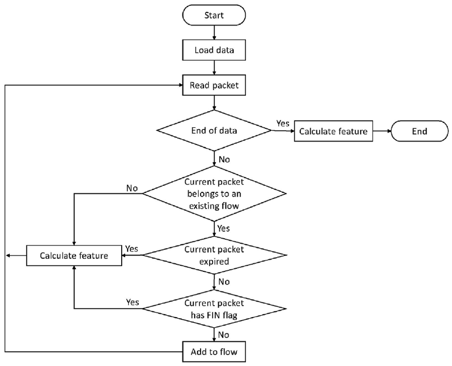
The flow chart of feature extractor. FIN: finished sending data.

The program of feature extractor is as follows. First, the pcap file of network traffic is loaded. Second, read the data packet. If it is not the end of the file, judge whether the current data packet belongs to an existing flow; otherwise, calculate the features and the program ends. Third, if the current packet belongs to an existing flow, judge whether the current packet has expired (e.g. the expired time is set as 30 s); otherwise, calculate the features and continue to read the packet. Fourth, if the current packet has not expired, judge whether the current packet contains a finished sending data (FIN) flag; otherwise, calculate the features and continue to read packet. Fifth, if the current packet does not contain the FIN flag, add the current packet to the existing flow; otherwise, calculate the features and continue to read the next packet. Until the end of file reading.

We write the feature extractor in C language and release the core code on github.²⁰ Readers can optimize on this basis and achieve the features they need for their own datasets.

Anomaly detection

After extracting the numerical feature vector, the machine learning algorithms can be used to train and generate the detection model with optimized parameters. The detection model then can be used to distinguish whether the incoming traffic is abnormal or not.

We will evaluate the performance of supervised machine learning algorithms under low-quality data. The evaluation algorithms will be described in detail in the next section.

Machine learning algorithms

Our goal is to cover a wide range of classification and learning algorithms with different implementation principles and examine their performance under low-quality data. Therefore, we will compare six representative supervised machine learning algorithms: LR, SVM, DT, NB, RM, and MLP.

Logistic regression

LR is one of the most popular algorithms because of its simplicity, effectiveness, and strong interpretability. The LR can be used for some common classification problems, such as spam filtering²¹ and network anomaly detection.⁷

When dealing with anomaly detection problems, LR can simply regard it as judging whether it is “0” or “1.” Training LR is to find the decision boundary, as shown in Figure 3.

Figure 3.

An example of logistic regression.

The principle of LR is shown in Figure 4. It first sums the input feature vectors, and then passes through an activation function called sigmoid (if there is no such step, it is LR), whose definition is shown in equation (1). The output of LR is a probability value between 0 and 1. To predict which category a data belongs to, we can set a threshold (e.g. 0.5). To detect anomalies, the label of a traffic feature vector is abnormal if the output probability of LR is $p > 0.5$

f (x) = \frac{1}{1 + e^{- x}}

(1)

Figure 4.

The principle of logistic regression.

Support vector machine

SVM has been proven to be robust and efficient for many problems.²² In the field of anomaly detection, SVM also solves a decision hyperplane.

From the perspective of linearly separable classification, SVM establishes an optimal decision hyperplane so that the distance between the two types of samples closest to the plane is maximized. Here we briefly review the SVM essential elements.

Consider $m$ separable samples ${(x_{1}, y_{1}), (x_{2}, y_{2}), \dots, (x_{i}, y_{i}), \dots, (x_{m}, y_{m})}$ , where $x_{i}$ denotes the feature vector and $y_{i} = \pm 1$ is the label. The object is that the expected output is 1 or −1 for a new arrival sample. To this end, hyperplane equation (2) is designed to distinguish between two categories

\begin{matrix} w^{⊤} x + b = 0 \end{matrix}

(2)

where $x$ is the input vector, $w$ is the filter vector. Parameter $b$ is the bias term and is a scalar. The distance between the hyperplane and the nearest sample point is called the separation edge, which is represented by $s$ . Thus, the goal of SVM is to find $w$ and $b$ such that $s$ will be maximized. One assumes that

{\begin{matrix} w^{⊤} x + b \geq + 1, if y = + 1 \\ w^{⊤} x + b \leq - 1, if y = - 1 \end{matrix}

(3)

Then the following inequality holds

\begin{matrix} y (w^{⊤} x + b) \geq + 1 \end{matrix}

(4)

According to the principle of structural risk minimization, the optimization becomes a convex optimization problem

\begin{matrix} min_{w} ϕ = \frac{1}{2} w^{⊤} w \end{matrix}

(5)

subject to inequality equation (4). To solve the above constraint optimization problem, Lagrange function is introduced and minimized

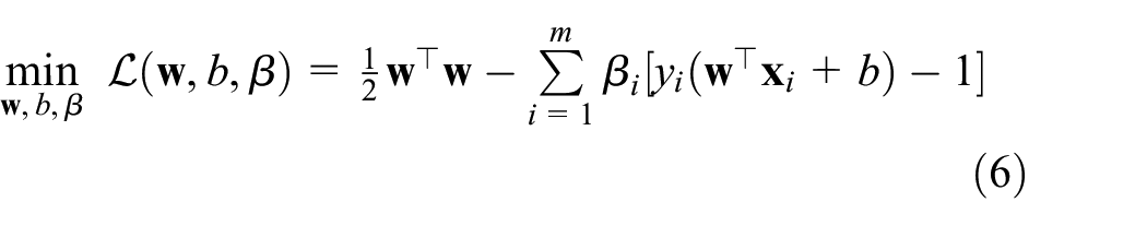
\begin{matrix} min_{w, b, β} L (w, b, β) = \frac{1}{2} w^{⊤} w - \sum_{i = 1}^{m} β_{i} [y_{i} (w^{⊤} x_{i} + b) - 1] \end{matrix}

(6)

After finding the optimal filter $w$ and bias term $b$ , it can be used to predict the new coming network traffic. As shown in Figure 5, the minimum distances of points from different classes to the classification boundary $wx + b = 0$ are equal. Then, those satisfying $wx + b \leq - 1$ are anomaly, and the rest are normal.

Figure 5.

An example of anomaly detection using SVM. SVM: support vector machine.

Decision tree

DT constructs a top–down tree structure by learning a simple decision rule (If… then…, Else… then…) from the feature attributes of the training data. A DT consists of a root node, internal nodes, and leaf nodes. Starting from the root node, the feature with the largest information gain (gini,²³ entropy²⁴) is selected as the division feature. The process is performed recursively until the information gain is small or there are no features to divide.

The leaf nodes represent the decision value, that is, the category labels. Therefore, to judge the state of a traffic feature, you only need to find the final leaf node along the path according to the structure of the tree. And judge whether it is abnormal or not according to the state of the leaf node.

Figure 6 illustrates an example of DT with “gini” criterion, where there are totally 50 samples in the network traffic training data. The “value=[]” in each node means four classes and the corresponding quantity. When dividing the root node, the feature X[23] is selected as the best attribute. Therefore, the whole samples are split into two subsets according to the value of this attribute. The leaf nodes with “gini=0.0” denotes the final label with occurrence number.

Figure 6.

An example of decision tree.

Naive Bayes

NB is a probability classifier that applies the Bayesian formula under the assumption that the features are strongly independent. In the anomaly detection classification work, we assume that the $m$ labels of the category is denoted as $y = {y_{1}, \dots, y_{i}, \dots, y_{m}}$ , $i \in {1, 2, \dots, m}$ , and the $n$ -dimension feature vector is denoted as $x = {x_{1}, \dots, x_{j}, \dots, x_{n}}$ , $j \in {1, 2, \dots, n}$ . According to the Bayesian formula, we can calculate

p (y_{i} | x) = \frac{p (x | y_{i}) p (y_{i})}{p (x)}

(7)

Expanding equation (7), we can get

p (y_{i} | x) = \frac{p ((x_{1}, \dots, x_{j}, \dots, x_{n}) | y_{i}) p (y_{i})}{p ((x_{1}, \dots, x_{j}, \dots, x_{n}))}

(8)

Assuming that the feature attributes $x_{j}$ are independent of each other, equation (8) is converted to

p (y_{i} | x) = \frac{p (x_{1} | y_{i}) \dots p (x_{j} | y_{i}) \dots p (x_{n} | y_{i}) p (y_{i})}{p (x_{1}) \dots p (x_{j}) \dots p (x_{n})}

(9)

Since $p (x_{j} | y_{i})$ , $p (y_{i})$ , and $p (x_{j})$ can be derived from the training data, $p (y_{i} | x)$ can be easily computed.

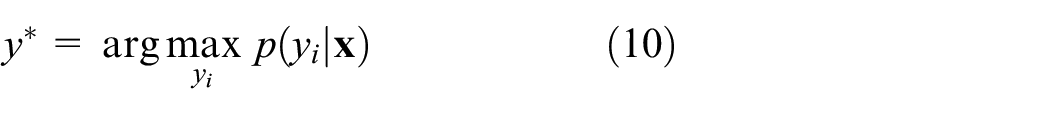
Therefore, the goal of NB classifier is to get the maximum probability in each category, which is the decision result, that is, find $y^{*}$ that,

y^{*} = \arg max_{y_{i}} p (y_{i} | x)

(10)

Random forest

RM uses a random way to build a forest. This forest consists of many DTs. And there is no relationship between each DT in the RM. In anomaly detection field, when a new sample arrives, each DT in the forest predicts which category the sample should belong to, and finally the results of all DTs are combined to get which category the sample belongs to.

As shown in Figure 7, the RM first random samples the training feature vectors (bootstrap samples). When constructing a DT, the best attribute to be split can refer to all or part of the features. Therefore, the input samples of each DT are different. As a result, each tree generated is unique. The advantages of randomness prevent over-fitting, and then finally taking the mean of all DTs for prediction also eliminates some errors.

Figure 7.

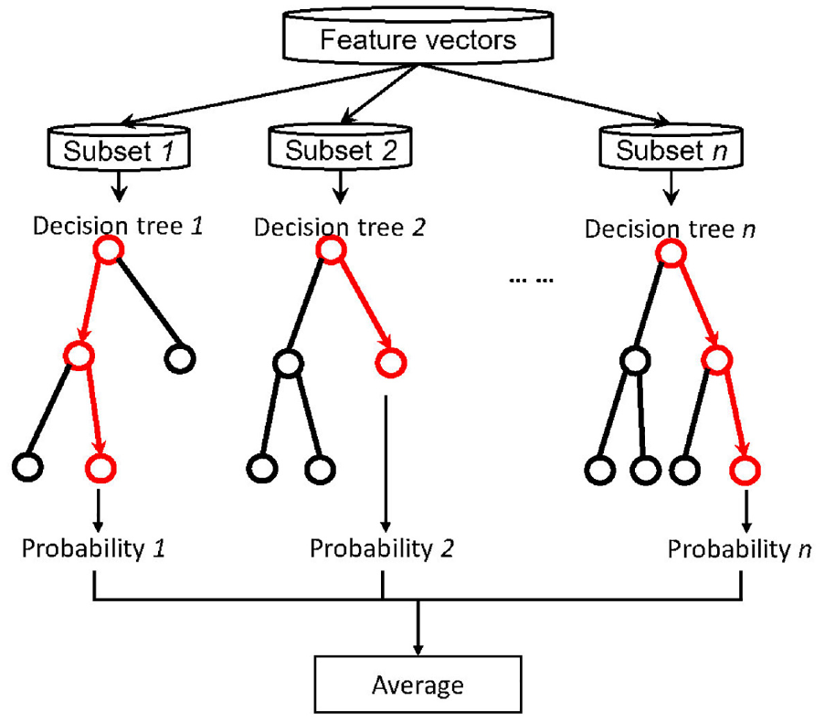
An example of random forest.

Multi-layer perceptron

MLP is a representative of deep learning network. In recent years, it has been widely used in the field of anomaly detection.^25–27

Figure 8 shows a simple MLP network structure. MLP is a multi-layer neural network that can contain multiple hidden layers. Each layer has multiple neurons. Neurons between layers are connected by synapses, and each synapse represents a weight value. In the process of forward propagation, each neuron sums the input data and passes through an activation function (e.g. equation (1)). The output is the probability of different classes.

Figure 8.

A simple example of MLP. MLP: multi-layer perceptron.

Training an MLP requires first building a loss function, which is the mean squared error between the output label and the true label. Training an MLP is the process of discovering the weights that minimize the loss function through back propagation (e.g. using gradient descent).

Evaluation study

In this section, we first introduce the datasets we use and the experiment setup for evaluation. Then we provide the evaluation results of the supervised anomaly detection algorithms under low-quality data.

Datasets

In our evaluation, two public network traffic datasets are used to examine the supervised learning performance under low-quality data:

KDDCup99 dataset is a classical dataset in the network traffic anomaly detection domain. It contains a standard set where a wide variety of attacks are simulated in a military network.²⁸ Among 4,898,431 entries generated, about 80% are abnormal. There are four major types of anomalies, including DoS, U2R (unauthorized access to local superuser privileges by a local unprivileged user), R2L (unauthorized access from a remote machine to a local machine) and Probe (surveillance and probing). In the evaluation, we ignore U2R anomalies due to too few samples. Although the data are outdated, it can provide some insights for future research.

Kitsune network attack dataset is generated on an IoT network,¹⁵ which contains nine different attacks datasets. Each dataset is labeled as malicious (1) or not (0). For convenience, we only use Mirai and OsScan attacks for demonstration.

We randomly choose 80% of dataset as the training data and the remaining 20% as the testing data. To evaluate the performance of algorithms on low-quality data, we adjusted the data to simulate three scenarios:

Scenario 1: Missing Category. To simulate the missing category, we kick out an anomaly in the training dataset, leaving the test dataset unchanged.

Scenario 2: Less labeled data. We randomly select different proportions of the training dataset to form new training subsets.

Scenario 3: Label assignment error. We randomly reverse labels of different proportions in the training dataset.

Experiment setup

We implement the algorithms (LR, SVM, DT, Gaussian NB, RM, and MLP) by utilizing scikit-learn²⁹ and release the code on github.³⁰For the multiple classification tasks, we implement the algorithms with one-versus-rest policy.

We conduct all our experiments on a Linux server, which is configured with 32G memory, 9T hard disk and 16 Intel Xeon E5-2630 central processing units (CPUs).

Metrics

We use the following metrics to report the evaluation results:

Precision: It calculates the proportion of predicted positive instance that are actually positive instance. It is expressed as: $Precision = TP / (TP + FP)$ , where TP denotes true positives and $FP$ denotes false positives.

Recall: It represents the ability of a detection model to identify positive instance, which is defined as: $Recall = TP / (TP + FP)$ , where FN denotes false negatives.

F1-measure: It considers both precision and recall, and is defined as the harmonic average of the two metrics: $F 1 - measure = (2 \times Precision \times Recall) / (Precision + Recall)$

Performance comparison of scenario 1

We first evaluate the performance of machine learning algorithms in the case of missing classes in the training dataset. In practice, lack of attack knowledge is very common, since the attacks are constantly evolving with new types over time. When experts label the data, it is impossible to include all types of attacks.

In this experiment, we kick out the “probe” attack in the training data to deduce the detection model, and then use the well-trained model to test on the testing data with complete categories. Figure 9 shows the results of both algorithms for detecting different events under KDDCup99 dataset. In can be seen that although the training dataset is only lack of probe attack, it will also have a negative impact on the detection performance of all categories.

Figure 9.

Performance in the case of missing DoS under KDDCup99 dataset. (a) Precision for normal. (b) Recall for normal. (c) F1-measure for normal. (d) Precision for DoS. (e) Recall for DoS. (f) F1-measure for DoS. (g) Precision for probe. (h) Recall for probe. (i) F1-measure for probe. (j) Precision for R2L. (k) Recall for R2L. (l) F1-measure for R2L. LR: logistic regression; SVM: support vector machine; DT: decision tree; NB: naive Bayes; RM: random forest; MLP: multi-layer perceptron.

Figure 9(a)–(c) show the detection performance for normal events. We can see that NB shows the worst performance. In the absence of class label information, LR, SVM, RM, and MLP are the most affected, reducing the F1-measure by up to 23%. Figure 9(d)–(f) show the results for detection DoS. Except SVM and DT, other algorithms are very stable. Figure 9(g)–(i) show the performance of detecting probe. Unfortunately, all algorithms cannot detect probe attack. Figure 9(j)–(l) show the detection results of R2L. The results are consistent with detecting normal events, and NB is the worst. The reason is that the data distribution may be different from that of Bayes hypothesis.

Figure 10 shows the results under Kitsune dataset. In the experiment, we use the Mirai attack for training the detection model, and use the OsScan attack as the new unknown attack for testing. We can see that although the detection of the new attack OsScan has a high recall, the precision and F1-measure are far from satisfactory, indicating that the supervised algorithms fail to detect new attacks without new labels.

Insight 1: The emergence of new attacks will reduce the detection performance of the model against known attacks.

Insight 2: The supervised detection model cannot effectively detect unknown attacks.

Figure 10.

Performance in the case of missing DoS under kitsune dataset. (a) Precision. (b) Recall. (c) F1-measure. LR: logistic regression; SVM: support vector machine; DT: decision tree; NB: naive Bayes; RM: random forest; MLP: multi-layer perceptron.

Performance comparison of scenario 2

Unlike labeling images, everyone can do it. Labeling network attacks requires not only professional knowledge, but also a lot of time to complete manually. Therefore, usually only a small part of the data is labeled. In this part, we evaluate the performance under small proportion of labeled data. To achieve this, we randomly sample different proportions (e.g. 0.9, 0.7, 0.5, 0.3) from the training dataset to generate the training subsets. Figure 11 shows the corresponding results.

Figure 11.

Performance in the case of small amount of labeled data under KDDCup99 dataset. (a) Precision for normal. (b) Recall for normal. (c) F1-measure for normal. (d) Precision for DoS. (e) Recall for DoS. (f) F1-measure for DoS. (g) Precision for probe. (h) Recall for probe. (i) F1-measure for probe. (j) Precision for R2L. (k) Recall for R2L. (l) F1-measure for R2L. LR: logistic regression; SVM: support vector machine; DT: decision tree; NB: naive Bayes; RM: random forest; MLP: multi-layer perceptron.

From the whole figure, we can draw two conclusions. First, the performance of all algorithms (e.g. Figure 11(b) and (j)) decreases with the reduction of labeled data. Second, the algorithms fluctuate greatly with the reduction of labeled data, whose robustness is poor. The reason is that the data-driven algorithms can deduce the stable optimal parameters only when there is enough training data.

Figure 12 shows the results of using less training data for kitsune dataset. In terms of F1-measure, DT and RM are more robust than other algorithms. However, their performance still declines with the reduction of the number of training samples.

Insight 3: Insufficient training data lead to the underdetermined parameters of the supervised detection model.

Figure 12.

Performance in the case of small amount of labeled data under kitsune dataset. (a) Precision. (b) Recall. (c) F1-measure. LR: logistic regression; SVM: support vector machine; DT: decision tree; NB: naive Bayes; RM: random forest; MLP: multi-layer perceptron.

Performance comparison of scenario 3

When processing network traffic data, it is very common to have wrong labels. Whether it is real network traffic or simulated network traffic, noise will inevitably be introduced. In addition, the labeling work is completed manually by people, which cannot guarantee that the label is 100% correct.

To simulate the wrong labels, we randomly replace the labels of each category in different proportions (e.g. 2%, 4%, 6%, 8%, 10%) for the training dataset, while the testing dataset remains unchanged. The reported results are shown in Figure 13. Obviously, in the face of label errors, NB is the least robust. Affected by label errors, the performance of DT also decreases. Other algorithms have strong robustness with respect to label errors.

Figure 13.

Performance in the case of wrong labels under KDDCup99 dataset. (a) Precision for normal. (b) Recall for normal. (c) F1-measure for normal. (d) Precision for DoS. (e) Recall for DoS. (f) F1-measure for DoS. (g) Precision for probe. (h) Recall for probe. (i) F1-measure for probe. (j) Precision for R2L. (k) Recall for R2L. (l) F1-measure for R2L. LR: logistic regression; SVM: support vector machine; DT: decision tree; NB: naive Bayes; RM: random forest; MLP: multi-layer perceptron.

Figure 14 shows the results of label errors for kitsune dataset. RM shows the best performance among all algorithms. DT and NB are the least robust.

Insight 4: Label errors also decrease the detection performance of the supervised detection model.

Figure 14.

Performance in the case of wrong labels under kitsune dataset. (a) Precision. (b) Recall. (c) F1-measure. LR: logistic regression; SVM: support vector machine; DT: decision tree; NB: naive Bayes; RM: random forest; MLP: multi-layer perceptron.

Related work

Machine learning is a promising tool for automated and intelligent network traffic anomaly detection. Palmieri³¹ effectively classified the previously unseen total traffic or single traffic as “normal” or “abnormal” traffic through LR. Abbasi et al.⁷ used LR and artificial neural network to extract features and classify the IoT anomalies. The results show that using LR, the classification efficiency and accuracy are higher. Lei,³² Ma et al.,³³ and Davahli et al.⁸ used SVM for network traffic anomaly detection problem. On each cluster of network traffic clustering, Muniyandi et al.³⁴ used the DT to learn the subgroups to refine the decision boundary. Ferrag et al.⁹ used different classifier methods based on DT and rule-based concept to detect Internet of things attacks. Onah et al.¹⁰ adopted NB for anomaly detection in fog computing. Alrashdi et al.² proposed an intelligent anomaly detection system for smart city based on RM. Niandong et al.³⁵ proposed a detection method of RM classification for power network anomaly detection. Teoh et al.²⁶ used the most advanced deep learning technology (e.g. MLP) for cyber security threads detection. Reddy et al.¹¹ uses dense stochastic neural network method to distinguish and classify abnormal behavior and normal behavior according to the types of attacks in the Internet of things.

A lot of work has been done to compare machine learning algorithms in the field of network security. Williams et al.³⁶ showed the impact of feature set reduction using consistency-based and correlation-based feature selection on the performance of NB, C4.5 DT, Bayes network, and NB tree algorithms. They also found that when the classification accuracy is similar, the computational performance is the difference. Anderson and McGrew³⁷ compared six machine learning for encrypted traffic. They focused on the impact of feature extraction on performance of algorithms and conduct coarse-grained testing on the impact of noisy labels. Different from the above work, we divided the data quality in fine-grained evaluation and studied their impact on machine learning algorithms so as to provide insights for future work.

Conclusion

Network traffic is widely used as a data source for IoT anomaly detection. In recent years, network traffic has exploded. To realize automation and intelligence, supervised machine learning technology is widely adopted in anomaly detection. Data quality is a key challenge for supervised machine learning. Practitioners do not know how to select the appropriate algorithm, because there is a lack of reviewing and comparing the performance of these methods under low-quality data. To bridge this gap, we provide a detailed review and algorithm evaluation. We test these methods on two public datasets in fine granularity and released the core code of feature extraction and anomaly detection methods for reuse, which avoids redesign and saves development time.

Footnotes

Handling Editor: Peio Lopez Iturri

Declaration of conflicting interests

The author(s) declared no potential conflicts of interest with respect to the research, authorship, and/or publication of this article.

Funding

The author(s) disclosed receipt of the following financial support for the research, authorship, and/or publication of this article: This paper is supported by the National Key R&D Program of China through project 2020YFB1005600; the Natural Science Foundation of China through projects U21A20467, 61932011, and 61972019; the Beijing Natural Science Foundation through project M21031; and the Populus euphratica found CCF-HuaweiBC2021009.

ORCID iD

Shangbin Han

References

Meng

Huang

, et al. A continuous authentication protocol without trust authority for zero trust architecture. Chin Commun 2022; 19(8): 198–213.

Alrashdi

Alqazzaz

Aloufi

, et al. AD-IoT: anomaly detection of IoT cyberattacks in smart city using machine learning. In: Proceedings of the 2019 IEEE 9th annual computing and communication workshop and conference (CCWC), Las Vegas, NV, 7–9 January 2019, pp.305–310. New York: IEEE.

Tama

Rhee

KH.

An integration of PSO-based feature selection and random forest for anomaly detection in IoT network. MATEC Web Conf 2018; 159: 01053.

Hasan

Islam

Zarif

MII

, et al. Attack and anomaly detection in IoT sensors in IoT sites using machine learning approaches. Intern Things 2019; 7: 100059.

Amangele

Reed

Al-Naday

, et al. Hierarchical machine learning for IoT anomaly detection in SDN. In: Proceedings of the 2019 international conference on information technologies (InfoTech), Varna, 19–20 September2019, pp.1–4. New York: IEEE.

Nawir

Amir

Yaakob

, et al. Effective and efficient network anomaly detection system using machine learning algorithm. Bull Electr Eng Inform 2019; 8(1): 46–51.

Abbasi

Naderan

Alavi

. Anomaly detection in Internet of Things using feature selection and classification based on Logistic Regression and Artificial Neural Network on N-BaIoT dataset. In: Proceedings of the 2021 5th international conference on internet of things and applications (IoT), Isfahan, Iran, 19–20 May2021, pp.1–7. New York: IEEE.

Davahli

Shamsi

Abaei

A lightweight Anomaly detection model using SVM for WSNs in IoT through a hybrid feature selection algorithm based on GA and GWO. J Comput Secur 2020; 7(1): 63–79.

Ferrag

Maglaras

Ahmim

, et al. RDTIDS: rules and decision tree-based intrusion detection system for internet-of-things networks. Fut Intern 2020; 12(3): 44.

10.

Onah

Abdulhamid

Abdullahi

, et al. Genetic Algorithm based feature selection and Naïve Bayes for anomaly detection in fog computing environment. Mach Learn Appl 2021; 6: 100156.

11.

Reddy

Behera

Nayak

, et al. Deep neural network based anomaly detection in Internet of Things network traffic tracking for the applications of future smart cities. Trans Emerg Telecommun Technol 2021; 32(7): e4121.

12.

Jacobson

Leres

MeCanne

Tcpdump: a network monitoring and packet capturing tool, 2001, www.tcpdump.org

13.

Chappell

Combs

Wireshark network analysis: the official Wireshark certified network analyst study guide. Reno, NV: Protocol Analysis Institute, Chappell University, 2010.

14.

Lopez

Silva

Alvarenga

, et al. Collecting and characterizing a real broadband access network traffic dataset. In: Proceedings of the 2017 1st cyber security in networking conference (CSNet), Rio de Janeiro, Brazil, 18–20 October2017, pp.1–8. New York: IEEE.

15.

Mirsky

Doitshman

Elovici

, et al. Kitsune: an ensemble of autoencoders for online network intrusion detection, 2018, https://arxiv.org/abs/1802.09089

16.

Hodo

Grebeniuk

Ruotsalainen

, et al. Anomaly detection for simulated IEC-60870-5-104 traffic. In: Proceedings of the 12th international conference on availability, reliability and security, Reggio Calabria, 29 August–1 September2017, pp.1–7. New York: ACM.

17.

Nakahara

Okui

Kobayashi

, et al. Machine learning based malware traffic detection on IoT devices using summarized packet data. In: Proceedings of the 5th international conference on internet of things, big data and security (IoTBDS), Prague, 7–9 May2020, pp.78–87. Setúbal: SciTePress.

18.

Hafeez

Antikainen

Ding

, et al. IoT-KEEPER: detecting malicious IoT network activity using online traffic analysis at the edge. IEEE Trans Netw Serv Manage 2020; 17(1): 45–59.

19.

Liu

Tian

Zheng

, et al. A distance-based method for building an encrypted malware traffic identification framework. IEEE Access 2019; 7: 100014–100028.

20.

Hans

FlowFeatureExtract, https://github.com/JasonHans/FlowFeatureExtract.git (2022, accessed 25 May 2022).

21.

Dedeturk

Akay

Spam filtering using a logistic regression model trained by an artificial bee colony algorithm. Appl Soft Comput 2020; 91: 106229.

22.

Zhang

Yang

Cui

, et al. Comparison of the ability of ARIMA, WNN and SVM models for drought forecasting in the Sanjiang Plain, China. Nat Resour Res 2020; 29(2): 1447–1464.

23.

Sundhari

SS.

A knowledge discovery using decision tree by Gini coefficient. In: Proceedings of the 2011 international conference on business, engineering and industrial applications, Kuala Lumpur, Malaysia, 5–7 June2011, pp.232–235. New York: IEEE.

24.

Berthold

. Entropy. Best Pract Res Clin Anaesthesiol 2006; 20(1): 101–109.

25.

Lai

Zhou

Lin

, et al. Flow-based anomaly detection using multilayer perceptron in software defined networks. In: Proceedings of the 2019 42nd international convention on information and communication technology, electronics and microelectronics (MIPRO), Opatija, 20–24 May2019, pp.1154–1158. New York: IEEE.

26.

Teoh

Chiew

Franco

, et al. Anomaly detection in cyber security attacks on networks using MLP deep learning. In: Proceedings of the 2018 international conference on smart computing and electronic enterprise (ICSCEE), Shah Alam, Malaysia, 11–12 July2018, pp.1–5. New York: IEEE.

27.

Deore

Kyatham

Narkhede

A novel approach to ensemble MLP and random forest for network security. ITM Web Conf 2020; 32: 03003.

28.

Hettich

Bay

SD.

The UCI KDD Archive, http://kdd.ics.uci.edu (1999, accessed 25 May 2022).

29.

Pedregosa

Varoquaux

Gramfort

, et al. Scikit-learn: machine learning in Python. J Mach Learn Res 2011; 12: 2825–2830.

30.

Hans

MultiClassesAnomalyDetection, https://github.com/JasonHans/MultiClassesAnomalyDetection.git (2022, accessed 25 May 2022).

31.

Palmieri

Network anomaly detection based on logistic regression of nonlinear chaotic invariants. J Netw Comput Appl 2019; 148: 102460.

32.

Lei

. Network anomaly traffic detection algorithm based on SVM. In: Proceedings of the 2017 international conference on robots & intelligent system (ICRIS), Huai An City, China, 15–16 October2017, pp.217–220. New York: IEEE.

33.

Sun

Cui

, et al. A novel model for anomaly detection in network traffic based on kernel support vector machine. Comput Secur 2021; 104: 102215.

34.

Muniyandi

Rajeswari

Rajaram

Network anomaly detection by cascading k-Means clustering and C4.5 decision tree algorithm. Proced Eng 2012; 30: 174–182.

35.

Niandong

Yanqi

Sheng

, et al. Detection of probe flow anomalies using information entropy and random forest method. J Intell Fuzz Syst 2020; 39(1): 433–447.

36.

Williams

Zander

Armitage

A preliminary performance comparison of five machine learning algorithms for practical IP traffic flow classification. ACM SIGCOMM Comput Commun Rev 2006; 36(5): 5–16.

37.

Anderson

McGrew

. Machine learning for encrypted malware traffic classification: accounting for noisy labels and non-stationarity. In: Proceedings of the 23rd ACM SIGKDD international conference on knowledge discovery and data mining, Halifax, NS, Canada, 13–17 August2017, pp.1723–1732. New York: ACM.