Sage Journals: Discover world-class research

Abstract

This study proposes two parameters, including the appearance frequency of harmonics (AFH) and the change in shape of the power spectral density (PSD), which are examined to assess the decline in stiffness of a bridge span. PSDs are obtained from the real vibration signals of the randomized traffic load model based on accelerometer multi-sensors that indicate the change in mechanical behavior of the structure over time. In addition, AFHs evaluate the workability of the structure. With these parameters in mind, actual vibrations in real beam structures are studied with the aim of using structural health monitoring to assess the bearing capacity reduction on Saigon Bridge’s spans. The results show that AFHs and the high-frequency regions relate to the decreased stiffness of the bridge’s spans over a given period of time. In the future, this research can be used to monitor structural health for various types of structure materials and many different bridge spans.

Keywords

Frequency vibration signal power spectral density appearance frequency

Introduction

Currently, the problem of assessing the change of structure by actual measuring signal is done by many studies. This issue is often divided into two trends, including structured method and unstructured method. In each evaluation method, many parameters have been researched and developed. These parameters are summarized as Figure 1.

Figure 1.

Research model from this article.

The damage situation is very complex and complicated in the actual bridge structures, and it is very difficult to detect it accurately. Therefore, the study cannot accurately determine the damage of the real bridge structure (damage location, damage degree, failure time, etc.). The actual load acting on the bridge during its working time is very complicated, and the working environment of the bridge is harsh (high humidity, hot and sunny environment, high abrasion). Therefore, the unstructured method from the article will be much more effective than the current structured method. The article only considers them as a feature that changes the overall stiffness of the structure. This is a new assessment method following current trends. From Figure 1, the change in frequency caused by a fracture does not imply that all of a cracked structure’s inherent frequencies will be altered. The natural frequency value does not decrease, or changes so little, during the monitoring of structural stiffness changes that studies cannot use frequency change as a sensitive parameter in assessing structural change.^1–4 However, a few studies use the natural frequency parameter in determining the defect location in the structure.^5,6 The reason for this is because the damage occurs at a nodal point in the mode form, the measurements will usually show unaltered frequency values. For a simply supported beam, for example, if the third frequency remains fixed, the fracture might appear in two small places on the beam at the spots where the displacement of the third mode shape is zero.

The existence of a fracture is usually associated with a reduction in local stiffness and, as a result, a reduction in natural frequencies. Maguire,⁷ on the other hand, has noticed an increase in natural frequencies as a result of structural degradation. Damage to some pre-stressed concrete beams caused the frequencies to rise, according to the current study. The modulus of elasticity of concrete rose as the pre-stresses reduced, resulting in a rise in frequency. The present research uses natural frequency variation as a feature in the identification of structural defects. The frequency change approach^8–11 has been used to identify cracks in a large number of sheets. Calculating frequency changes from a known sort of damage is a part of several investigations. To detect the existence of damage, the damage is usually theoretically modeled, and the observed frequencies are compared with the projected frequencies.

To detect deterioration, Vandiver¹² looked at the frequency variations in the first two bending modes and the first torsional mode of an offshore light tower. According to numerical study, changes in the effective mass of the tower caused by fluid sloshing in tanks located on its deck would only result in a 1% variation in the frequencies of the three modes under consideration. Vandiver also proved that eliminating most components from the numerical model resulted in variations in resonant frequencies higher than 1%, indicating that damage in most of the components would be visible. Kenley and Dodds¹³ investigated the effects of fractures in a decommissioned offshore plafond on resonance frequencies. Changes in global modal frequencies were shown to be the sole way to identify total severance of a diagonal member. The damage had to produce a 5% change in the overall stiffness before it could be detected, and a 1% change in the resonant frequencies for global modes could be detected.

Pardoen¹⁴ investigated the vibration frequencies and mode forms of a composite beam with a mid-plane delamination. Bending and axial vibrations were examined in four parts of the beam: above, below, and on each side of delamination. The transverse deformations of the sections above and below the delamination were restricted to vibrate simultaneously, allowing the analysis to be performed in the plane of the delamination. To get frequencies and mode shapes, the characteristic equation was numerically solved. Man et al.¹⁵ provided a thorough closed form solution for the frequency of a slotted beam. According to the authors, the smallest slot size visible by their approach is 10% of the beam depth.

To simulate the damage, Choy et al.¹⁶ employed the lower modulus of one or more beam components. The first beam element was considered to be deteriorated, and the modulus associated with this element was changed until the numerical model’s first natural frequency matched the first observed natural frequency. The method was repeated for the second and third natural frequencies, assuming that the damage was located in each of the other constituents. The intersection of flexural rigidity versus element location curves derived from the iterative approach utilizing different natural frequencies yielded the location of the damaged region. Damage at symmetrical sites in a symmetric structure was not distinguishable by the approach.

The ratio of variations in natural frequencies for distinct modes was determined by Hearn and Testa.¹⁷ The damage was determined using the acquired frequency ratios, which were estimated using mode shapes and pre-damaged modal parameters. To identify deterioration in composites, Sanders et al.¹⁸ used Stubbs’ technique in combination with an internal state variable theory. Skjaerbaek et al.¹⁹ investigated a multistory reinforced concrete frame structure and devised a method for detecting deterioration with only one response measurement. Damage was defined as a factor that decreases the stiffness matrix of the substructures that reproduce the structure’s two lowest frequencies.

For the natural frequency analysis of a beam with many fractures, NT Khiem and TV Lien,²⁰ Nguyen et al.^3,8 used a simpler technique. On the basis of the transfer matrix approach and the rotating spring model of a fracture, this was a new method for the natural frequency analysis of a beam with an arbitrary number of cracks. The frequency equation found for a beam with many fractures is universal in terms of boundary conditions, including more realistic (elastic) end supports, and may be built analytically using symbolic codes. The suggested approach is advanced since it does not involve the numerical computation of the high order determinant, which reduces the time required to calculate natural frequencies. The suggested approach is advanced since it does not involve the numerical computation of the high order determinant, resulting in a considerable reduction in the time required to calculate natural frequencies. The influence of each fracture, the number of cracks, and the boundary conditions on the natural frequencies of the beam has been calculated numerically.

JK Sinha et al.²¹ applied beam components with minor changes to the local flexibility in the fractures’ proximity. The fracture locations and diameters are then estimated using this crack model, which is updated to minimize the discrepancy between measured and anticipated natural frequencies. The technique is unusual in that the reduced crack model can immediately assess the location and degree of damage. The reduced crack model may also be used to produce training data for health-monitoring algorithms that employ pattern recognition. The suggested approach has been demonstrated on a beam using experimental data. Many approaches for determining the development of cracks have been proposed in the preceding study. These approaches, however, have a low efficiency. Because the changes in frequency or mode shape are so minor, they are not beneficial in practice.

The natural frequency value is not extremely sensitive to structural changes, as indicated by the preceding research. The shift in the appearance frequency of natural frequencies and the change in the form of the power spectrum are two new discoveries made in the article as shown in Figure 2. The Saigon Bridge, Ho Chi Minh City’s largest bridge, was used to follow the findings of this text over a lengthy period of time. Using measurements from sensors at the bridge, the article evaluates the change of the structure through two new observations. Proposals from this study are shown in Figure 2 in which the research model from the draft proposes to use the power spectral density and the harmonic fundamental frequencies through the vibration signal from the accelerometer milti-sensor system. The results from the article suggest that these are two parameters sensitive enough to be able to assess structural changes over time.

Figure 2.

Research model proposed through this study.

Theory background

The theoretical model used in this study includes four steps as shown in Figure 3:

Step 1: Convert the vibrating acceleration signal from the time domain to the frequency domain by Fourier transform.

Step 2: Build the representative power density spectrum (RPDS) model from the power density spectrum (PSD) model through step 1.

Step 3: Proposed the harmonic fundamental frequencies (AFH) model to determine the change of frequency harmonics.

Step 4: Determine the change of the actual bridge structure by selected features.

Figure 3.

The theoretical model proposed through this study.

Fourier transform and frequency spectrum

A Fourier series is a set of sine and cosine terms that may be used to define almost any function. The Fourier series coefficients define the amplitudes of the sine and cosine terms, each with its own frequency. A strategy for decomposing a recorded dynamic signal into its amplitude and frequency components has recently been presented in Nguyen²² and Ngo et al.²³ The dynamic portion of a signal of an arbitrary period T can be described in equation (1)

A_{n} = \frac{2}{T} \int_{- \frac{T}{2}}^{\frac{T}{2}} y (t) \cos n ω t . dt; B_{n} = \frac{2}{T} \int_{- \frac{T}{2}}^{\frac{T}{2}} y (t) \sin n ω t . dt

(1)

The nth frequency of a Fourier series corresponds to the amplitudes A_n and B_n. The Fourier series becomes an integral in the limit as T approaches infinity. The distance between frequency components shrinks to infinity. As a result, the coefficients A_n and B_n become continuous frequency functions that may be written as A(f) and B(f), respectively.

The Fourier transform analysis^24–26 is expressed as equation (2)

Y (f) = \int_{- \infty}^{\infty} y (t) e^{- i 2 π ft} . dt

(2)

The Fourier transform of y(t) is given by equation (4). The Fourier transform, Y(f), is significant because it depicts the signal as a frequency continuous function. If y(t) is known, then Y(f) will reveal the signal’s amplitude-frequency qualities, which are otherwise hidden in its time base form. If Y(f) is known or measured, we may use equation (4) to reconstruct the signal y(t) equation (3)

Y (f) = \frac{1}{2 π} \int_{- \infty}^{\infty} y (t) e^{- i 2 π ft} . df

(3)

The inverse Fourier transform of y(t) is described by equation (3). It implies that we can recreate the original signal y(t) using the amplitude-frequency features of a original signal. A complex number with a magnitude and phase is known as the Fourier transform as equation (4)

Y (f) = | Y (f) | e^{i ϕ (f)} = A (f) - iB (f)

(4)

Power spectral density concepts

Power spectral density

We now turn to the frequency composition of a naturally occurring random process.^27,28 Because the time history y(t) of the sample function is not periodic, it cannot be represented by a discrete Fourier series. Also, for a stationary process, y(t) goes on forever, and this condition is shown in equation (5).

\int_{- \infty}^{\infty} | y (t) | dt < \infty

(5)

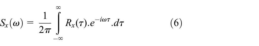
The classical theory of Fourier analysis cannot be applied to the sample function. The Fourier transform of R_x(τ) as given by equation (6):

S_{x} (ω) = \frac{1}{2 π} \int_{- \infty}^{\infty} R_{x} (τ) . e^{- i ω τ} . d τ

(6)

Response power spectral density

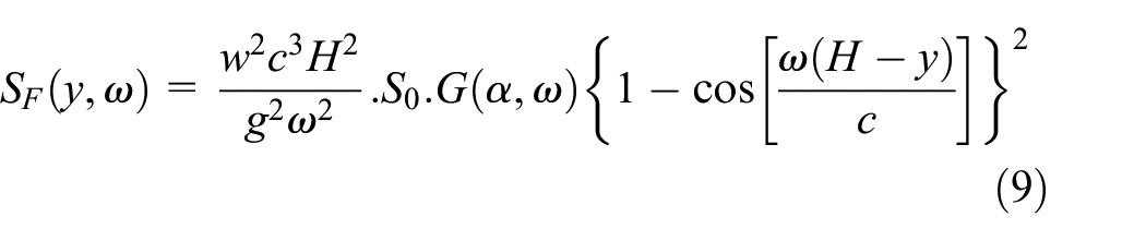
The stationary response PSD is S_p(y, ω) as shown in equation (8), S_F(y, ω) as interpreted in equation (9), and S_M(y, ω) as described in equation (10) for pressure, shear, and moment, respectively.^29,30 They can be readily determined by the following well-known relation given by equation (7)

S (y, ω) = H (y, ω) . H^{*} (y, ω) . S_{0}

(7)

thus

S_{p} (y, ω) = \frac{w^{2} H^{2}}{g^{2}} . S_{0} . G (α, ω) . \sin^{2} [\frac{ω (H - y)}{c}]

(8)

S_{F} (y, ω) = \frac{w^{2} c^{3} H^{2}}{g^{2} ω^{2}} . S_{0} . G (α, ω) {1 - \cos [\frac{ω (H - y)}{c}]}^{2}

(9)

\begin{matrix} S_{M} (y, ω) = \frac{w^{2} c^{3} H^{2}}{g^{2} ω^{2}} . S_{0} . G (α, ω) \\ {\frac{ω (H - y)}{c} - \sin [\frac{ω (H - y)}{c}]}^{2} \end{matrix}

(10)

where

\begin{matrix} G (α, ω) = {(\frac{c}{ω H})}^{2} \\ [\frac{{(1 + α)}^{2}}{{(1 + α)}^{2} \cos^{2} (\frac{c}{ω H}) + {(1 - α)}^{2} \sin^{2} (\frac{c}{ω H})}] \end{matrix}

(11)

Probability density of the peaks

Because most buildings are constructed to handle maximum or peak loads, examining all of the peak values of a random process y(t) and calculating the probability density function among the peaks is beneficial.^31–34 The probability of a peak with a magnitude between z and z+dz among a population of peaks may then be calculated by

p (z) dz ≅ \frac{E [n_{pz}]}{E (n_{p})}

(12)

in which n_pz in the equation is approximately equal to the difference between the number of up-crossings of the level z per unit time n_cz and that of the level z+dz per unit time n_{c, z}₊_dz.

Thus

E [n_{pz}] = E [n_{cz} - n_{c, z + dz}]

(13)

Similarly, E[n_p] is approximately equal to the average time rate of zero up-crossings v₀⁺. Therefore

p (z) dz = \frac{v_{z}^{+} - v_{z + dz}^{+}}{v_{0}^{+}} = \frac{- {dv}_{z}^{+}}{v_{0}^{+}}

(14)

Recall that for y(t) and $\overset{•}{y} (t)$ with uncorrelated Gaussian distribution and zero means, the average time rate of zero up-crossings v₀⁺and z level up-crossings are, respectively

\begin{matrix} v_{0}^{+} = \frac{σ_{\overset{\cdot}{x}}}{2 π σ_{x}}; v_{z}^{+} = \frac{σ_{\overset{\cdot}{x}}}{2 π σ_{x}} \exp (\frac{- z^{2}}{2 σ_{x}^{2}} \end{matrix}); p (z) = \frac{z}{σ_{x}^{2}} \exp (- \frac{z^{2}}{2 σ_{x}^{2}})

(15)

Experimental model

Measurement organizations

Bridge deterioration develops over time, as can be observed. Various metrics were used to assess the vibration signal. The goal of this research is to use vibration signal characteristics to determine changes in bridge degradation over time. The findings of the Saigon Bridge research in Ho Chi Minh City will be given in this report. As seen in Figure 4, the Saigon Bridge connects Ho Chi Minh City’s urban and suburban neighborhoods. It has 32 spans, including three middle spans consisting of structural reinforced concrete bearing beams (the 17th, 18th, and 19th spans). The remaining spans are 24.7 m long and 24 m wide, and are composed of reinforced concrete. Between Ho Chi Minh City and the southern regions, this is the most essential bridge. The measurements are carried out at various times of the day and with varying real traffic loads. To collect and receive data, we employed accelerometer sensors, one of which is depicted in Figure 5.

Figure 4.

View of Saigon Bridge in Ho Chi Minh City.³⁵

Figure 5.

The accelerometer sensor used in the project.

In Tables 1 and 2, it can see that for the first four measurements, the time between adjacent campaigns was approximately 3 months. The time between the 4th and 5th campaigns was 11 months, while it was 27 months between the 5th and 6th campaigns. The process of data acquisition by accelerometer sensors at Saigon Bridge is shown in Figure 6.

Table 1.

Measurement sensor.

Sensor: Vibration accelerometer sensor (SENSR)	Process#: 224
Instrument: SENSR GP 1P	General accuracy: ± (50 mg ± 5% of reading)
Serial#: 1999	Measurement locations: midpoint of each span
Manufacturer: Reference LLC/sensor	Sampling speed: 100 Hz
Number of samples: 2000 samples per files and 30 files at each position
External stimulation: traffic loads from 2011 to 2015 with six measurement campaigns

Table 2.

Time of measurement campaigns.

Campaign	1	2	3	4	5	6
Time	11/2011	02/2012	05/2012	08/2012	07/2013	10/2015

Figure 6.

Measuring at the 1/2 point of the 19th span of Saigon Bridge in Ho Chi Minh City.

Data processing process

The objective of this research is to contribute to the management and assessment of the conditions of bridges that contributed to the development of society. Therefore, the research group has conducted surveys and measurements with vibration accelerometer sensors of some actual bridges in a relatively a little over 5 years as shown in Figure 7.

Figure 7.

Data processing process in this study.

This survey examined the possibility of the application of vibration signal processing methods in the circulation process, and in the assessment of results as well. The signal time and the vibration signal of the bridge will be collected in all circumstances during actual traffic, as long as the actual vibration signals are higher than the interference signal. Figure 8 shows a process to make recommendations for AFH parameters.

Figure 8.

Data processing process of RPDS and the appearance frequency of AFH.

The actual vibration signal processing results from the article are shown as Figure 9.

Figure 9.

The actual PSD of a span structure.

Conclusions of the PSD of real vibration signals

Characteristics of the actual power density spectrum

Measurements of the vibration signals from the actual loads on Saigon Bridge were taken continuously, and these signal measurements are shown in Figure 10. During the actual bridge operation, there are various traffic circulations with different loads and velocities at the same time. So the figures of actual signals will create a set of variable values between the amplitude and the duration to obtain the signals.

Figure 10.

The acceleration vibration signal at one span in Saigon Bridge.

From each data set of real vibration signals at the bridge, we can build a PSD based on the Fourier analysis theory, and it can be shown as in Figure 11.

Figure 11.

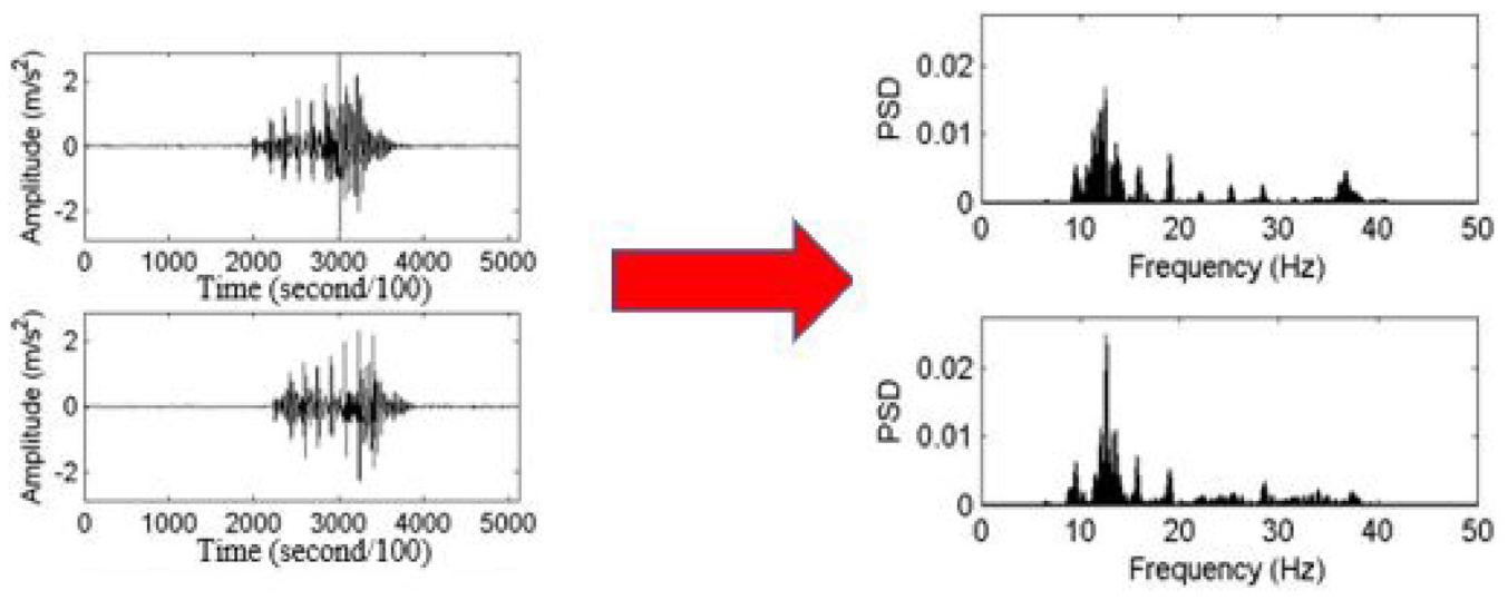
Fourier analysis of the acceleration vibration signal at one span in Saigon Bridge.

Through Fourier analysis, Figure 10 can be transformed from the real vibration signals into PSDs as Figure 12.

Figure 12.

The PSD of the vibration signal of one span in Saigon Bridge.

As Figure 12 shows, it can be seen that the change in circulation during the measurement time can change PSD of the Saigon Bridge span in relatively diverse ways. We made exhaustive determinations of changes in the characteristics of PSD of the Saigon Bridge over 10 consecutive years. The article draws the following conclusions on PSD changes in characteristics as follows:

There are six PSDs, approximately 20% of the survey PSDs total, in which, all harmonics appear only in one resonance region with frequency values at 3–6 Hz. So, the article defines only a single fundamental frequency that is the harmonic frequency with the highest amplitude, and this mean shows that PSD portion of the span will be similar to the free vibrational state of the bridge. However, the graphs of PSD in Figure 13 can clearly show that this frequency value in each graph of PSD is not completely overlapped and shows little deviation (negligible). The small deviation can be explained by the impact of interference signals and errors in the measurement process or data processing.

There are 10 PSDs, approximately 37% of the survey PSDs total, in which, all harmonics are focused mainly on two resonance regions at 3–6 Hz and 10–12 Hz as shown in Figure 12. This mean shows that it is not only the fundamental frequency, approximately 20% of the survey PSDs total in 3–6 Hz of the free vibration state manifesting at the span but also the other frequency in the resonance region between 10 and 12 Hz.

There are 14 PSDs, approximately 43% of the survey PSDs total, such that portions of the PSD show harmonics stretch in 2–24 Hz.

Figure 13.

The representative PSD of one span in Saigon Bridge (a) The representative PSD of 3th span in Saigon Bridge. (b) The representative PSD of 4th span in Saigon Bridge.

The appearance frequency

To assess the possibility of the appearance of the frequencies, we determine the percentage frequency of occurrences of the harmonic, in which the number of the lowest harmonic frequency will always be the highest ratio, and this ratio will descend to the next frequency. Over time, the highest frequency will decline but not the occurrences, and all of its energy will be transferred to the next frequency (priority for the next highest frequency). The entire process of decline in the frequency of occurrence of the fundamental frequencies is captured by Figure 14. The excitation sources are very complex, and the vibrations of higher-order modes are very easy to be excited. The study also claims that it is in fact possible to obtain more than four eigen frequencies or less. However, the frequency limitations of the measuring device (simple, inexpensive, large number, easy to use, etc.) do not measure natural frequencies higher than the fourth order. Therefore, this whole study only investigated the 4th natural frequency as in the article.

Figure 14.

The appearance frequency of the resonance.

The surveying of the value of the fundamental frequencies and appearance frequency of the harmonic fundamental frequencies at the eighth span of Saigon Bridge at different measurement times is shown in Table 3. We can see that the lowest fundamental frequency f₁ = 3.5 Hz has a frequency of appearance to increase with time when the Saigon Bridge was monitored by the research team, and the results were shown in Figure 15(a). Higher frequencies such as f₂ = 5.8 Hz and f₃ = 11.7 Hz declined with time such that the higher the fundamental frequencies, the more the decline compared with other fundamental frequencies as see in Figure 16, as shown in Figure 15(b) and (c). The appearance frequency of f₄ = 17.5 Hz was especially not due to occurrences from the third to the seventh times, as shown in Figure 15(d).

Table 3.

The value and probability of presence of the natural frequencies in the eighth span, Saigon Bridge.

Time	Value of fundamental frequency
	Value	The appearancefrequency of presence
First	f₁ = 3.5 Hz	40%
	f₂ = 5.8 Hz	80%
	f₃ = 11.7 Hz	60%
	f₄ = 17.5 Hz	60%
Second	f₁ = 3.5 Hz	60%
	f₂ = 5.8 Hz	60%
	f₃ = 11.7 Hz	60%
	f₄ = 17.5 Hz	30%
Third	f₁ = 3.5 Hz	60%
	f₂ = 5.8 Hz	60%
	f₃ = 11.7 Hz	40%
	f₄ = 17.5 Hz	10%
Fourth	f₁ = 3.5 Hz	62.5%
	f₂ = 5.8 Hz	50%
	f₃ = 11.7 Hz	37.5%
	f₄ = 17.5 Hz	0%
Fifth	f₁ = 3.5 Hz	70.56%
	f₂ = 5.8 Hz	53.33%
	f₃ = 11.7 Hz	33.33%
	f₄ = 17.5 Hz	0%
Sixth	f₁ = 3.5 Hz	75.14%
	f ₂ = 5.8 Hz	57.14%
	f₃ = 11.7 Hz	28.57%
	f₄ = 17.5 Hz	0%
Seventh	f₁ = 3.5 Hz	81.17%
	f₂ = 5.8 Hz	47.05%
	f₃ = 11.7 Hz	20.28%
	f₄ = 17.5 Hz	0%

Figure 15.

The change of the appearance frequency of presence at eighth span in Saigon Bridge (a) The change of the appearance frequency of presence at 8th span in Saigon Bridge based on the first fundamental frequency. (b) The change of the appearance frequency of presence at 8th span in Saigon Bridge based on the second fundamental frequency. (c) The change of the appearance frequency of presence at 8th span in Saigon Bridge based on the third fundamental frequency. (d) The change of the appearance frequency of presence at 8th span in Saigon Bridge based on the fourth fundamental frequency.

Figure 16.

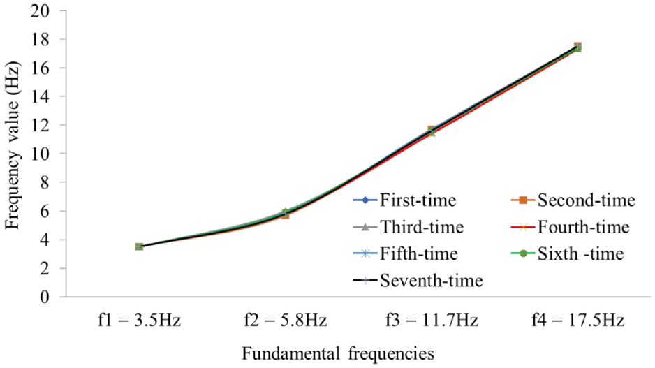
The value of fundamental frequencies at eighth span in Saigon Bridge.

This appearance frequency of presence can also be changed when we compare the time before and after the bridge was repaired. Table 4 is a result of two different times of measuring at the eighth span in Saigon Bridge between the time before repairs on 13 July 2012, and after repairs on 9 December 2012. These changes in the appearance frequencies of the fundamental frequency are shown in Figure 17(a) and (b).

Table 4.

The value and appearance frequency of presence in the fundamental frequencies between the time before repairs on 13 July 2012 and after repairs on 9 December 2012, at the eighth span in Saigon Bridge.

Batch	Value of frequency
	Value	The appearance frequency of presence
Before repairs on 13 July 2012	f₁ = 3.5 Hz	60%
	f₂ = 5.8 Hz	60%
	f₃ = 11.7 Hz	0%
	f₄ = 17.5 Hz	0%
After repairs on9 December2012	f₁ = 3.5 Hz	66%
	f₂ = 5.8 Hz	80%
	f₃ = 11.7 Hz	65.5%
	f₄ = 17.5 Hz	60%

Figure 17.

(a) The change of the appearance frequency of presence at the eighth span in Saigon Bridge between the time before repairs on 13 July 2012, and after repairs on 9 December 2012 and (b) the value of the fundamental frequencies at the eighth span in Saigon Bridge between the time before repairs on 13 July 2012, and after repairs on 9 December 2012.

The change in the shape of the power spectral density

The conclusions show that the lowest resonance region always appears in all of the real PSDs, although the frequency value of this region is smaller than other regions. From this, we can understand that the frequency value of the lowest resonance region is more stable than other regions (the higher value regions). According to the total number of PSDs of the first survey on the Saigon Bridge, the results of this survey show that, for the fundamental frequency located in the highest amplitude of harmonic frequency in PSD that was always surrounded by the resonance regions, the main differences between the real fundamental frequency value and PSD’s fundamental frequency value may be determined by the interference, measurement error, and data processing. The span’s PSD may be displayed in Figure 18 as a result of a survey of the span of the Saigon Bridge with prestressed concrete material at six distinct measurement times (over 5 years). PSDs generated three resonance zones with considerable amplitudes, with the first ranging from 0 to 8 Hz, the second from 8 to 14 Hz, and the third between 14 and 24 Hz. We assessed another span using structural steel material on the Saigon Bridge using a survey identical to that of the prestressed concrete materials, and the PSDs are presented in Figure 19. PSDs reveal that there are primarily two resonance zones with substantial amplitude, the first from around 0 to 8 Hz and the second from 8 to 18 Hz.

Figure 18.

The PSD of prestressed concrete material span on Saigon Bridge through six different times: (a) The PSD of prestressed concrete material span on Saigon Bridge in first times. (b) The PSD of prestressed concrete material span on Saigon Bridge in second times. (c) The PSD of prestressed concrete material span on Saigon Bridge in third times. (d) The PSD of prestressed concrete material span on Saigon Bridge in fourth times. (e) The PSD of prestressed concrete material span on Saigon Bridge in fifth times. (f) The PSD of prestressed concrete material span on Saigon Bridge in sixth times.

Figure 19.

The PSD of structural steel material span on Saigon Bridge through six different times (a) The PSD of structural steel material span on Saigon Bridge in first times. (b) The PSD of structural steel material span on Saigon Bridge in second times. (c) The PSD of structural steel material on Saigon Bridge in third times. (d) The PSD of structural steel material on Saigon Bridge in fourth times. (e) The PSD of structural steel material span on Saigon Bridge in fifth times. (f) The PSD of structural steel material span on Saigon Bridge in sixth times.

During the amplitude survey of PSD shown in Figures 18 and 19, we can see that the first resonance region always shows the highest amplitude, and the third resonance region shows the lowest amplitude. Over time, the amplitude of the third resonance region dramatically declined from the first time to the third time with PSD of the prestressed concrete material, and between the first time and the fifth time with PSD of the structural steel material span on Saigon Bridge, followed by a significant decrease in both the amplitude and area of the second resonance region. Finally, the area of the third resonance region disappeared after six different measurement times over 5 years. In comparing the different measurements, we can clearly see that the first time shows a significant amplitude in all three resonance regions, and then the amplitude and area of the third resonance region witnessed a downward trend from the second time to fourth time. The amplitude and area of the fifth and final time shows nearly only the first and second resonance regions (the low-frequency regions), so PSD share of the span will change over the operating time.

Conclusions

The actual vibrations of the span were caused by moving live loads, which were a combination of three types of mode shape vibrations: bending, torsion, and torsion bending. Mathematically, this is considered a combination of independent vibrations in these mode shapes. The number of mode shape vibrations that participated in the actual vibration is finite. The mode shape vibrations include different vibrational shapes and have the values of the lowest frequencies. With the bridges surveyed, we have structures of prestressed concrete, reinforced concrete, and composite steel, and the highest number of actual vibrational shapes was five for the new construction bridges, and only one for the old construction bridges:

The PSD was obtained through the real vibration signals of the randomized traffic load model. The change of PSD has shown the mechanical characteristics of the structure with the working time, including before and after repair spans, before and after building spans. It shows that AFH and high-frequency regions relate to the decreased stiffness of the bridge’s spans over the given period. However, due to the slow nature of the change, this method may pose difficulty in the monitoring of bridge status.

Under the effects of the live traffic load, the appearance frequency of the harmonic in vibration shapes is always different. The large differences belong to the before and after repair spans, before and after building spans, or more precisely, on the weaker spans, in which there is stiffness deterioration. However, the lowest appearance frequency belongs to the individual vibration shapes that have the highest value of ω_r. This suggests that there exists a relationship between degradation prognosis and appearance frequency of the individual vibration shapes.

In the assessment measures of operational status of the bridge in Vietnam, the bearing capacity testing has been widely applied due to the ability to evaluate the structure in detail. This research direction was used to analyze the random vibration signals with the different structures and materials on Saigon Bridge. Differing characteristics change the shape of PSD, which we used as a parameter to evaluate the bearing capacity of the bridge’s spans.

The next development in this research will be seen that the relationship between degradation prognosis and appearance frequency of the harmonic and themselves of every harmonic. Although all of the data were measured at the bridge, the quantifying of degradation prognosis has not been done. The next research will need to address some problems: (1) find rules of degradation prognosis and changing of the appearance frequency, and (2) explanation on the basis of mechanical on this phenomenon.

Footnotes

Handling Editor: Francesc Pozo

Declaration of conflicting interests

The author(s) declared no potential conflicts of interest with respect to the research, authorship, and/or publication of this article.

Funding

The author(s) received no financial support for the research, authorship, and/or publication of this article.

ORCID iD

Thanh Q Nguyen

References

Nguyen

Vuong

, et al. A data-driven approach based on wavelet analysis and deep learning for identification of multiple-cracked beam structures under moving load. Measurement 2020; 162: 107862.

Nguyen

TTD

Nguyen-Xuan

, et al. A correlation coefficient approach for evaluation of stiffness degradation of beams under moving load. CMC: Comput Mater Con 2019; 61(1): 27–53.

Nguyen

Tran

Nguyen-Xuan

, et al. A statistical approach for evaluating crack defects in structures under dynamic responses. Nondestruct Test Eva 2021; 36(2): 113–144.

Nguyen

HB.

Detecting and evaluating defects in beams by correlation coefficients. Shock Vib 2021; 2021: 6536249.

Banerjee

Ananthapuvirajah

Free vibration of functionally graded beams and frameworks using the dynamic stiffness method. J Sound Vib 2018; 422: 34–47.

X-F

Kang

Y-A

J-X.

Exact frequency equations of free vibration of exponentially functionally graded beams. Appl Acoust 2013; 74: 413–420.

Maguire

JR.

Assessing the dynamic properties of existing bridge structures by hammer testing. In: Proceedings of the 1st international conference on bridge management, inspection, maintenance assessment and repair, Guildford, 28–30 March 1990, pp.596–605. Amsterdam: Elsevier.

Nguyen

Doan

Vuong

, et al. Fretting fatigue damage nucleation and propagation lifetime using a central point movement of power spectral density. Shock Vib 2020; 2020: 4985134.

Khiem

Tran

Ninh

VTA

. A closed-form solution to the problem of crack identification for a multistep beam based on Rayleigh quotient. Int J Solids Struct 2018; 150: 154–165.

10.

Lee

JY.

Free vibration analysis of functionally graded Bernoulli-Euler beams using an exact transfer matrix expression. Int J Mech Sci 2017; 122: 1–17.

11.

Sun

LZ.

Dynamical behavior of a double-beam system interconnected by a viscoelastic layer. Int J Mech Sci 2016; 105: 291–303.

12.

Vandiver

JK.

Detection of structural failure on fixed platforms by measurement of dynamic response. J Petrol Technol 1977; 29(3): 305–310.

13.

Kenley

Dodds

CJ.

West sole WE platform: detection of damage by structural response measurements. In: Proceedings of the 12th annual offshore technology conference, Houston, TX, 5–8 May 1980, pp.111–118.

14.

Pardoen

GC.

Effect of delamination on the natural frequencies of composite laminates. J Compos Mater 1989; 23: 1200–1215.

15.

Man

McClure

Wang

, et al. Slot depth resolution in vibration signature monitoring of beams using frequency shift. J Acoust Soc Am 1994; 95(4): 2029–2037.

16.

Choy

Liang

Fault identification of beams on elastic foundation. Comput Geotech 1995; 17: 157–176.

17.

Hearn

Testa

RB.

Modal analysis for damage detection in structures. J Struct Eng: ASCE 1991; 117(10): 3042–3063.

18.

Sanders

Kim

Stubbs

Nondestructive evaluation of damage in composite structures using modal parameters. Exp Mech 1992; 32(3): 240–251.

19.

Skjaerbaek

Nielsen

SRK

Cakmak

AS.

Assessment of damage in seismically excited RC-structures from a single measured response. In: Proceedings of the 14th international modal analysis conference, Dearborn, MI, 12–15 February 1996, pp.133–139. Bethel, CT: Society for Experimental Mechanics (SEM).

20.

Khiem

Lien

TV.

A simplified method for natural frequency analysis of a multiple cracked beam. J Sound Vib 2001; 245(4): 737–751.

21.

Sinha

Friswell

Edwards

Simplified models for the location of cracks in beam structures using measured vibration data. J Sound Vib 2002; 251(1): 13–38.

22.

Nguyen

TQ.

Power spectral density of defect beams under a moving load. IJST: T Civ Eng 2021; 4: 3107–3118.

23.

Ngo

Nguyen

, et al. An fast Fourier transform–based correlation coefficient approach for structural damage diagnosis. Struct Health Monit. Epub ahead of print 20 October 2020. DOI: 10.1177/1475921720949561.

24.

Levy

MM.

Fourier transform analysis. J Br Inst Radio Eng 1946; 6(6): 228–246.

25.

Brigham

Morrow

RE.

The fast Fourier transform. IEEE Spectrum 1967; 4(12): 63–70.

26.

Dishan

Phase error in fast Fourier transform analysis. Mech Syst Signal Pr 1995; 9(2): 113–118.

27.

Nguyen

TQ.

A data-driven approach to structural health monitoring of bridge structures based on the discrete model and FFT-deep learning. J Vib Eng Technol 2021; 3–5: 1–23.

28.

Stoica

Moses

RL.

Spectral analysis of signals. Upper Saddle River, NJ: Prentice Hall, 2005.

29.

Von Storch

Zwiers

. Statistical analysis in climate research. Cambridge: Cambridge University Press, 2021.

30.

Nguyen

HB.

Structural health monitoring of bridge spans using Moment Cumulative Functions of Power Spectral Density (MCF-PSD) and deep learning. Bridge Struct 2021; 17(1–2): 15–39.

31.

Saunders

MG.

Amplitude probability density studies on alpha and alpha-like patterns. Electroen Clin Neuro 1963; 15(5): 761–767.

32.

Brandon

MT.

Probability density plot for fission-track grain-age samples. Radiat Meas 1996; 26(5): 663–676.

33.

Ochi

MK.

Probability distributions of peaks and troughs of non-Gaussian random processes. Probabilist Eng Mech 1998; 13(4): 291–298.

34.

Čudina

Prezelj

Probability density prediction of peak sound pressure levels from firecracker explosions. Acoust Phys 2006; 52: 351–363.

35.

Nguyen

TQ.

A deep learning platform for evaluating energy loss parameter in engineering structures. Structures 2021; 34: 1326–1345.

PSD characteristics for the random vibration signals used in bridge structural health monitoring in Vietnam based on a multi-sensor system

Abstract

Keywords

Introduction

Theory background

Fourier transform and frequency spectrum

Power spectral density concepts

Power spectral density

Response power spectral density

Probability density of the peaks

Experimental model

Measurement organizations

Data processing process

Conclusions of the PSD of real vibration signals

Characteristics of the actual power density spectrum

The appearance frequency

The change in the shape of the power spectral density

Conclusions

Footnotes

Declaration of conflicting interests

Funding

ORCID iD

References