
Abstract
With Australia’s vast maritime environment to monitor and protect, the Royal Australian Navy must modernise its fleet architecture to maximise surveillance coverage within resource and budget constraints. Modern uncrewed systems offer a range of technological advancements to supplement the Navy’s crewed assets with affordable mass for persistent undersea domain awareness. This study has developed a novel techno-economic model that assessed the technical performance and total cost of ownership of future fleet architectures incorporating different uncrewed systems. It modelled the demands of concurrent surveillance missions and the ability of candidate fleet architectures to meet these needs. The research determined that investing in larger, strategic uncrewed systems offered greater value for money to the Royal Australian Navy than investing in smaller, tactical uncrewed systems for conducting undersea surveillance. More broadly, this research introduces a reusable evaluation framework to support future defence capability development and investment. The methodology employs scenario-based cost-effectiveness analysis supported by quantitative modelling and operational parameters. While similar defence investment challenges are being explored in the United States, the United Kingdom, and by European navies, this study is among the first to apply a techno-economic lens specifically to fleet architectures for Australia in the Indo-Pacific region.
1. Introduction
Maritime surveillance is a vital undertaking for the island nation of Australia. Australia relies on free and open access to its surrounding maritime environment for its security and prosperity. Approximately 99% of Australia’s trade by volume is maritime-based, flowing through sea lines of communication (also known as shipping lanes) that connect the continent with the rest of the world. 1 Undersea telecommunication cables keep Australia digitally connected, with about 97% of the world’s data traffic transmitted through undersea cables. 2 Furthermore, the maritime environment contains national energy infrastructure, such as the North West Shelf project, located in waters regulated by the Australian Government off the Western Australian coast. Maritime surveillance conducted by the Royal Australian Navy (RAN) provides continual maritime domain awareness to protect this environment and its critical infrastructure. Undersea surveillance monitors activity below the ocean’s surface, which is less observable from above.
However, Australia’s maritime environment is vast, with an Exclusive Economic Zone (EEZ) of approximately 10 million square kilometres and a broader Maritime Search and Rescue jurisdiction covering almost one-tenth of the Earth’s surface.3,4 The Royal Australian Navy has limited capacity to conduct undersea surveillance of this vast environment due to its limited number of ships, personnel, and budget for its fleet. By comparison, the United States has a similarly sized EEZ, but Australia’s navy has fewer than 15% of the number of US ships, fewer than 5% of the US naval personnel, and less than 5% of the US budget.5–9
Fortunately, the recent proliferation of uncrewed systems provides an opportunity for the Royal Australian Navy to increase its undersea surveillance capacity at a fraction of the cost of existing crewed assets.10,11 This modern technological shift has led to a variety of uncrewed maritime vehicles and sensors that can operate without a human presence, and in some cases, completely autonomously. In recent years, the Australian Government has recognised the opportunity to apply these modern technologies to the monitoring and protection of Australia’s maritime environment. The Force Structure Plan 12 emphasised, ‘Protecting Australia’s large EEZ requires an understanding of the maritime environment under our control, sustained presence, and adapting to new technological developments that could increasingly complicate our ability to keep Australian interests safe in the Maritime domain’. The Defence Strategic Review 13 elaborated on the need for ‘undersea warfare capabilities (crewed and uncrewed) optimised for persistent, long-range subsurface intelligence, surveillance and reconnaissance (ISR) and strike’. Most recently, the National Defence Strategy 14 defined a future navy with undersea warfare capabilities that will maintain persistent situational awareness and the ‘introduction of uncrewed underwater and surface vehicles to complement the Navy’s surface combatant fleet and submarines’. The accompanying Integrated Investment Program 15 included a commitment from the Government to invest AU$5.2-7.2 billion over the following 10 years in these subsea capabilities and uncrewed maritime vehicles, including through AUKUS Pillar II(AUKUS is the tri-lateral defence pact between Australia, the United Kingdom, and the United States. Pillar II of AUKUS is for the development of Advanced Capabilities, including uncrewed systems and undersea capabilities).16–18 The Integrated Investment Program 15 explicitly stated that this investment in uncrewed maritime vehicles will include both expendable, low-cost systems and highly capable large and extra-large systems for persistent maritime surveillance. It also included enabling capabilities such as command and control systems.
While strategic priorities and technological options have evolved significantly, there remains a notable lack of integrated frameworks to assess both the technical feasibility and economic viability of adopting uncrewed systems in naval fleet architectures. Most existing studies focus either on operational performance or acquisition costs in isolation, rather than a holistic techno-economic approach.19–23 Techno-economic modelling in this context refers to the use of analytical frameworks that integrate technical capabilities, operational scenarios, and lifecycle costs to support strategic defence investment decisions. This dual-lens perspective enables more robust decision-making than evaluating technological performance or cost considerations alone. Given these complex challenges and evolving defence requirements, there is a need for a systematic approach to evaluate and compare future naval fleet configurations. 5
Clearly, the Australian Government recognises the importance of undersea surveillance and is prioritising investment in uncrewed systems to help the Royal Australian Navy achieve the capacity it requires. But designing a new naval fleet architecture that adopts uncrewed systems is a complex undertaking. This paper addresses the following key questions: How much should be invested in uncrewed systems? Which platforms offer the best value for money? Where can they be most effectively deployed, and how should they integrate with crewed assets? To answer these, this research makes three primary contributions: 1) It presents a novel techno-economic model tailored for undersea fleet architecture planning. 2) It provides evidence-based recommendations for optimally incorporating uncrewed maritime systems. 3) It introduces a reusable evaluation framework to support future defence capability development and investment. The methodology employs scenario-based cost-effectiveness analysis supported by quantitative modelling and operational parameters, which are detailed in later sections. While similar defence investment challenges are being explored in the United States, the UK, and by European navies, this study is among the first to apply a techno-economic lens specifically to undersea surveillance fleet architecture for Australia in the Indo-Pacific region.
2. Literature review
A systematic literature review of 128 sources in this research domain was conducted and published by the authors. 5 A summary of the key findings from the literature review is presented in this section, including the knowledge gaps that are addressed by the research in this article.
The literature review 5 undertaken by the authors studied the Australian needs for conducting undersea surveillance and the range of naval missions it supports. This included combat operations, protection of sea lines of communication, protection of maritime infrastructure, monitoring of ports and borders, maritime search and rescue, disaster response, environmental protection, and oceanography. To service these disparate surveillance needs across the vast Australian maritime environment, the literature review 5 derived the following quality measures for conducting undersea surveillance: scale of surveillance coverage, persistence of surveillance duration, cost of fleet procurement and operations, accuracy and effectiveness of surveillance, availability and resiliency of ongoing surveillance, and flexibility to adapt to dynamic surveillance needs. Designing the Navy’s future fleet architecture to achieve these quality measures must provide value for money, a core defence procurement principle outlined in the One Defence Capability System Manual. 24 With Australia’s limited budget and personnel, the Navy must ‘do more with less’.
Numerous literature sources25–29 uncovered a spectrum of hundreds of different uncrewed systems and their potential contributions to undersea surveillance in an Australian context. This included uncrewed surface vehicles (USVs), uncrewed underwater vehicles (UUVs), uncrewed aerial vehicles (UAVs), and fixed or deployed networked sensors. The vehicles ranged from large (with lengths exceeding 100 metres) and expensive (tens of millions of AU$) to small (less than 2 metres in length) and inexpensive (less than AU$10,000). The literature outlined the significant benefits of uncrewed systems in the maritime domain, offering increased surveillance capacity and persistence at a lower price than multi-role crewed naval assets. However, a common challenge for applying these uncrewed systems to maritime surveillance is their deployment and placement for effective surveillance coverage.11,30 While the larger systems could transit at speed to survey an area of interest, the smaller systems were reliant on other vehicles to transport them into the operational area. Furthermore, smaller systems could be procured en masse to cover larger areas, whereas the larger systems were too expensive to procure and operate in large quantities. Similarly, different uncrewed systems had varying endurance for persistence of surveillance before requiring fuel replenishment or battery recharge. The reviewed literature did not analyse how the spectrum of uncrewed systems could be optimally applied to meet Australia’s comprehensive undersea surveillance needs.
Systems methodologies were analysed in the literature review for their suitability in tackling the research problem of designing and optimising a naval fleet architecture incorporating uncrewed systems for Australian undersea surveillance. This included well-established systems thinking,31,32 system dynamics,33,34 and systems engineering 35 disciplines with recent advancements in systems architecture11,23,36–38 and model-based systems engineering.11,23,39,40 These methodologies were demonstrated by the literature review to be well-suited for solving complex problems involving systems of systems. A fleet architecture comprising many naval assets to address dynamic surveillance needs can be considered a system of systems. The literature also showed that these systems methodologies could be coupled with mathematical techniques from Operations Research to optimise the fleet architecture for Australian surveillance scenarios. However, the application of these systems and mathematical techniques was varied and inconsistent, fragmented, and had not yet been applied to tackling fleet-level naval architectures. They also treated technical performance separately from cost, which is not viable when determining value for money. The literature review, therefore, identified techno-economic analysis as having strong potential for developing a framework that integrates the technical feasibility from systems methodologies with the financial viability of cost modelling. Oughton et al.41–43 demonstrated the benefits of techno-economic analysis in other global infrastructure domains, such as satellite networks and cellular networks. Similarly, Henry et al. 44 developed a fleet acquisition model for the US Army that assesses both fleet-level costs and system-level design characteristics. This novel techno-economic approach can quantify fleet value for money by combining technical performance measures (such as the quality measures above) and total cost of ownership.
Based on gaps in the literature, the literature review 5 concluded that further research was required to design and optimise a naval fleet architecture incorporating uncrewed systems for undersea surveillance that meets the full spectrum of Australian operations and maritime environment. The literature review recommended that future research determine the following:
(a) How the RAN should utilise uncrewed systems to improve undersea surveillance.
(b) How integrated systems methodologies can design and optimise a fleet architecture for the RAN, which accounts for their undersea surveillance needs and meets their budget constraints.
(c) Which candidate fleet architecture offers the most value for money when applied to Australian undersea surveillance.
In response to the conclusions from the literature review, a research statement was developed to hypothesise the outcome of the research conducted. Furthermore, four research questions were formulated to guide and scope the research in addressing the specific knowledge gaps identified by the literature review. The research statement and research questions are provided below.
The research described in subsequent sections of this article aimed to prove (or disprove) the research statement through results derived from answering each of the four research questions.
3. Framework for techno-economic assessment
An overarching framework was developed to guide the conduct of this research. The framework facilitated a techno-economic assessment of alternatives as the research questions required analysing the technical capability of candidate fleet architectures and their economic impacts. The framework thus enabled an integrated assessment of the technical feasibility and financial viability of candidate fleet architectures. The framework is summarised in Figure 1.
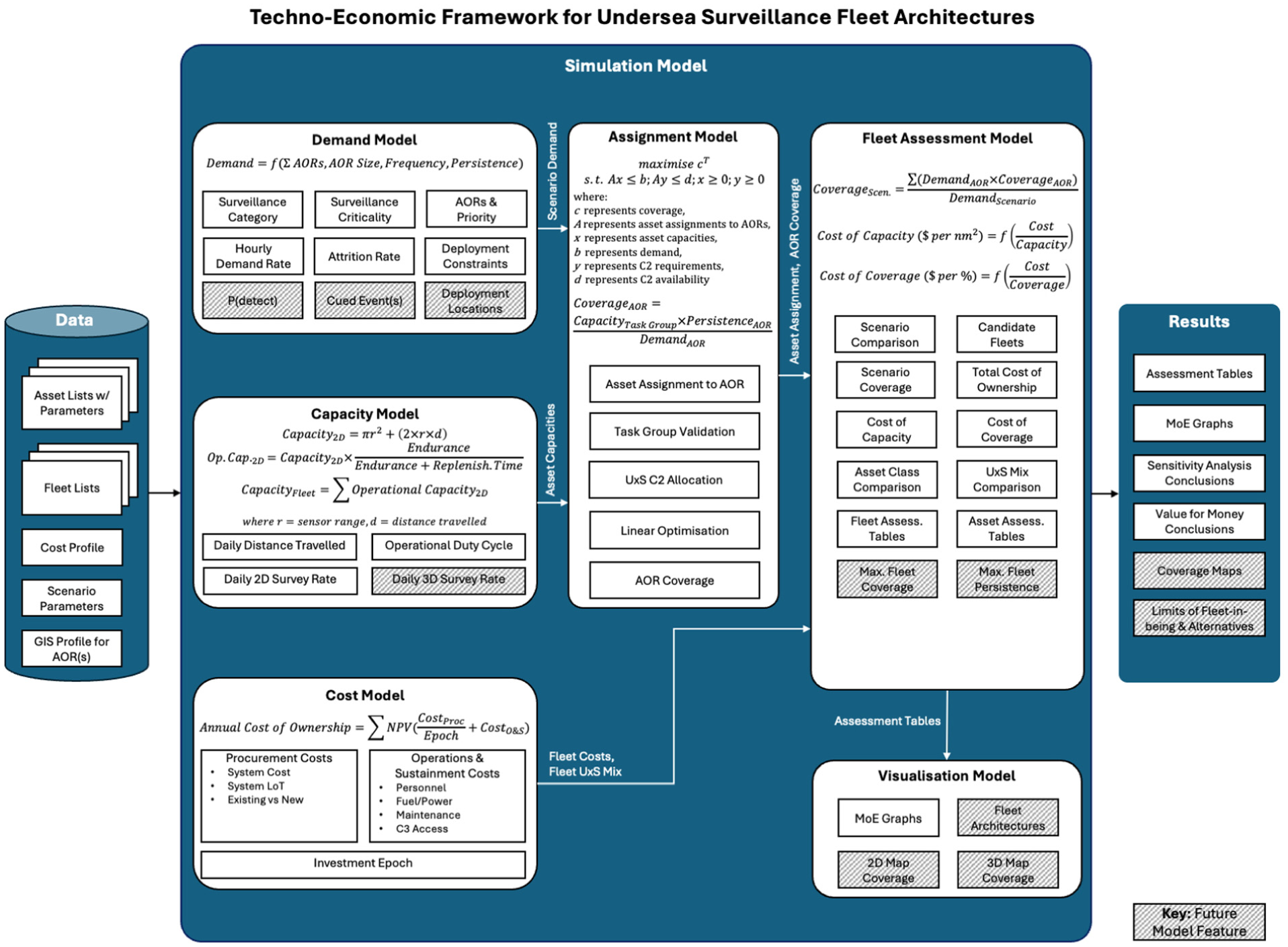
Proposed techno-economic framework for undersea surveillance.
3.1. Framework elements
The techno-economic framework shown in Figure 1 comprised three constituent elements: the input data, the simulation model, and the output results. The input data repository consisted of a collection of data files containing all the parameters required to execute the simulation model. This included:
Lists of naval assets, both crewed and uncrewed, relevant for conducting undersea surveillance. The asset lists included technical parameters for each asset, such as length, weight, transit speed, transit range, endurance, type of surveillance sensor, sensor range, and crew size. It also included procurement costs.
Lists of candidate fleets and the quantities of assets comprising each fleet.
Cost profile containing parameters to determine ongoing operations and sustainment costs for classes of assets.
Scenario parameters that define each surveillance scenario against which candidate fleets were assessed. This included the definition of each Area of Responsibility (AOR), the priority and criticality of each AOR, the persistence of surveillance required (duration that surveillance must be conducted), the level of conflict (e.g. wartime vs peacetime), and the associated availability of assets as well as the asset attrition rates during operations.
A Geospatial Information System (GIS) profile for each AOR where surveillance was conducted in the scenarios, including spatial extent and bathymetric characteristics.
The simulation model processed the input data, conducted the techno-economic assessment using the coded simulation, and generated the output results files. It contained sub-models for each contributing element of the analysis. The simulation model’s modularity allowed for the separation of concerns while integrating during execution for a holistic assessment. Further details on the modelling are provided in Section 4.
Finally, the output results were generated by the simulation model during execution. All results were generated concurrently and collated for each surveillance scenario and candidate fleet assessed. The results included both tabular exports of the raw assessment results and graphical representations of the results.
3.2. Framework characteristics
The techno-economic framework’s design had key characteristics that benefitted the research outlined in this article. These included a system of systems (SoS) approach, measures of effectiveness (MoE) based assessment, modularity, and computationally lightweight.
The framework utilised a system of systems approach to address considerations at the fleet architecture level. This facilitated a holistic assessment of alternate fleet architectures rather than drawing suboptimal conclusions based on isolated system or product suitability for undersea surveillance. The system of systems approach yielded insights at both the integrated fleet and individual asset levels. As Richmond 45 asserted about Systems Thinking approaches, ‘they can see both the forest and the trees; one eye on each’. Furthermore, taking an architectural top-down approach enabled the identification and prioritisation of parameters that most impact assessment outcomes. This facilitated the rapid narrowing of candidates in the trade space to feasible solutions. It also ensured that the research addressed the real-world problems and constraints of the application domain by quantifying value for money, a fundamental principle in acquiring Australian naval assets. 24
Following the SoS approach, the techno-economic framework based its assessment on MoE that were easy to interpret. MoEs centred the research on considerations that are directly linked to the application domain. MoEs such as Surveillance Capacity (nm2/day), Scenario Coverage (%), Annualised Total Cost of Ownership ($ p.a.) and Cost of Coverage ($ per %) were easy to understand and could be traced through the framework, such that the impact on results could be clearly identified at any part of the model.
Within the techno-economic framework, the sub-models were modular components, each focused on a distinct aspect of the analysis. The modular framework leveraged architectural patterns known to promote low coupling and high cohesion. 37 Low coupling reduced the interdependencies between sub-models, allowing them to be changed independently of each other. This also eased verification in model testing and validation of human-interpretable model inputs and outputs. With simple but clearly defined interfaces between the sub-models, high cohesion ensured the integrated simulation model yielded results consistent with each sub-model’s contributions. The modular framework was extensible, allowing additional sub-models to be incrementally added to build the model’s complexity or expand its scope to address additional research questions. The simulation model was intentionally decoupled from the input data, making it agnostic to the provided scenario, fleet, asset, and cost parameters. This made the simulation model readily reusable with new datasets.
A byproduct of the framework’s systems-of-systems approach and MoE focus was that its instantiation was computationally lightweight. Unlike physics-based models, this SoS-centric model had relatively simple calculations to analyse the MoEs. This meant the model did not rely on high-performance computing and could run quickly. The results shown in Section 5 were generated from simulation model execution that took less than ten seconds to run on a 2023 Apple MacBook Pro. The input data was able to be varied, and the model was then rerun many times in quick succession to yield larger sets of results for comparison.
4. Modelling method
This section describes the modelling method used by the research. It outlines the methods used within the simulation model and details of the constituent sub-models from the techno-economic framework shown in Figure 1. The simulation model was designed, coded and tested as a Python 46 software application. Each of the sub-models functioned as an individual software module within the application with defined software interfaces.
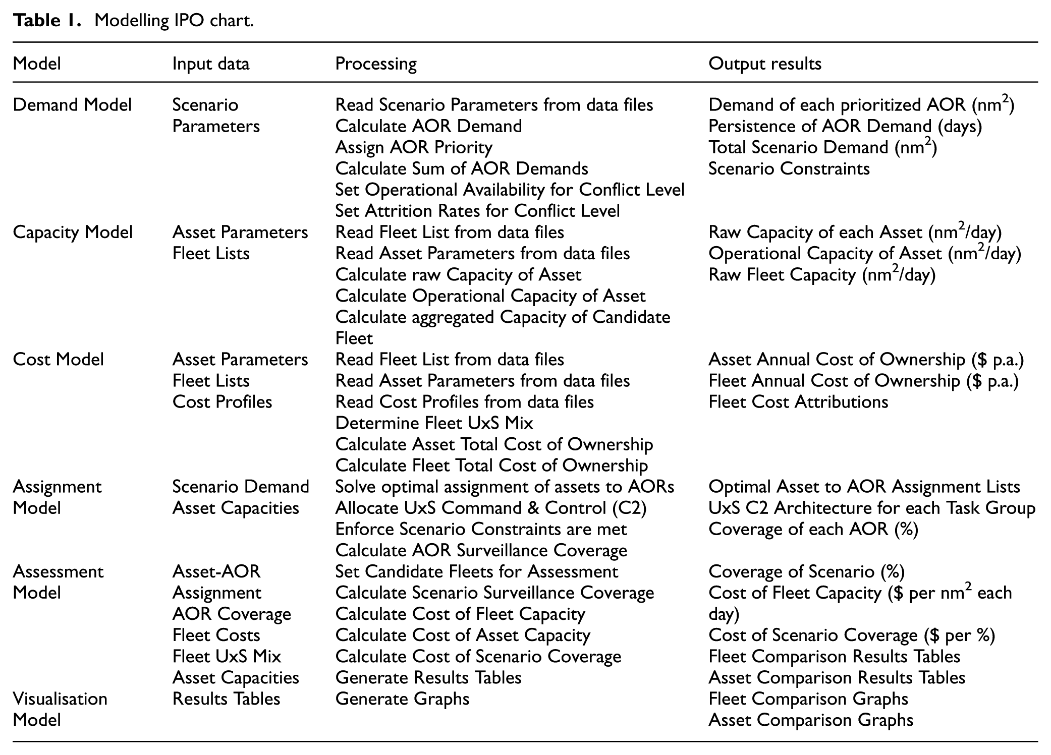
Table 1 below presents an Inputs-Processing-Outputs (IPO) chart summarising the role of each model within the techno-economic framework’s simulation. The following subsections provide a detailed description of each of these models, explaining the method of each model in terms of its construct and calculations, rather than the coding in Python.
Modelling IPO chart.
4.1. Demand model
The demand model ingested data relating to the surveillance scenarios and then constructed a representation of the surveillance demands placed on the candidate fleets. It encompassed all the requirements, constraints, and calculations necessary for simulating the scenario. The demand model did not include any modelling related to the candidate fleets or their surveillance assets. The outputs of the demand model, generally referred to as scenario demand, were provided to the assignment model.
The raw demand for each AOR within the scenario was calculated using Equation (1)
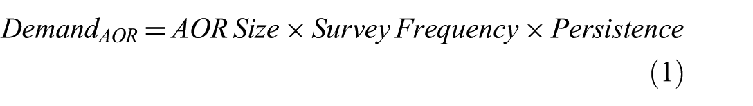
where AOR Size is the surveillance area in square nautical miles. Survey Frequency refers to the number of times per day that each point in the AOR must be surveyed, based on the AOR’s surveillance criticality. Since the entire AOR must be traversed before returning to survey the same point, this can also be expressed as how many times per day the AOR must be surveyed. Higher surveillance criticality results in a higher survey frequency. For example, a survey of critical undersea infrastructure may occur daily rather than monthly. Persistence is the duration of days for which the AOR must be surveyed.
The total demand of the surveillance scenario was calculated using Equation (2)

where n is the number of AORs in the surveillance scenario.
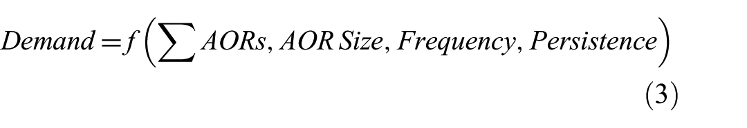
Thus, surveillance demand was expressed as the following abstract function in Equation (3), also shown in the framework in Figure 1
In addition to the quantitative scenario demand measurements, the demand model also defined scenario constraints that impacted the ability of candidate fleets to survey the individual AORs and the overall scenario. This included factors such as the relative priority of AORs within the surveillance scenario. The demand model also established the fleet operational availability profile (the percentage of surveillance assets ready for deployment) and the asset attrition rate profile (the percentage of assets lost during surveillance) based on the scenario’s conflict level (peacetime vs wartime). Both of these profiles were scenario-dependent and included a range of availability and attrition values for different classes of surveillance assets.
4.2. Capacity model
The capacity model calculated the surveillance capacity of each asset within a candidate fleet. This model was independent of the simulated surveillance scenario constructed by the demand model. The output of the capacity model was the collection of asset capacities for a candidate fleet, which was provided to the assignment model.
The capacity model read the data files containing asset parameters and fleet lists. For each asset in each candidate fleet list, the model first calculated its raw two-dimensional surveillance capacity. The raw capacity was then converted to the asset’s operational capacity, based on its operational duty cycle, which represents the percentage of time it remains on station conducting surveillance. This operational capacity provided a more accurate representation of an asset’s persistent surveillance capacity over an extended duration in the scenarios. Each asset’s two-dimensional surveillance capacity was measured as the area of ocean surveyed per day. An aggregated capacity for each candidate fleet was then calculated as the sum of the capacities of the assets within that fleet.
The asset’s daily capacity, when viewed from above, is shown in Figure 2. This approximates the maximum daily capacity based on straight-line movement of the asset and was calculated using Equation (4)

where r is the asset’s sensor range. d is the distance the asset travels in a day.
Daily surveillance capacity of a single asset.
Note that the daily capacity shown in Figure 2 is based on a 360° field of view for the combination of sensors on the asset. This is an approximation and will not be the case for all assets and sensors.
The asset’s operational daily capacity was then calculated as
where Endurance is the duration an asset can remain operationally deployed. Replenishment Time is the duration required to prepare an asset for redeployment. This may include refuelling, a crew refresh, restocking supplies, and any necessary technical or safety checks. It does not include the transit time to return to the replenishment location or deep maintenance. Replenishment Time is during the asset’s operational deployment when not on station conducting surveillance.
The aggregated fleet capacity was calculated as
where n is the number of assets in the candidate fleet.
4.3. Cost model
The cost model calculated the total cost of ownership of each surveillance asset within a candidate fleet. This cost included both procurement costs (capital expenditure) as well as operations and sustainment costs (operations expenditure). The cost model was independent of the simulated surveillance scenario constructed by the demand model and the capacity calculations in the capacity model. In addition to cost calculations, the cost model also characterised a candidate fleet list’s mix of uncrewed systems by investment magnitude and by the categories of uncrewed assets (small tactical, large strategic, or hybrid mix of both). The output fleet costs and fleet mix were provided to the assessment model.
Like the capacity model, the cost model also read the data files containing asset parameters and fleet lists, but extracted the unit cost data rather than performance data. In addition, the cost model imported the applicable cost profile from the data files that contained operations and sustainment costs for different types of surveillance assets. Using this data, the cost model calculated the annual cost of ownership of a candidate fleet. The cost model determined which assets in the candidate fleet were new and extracted their procurement cost from the data files. Procurement costs were then amortised over the defined investment epoch (repayment period) to determine their contribution to annual fleet costs. The cost model extracted ongoing operations and sustainment costs from the defined cost profile as an aggregated hourly rate for different types of surveillance assets. This hourly rate was then extrapolated to a yearly cost to determine each asset’s contribution to the annual fleet costs. The annual procurement costs and annual operations and sustainment costs were summed to determine the annual total cost of ownership of a candidate fleet. The cost model also handled converting past or future costs to current cost figures using the net present value (NPV) method.
Thus, the annual fleet cost was expressed as the following abstract function, as shown in the framework in Figure 1
where n is the number of assets in the candidate fleet, NPV is the net present value,
Note that the asset procurement cost (
4.4. Assignment model
The assignment model used the scenario demand and the candidate fleet’s asset capacities to assign each surveillance asset to an AOR in the scenario and then determined the surveillance coverage of each AOR. First, the assignment model determined the optimal assignment of each asset in the candidate fleet to an AOR in the surveillance scenario. The selected assets for each AOR were analogous to the assignment of a naval task group to conduct a mission. The assignment of assets to AORs served three key purposes as part of the systems-of-systems approach to modelling:
It determined the realistic maximum surveillance coverage that a candidate fleet could achieve by not splitting single asset capacity between multiple AORs, and ensuring assets were not wasted through the assignment of capacity that exceeds the demand of an AOR. This asset-level granularity could not be captured by comparing total fleet capacity with total scenario demand.
It ensured that all the scenario constraints were met when calculating a candidate fleet’s surveillance coverage. For example, guaranteeing each AOR was surveyed with the persistence and frequency required by its criticality, and that the set of AORs was serviced in order of priority.
It formed valid task groups that were allocated to each AOR, with sufficient Command & Control (C2) architectures in place for managing the assigned uncrewed systems.
Linear programming, a mathematical technique within Operations Research, was used to solve this general assignment problem. The assignment model optimised the assignment of assets to each scenario AOR in descending priority order by sequentially allocating the fleet assets that met the demands of the AOR, and met all scenario constraint rules, while minimising the allocated capacity (to prevent over-allocation and wasted assets).
A weighted C2 points system was used as an additional constraint rule to ensure sufficient C2 architectures were available for the uncrewed systems in the task group allocated to the AOR. For each type of asset, C2 points were assigned to crewed systems based on their C2 capabilities, and C2 point requirements were established for uncrewed systems according to their C2 demands and level of autonomy. The points system ensured that only valid task groups were formed for each AOR where the C2 budget met or exceeded the C2 costs of the collective surveillance assets.
A candidate fleet (representing all assets owned by the Navy) is never 100% available for operations, so the assignment model allocated a subset of the total fleet assets to the scenario AORs. For a given candidate fleet, the assignment model reduced the quantity of assets assigned to the AORs based on the scenario’s operational availability and attrition rates for each asset type. For example, a wartime scenario had a larger quantity of assets from the candidate fleet that were operationally available compared to a peacetime scenario, but the attrition rate was higher. Depending on constraints from the demand model, individual AORs had further restrictions on the quantity of assets that could be assigned from the overall fleet.
When applied across the set of AORs in the scenario, this linear programming maximised the surveillance coverage subject to not over-allocating capacity to AOR demands and not exceeding asset constraints within the scenario (including C2 availability). This was expressed as the following general linear programming equation from the framework shown in Figure 1
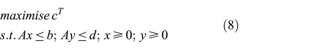
where c represents surveillance coverage, approximated as the sum of each AOR coverage calculated by Equation (9),
With the linear programming’s assignment of surveillance assets to scenario AORs in task groups, the assignment model calculated the coverage of each AOR as follows
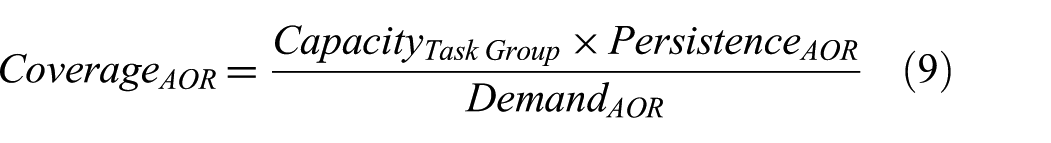
where
4.5. Assessment model
The assessment model conducted the overall techno-economic assessment of numerous candidate fleets in alternate surveillance scenarios based on multiple executions of the demand model (varying surveillance scenario), capacity model (varying capacity of fleets with different assets), cost model (varying cost of fleets with different assets), and assignment model (varying coverage achieved by different fleets across different scenarios). The techno-economic assessment of candidate fleets was achieved by integrating the technical feasibility of scenario coverage with the financial viability of total cost of ownership. This was measured for each candidate fleet as the Cost of Coverage. The assessment model also evaluated individual assets to compare their contributions, utility, and value for money in the surveillance scenarios simulated by the model. Results tables from the techno-economic assessment were generated by the assessment model and written to files for post-simulation analysis. The results tables were also provided to the visualisation model to create graphs.
The assessment model began by determining the candidate fleets to be assessed and the surveillance scenarios that would serve as the basis for each assessment. For each scenario, the demand model was executed, followed by the execution of the capacity, cost, and assignment models for each candidate fleet.
For each candidate fleet in each scenario, the assignment model provided the allocation of fleet surveillance assets to each AOR within the scenario. Then, with the coverage of each AOR provided by the assignment model, the assessment model calculated the aggregated surveillance coverage of the entire surveillance scenario as follows:
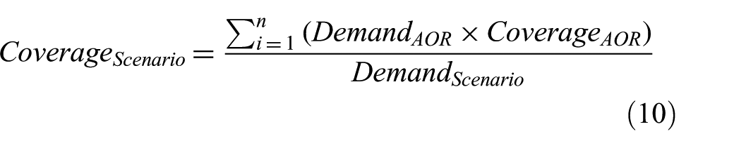
where n is the number of AORs in the surveillance scenario.
The scenario coverage was the overall technical evaluation of each candidate fleet against a specific surveillance scenario. As a percentage figure, the scenario coverage served as a MoE for easy comparison between the fleets. To then integrate economic evaluation, the total cost of ownership for each fleet was obtained from the cost model. Integrating the data from the models yielded two techno-economic MoEs to assess the value for money of each candidate fleet: the cost of capacity and the cost of coverage. Cost of capacity was an intermediate techno-economic measure based on raw fleet capacity and total cost of ownership. It was independent of any surveillance scenario and therefore didn’t assess the candidate fleet’s ability to meet the constraints of the scenario or the complexities in forming valid task groups for assignment to AORs. Cost of coverage was a more comprehensive techno-economic measure as it accounted for the candidate fleet’s ability to meet the needs of a surveillance scenario and the total cost of ownership. The cost of coverage for each candidate fleet varied when changing the scenario parameters, but the cost of capacity remained unaffected. The generalised expressions for the cost of capacity and the cost of coverage are outlined below, as shown in the framework in Figure 1. Both of these techno-economic MoEs facilitated easy comparison of the value for money of candidate fleets

where

where
Finally, the assessment model collated all the results from the simulation and saved the tabular results to comma-separated values (CSV) files. To assist in the interpretation of the results with respect to the research questions in Section 2, the results tables included the categorisation of fleets by their mix of uncrewed systems: investment/budget percentage expended on uncrewed systems as a portion of the overall fleet, and the focus on small tactical uncrewed systems or large strategic uncrewed systems or a hybrid mix of both. Similarly, the results tables comparing individual assets were categorised by asset classes for ease of comparison.
4.6. Visualisation model
The visualisation model used the fleet assessment data, including results tables from the assessment model, to generate graphs as visual representations of the results. Its purpose was to create graphs that made it easier to interpret the MoE trends in the results compared to reading tables alone. Producing the graphs as part of the simulation rather than during post-simulation analysis ensured consistency between multiple simulation runs and reduced the chances of inadvertent errors when translating from tables to graphs. All the graphs generated by the visualisation model were saved as portable network graphics (PNG) files.
Unlike the other models, the visualisation model did not perform any calculations. This decoupled it from the assessment and reduced the chances of errors when generating the results charts.
5. Results
This section of the article summarises the research results from conducting multiple executions of the simulation model described in Section 4.
5.1. Data used for modelling
As outlined in Section 4, the simulation model was decoupled from the data being analysed by the model during each execution. This allowed the research modelling to be conducted with open-source data without impacting the simulation model itself. The results in this section were generated using unclassified and open-source data for asset performance, fleet composition, cost profiles, and surveillance scenarios. The asset data and fleet data used to create these results are summarised in Appendix A and Appendix B, respectively. This open-source data is valid for drawing conclusions on the utility of different uncrewed assets in performing undersea surveillance for the scenarios modelled. The use of open-source data is consistent with other published studies conducting modelling and simulation of military applications.11,30 The results could be further extended to include specific findings for the Navy by re-running the simulation model using classified performance data and scenario parameters.
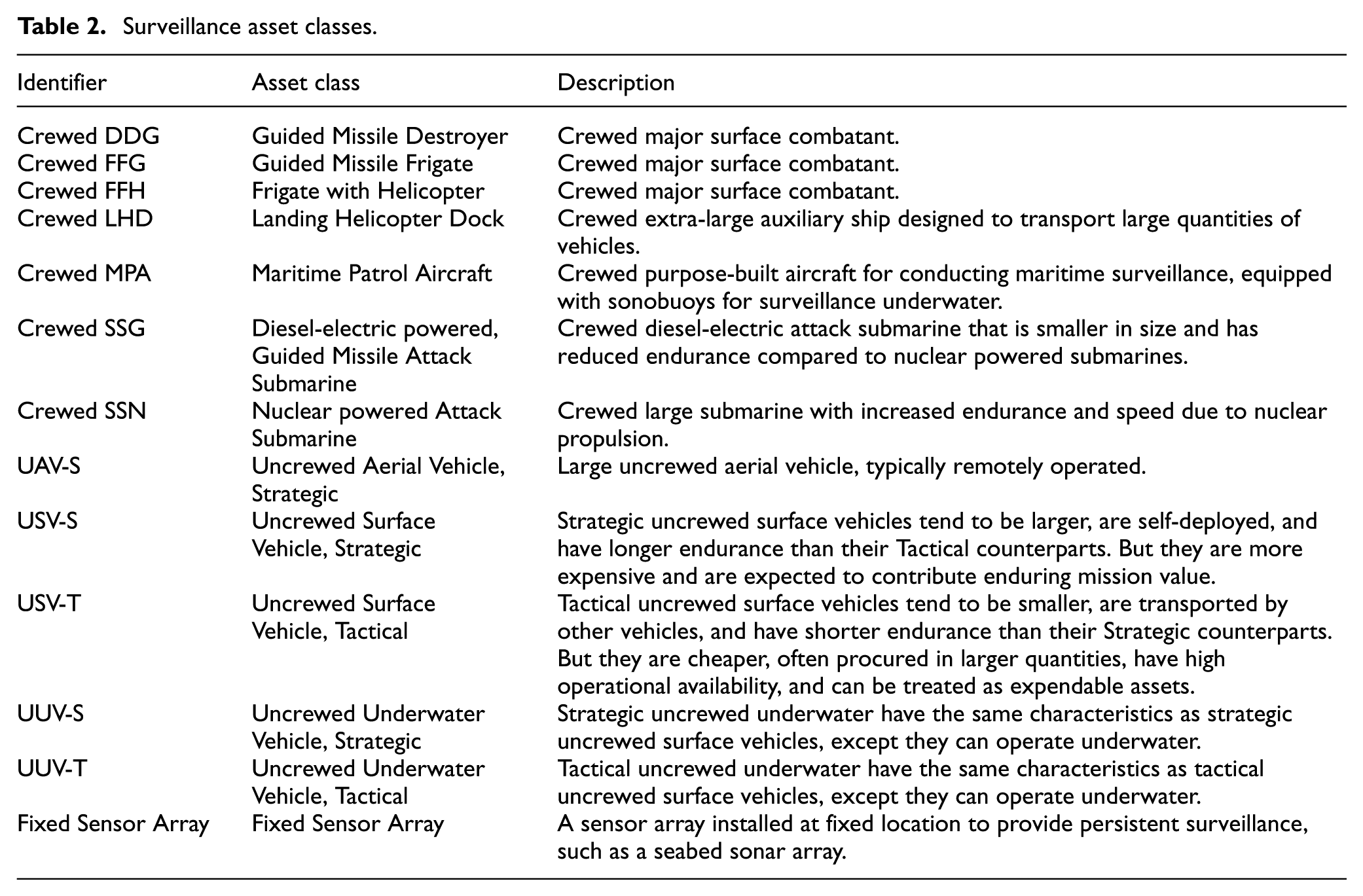
To ease the interpretation of trends in the results, the surveillance asset data identifies the classes of assets used to categorise the various systems. The effectiveness of different classes of assets in performing undersea surveillance is more important than the performance of specific products for addressing the research questions. The asset classes used are listed in Table 2.
Surveillance asset classes.
Forty candidate fleet architectures were designed for this research and assessed by the techno-economic model. Each candidate represented the RAN’s fleet for maritime surveillance at a forecast year, starting with the current year of modelling (2025) and projecting forward in 5-year increments up to 2040. Candidate fleets were differentiated based on their investment in uncrewed systems, varying from 0% to 20% of the fleet’s total cost of ownership. This was designed to compare the techno-economic assessments of alternative fleets with varying levels of uncrewed system adoption, including the continuation of a completely crewed fleet. For fleets incorporating uncrewed systems, candidate fleets varied their investment in the adoption of strategic, tactical, or a hybrid mix of both strategic and tactical uncrewed systems, in order to assess the utility of different types of uncrewed systems.
Four example surveillance scenarios were constructed for the simulation model runs. These surveillance scenarios were based on the United States Navy missions described by Button et al. 28 and Savitz et al. 26 but adapted to AORs in the Australian maritime environment. The scenarios included surveillance demands representing missions such as persistent intelligence, surveillance, and reconnaissance (ISR), mine countermeasures (MCM), anti-submarine warfare (ASW), and undersea cable monitoring. The four scenarios varied between a baseline level of demand and high demand (26.4 vs 106.5 million square nautical miles over 90 days), as well as between peacetime and wartime conditions. The results of the techno-economic modelling of each candidate fleet against each of these scenarios are shown in the rest of this section.
5.2. Fleet capacity results
Figure 3 is a results graph generated by the simulation model, showing the surveillance capacity of the candidate fleets assessed. The colour of each series identifies the uncrewed systems investment for each fleet, and the datapoint shape determines the type of uncrewed systems the investment was focused on. As time progresses along the x-axis, the graph illustrates the ongoing impact on surveillance capacity of investing in uncrewed systems. As outlined in Section 4, capacity is modelled independently of demand, so the same fleet capacity results were obtained across each of the surveillance scenarios. The graph shows that higher investment in uncrewed systems yields greater fleet surveillance capacity, particularly when investing in strategic or a hybrid mix of uncrewed systems. The positive delta in surveillance capacity for fleets with uncrewed systems increases over time as the investment continues to be made.
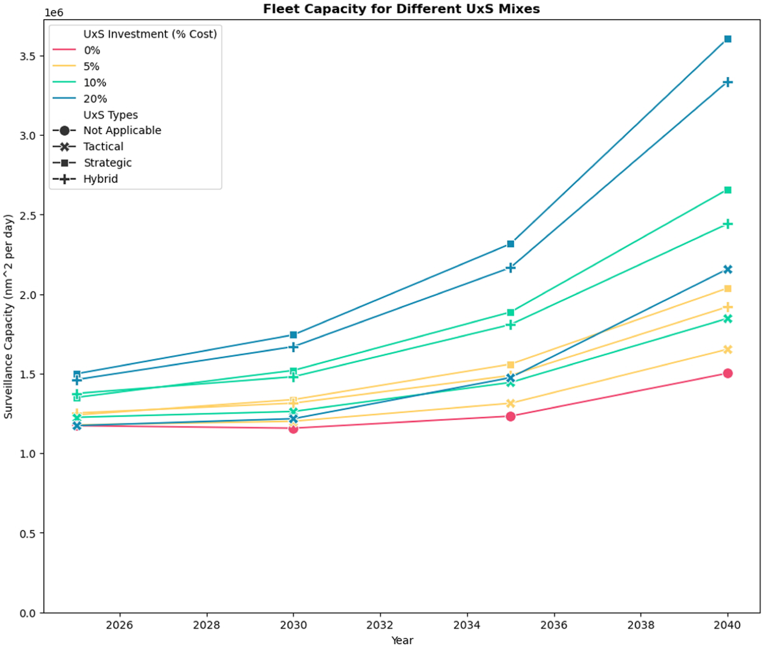
Fleet capacity results graph.
5.3. Scenario coverage results
Figure 4 is another results graph generated by the simulation model, showing the scenario coverage of the candidate fleets assessed for each of the four surveillance scenarios. The colour of each series identifies the uncrewed systems investment for each fleet, and the datapoint shape determines the type of uncrewed systems the investment was focused on. As time progresses along the x-axis, the graphs illustrate the ongoing impact on scenario coverage of investing in uncrewed systems under different surveillance circumstances. As outlined in Section 4, scenario coverage is based on modelling the scenario demand, fleet capacity, and task group assignment. The scenario coverage results are presented across four graphs, one for each scenario. Similar to surveillance capacity, these graphs indicate that higher investment in uncrewed systems yields greater surveillance coverage, particularly when investing in strategic or a hybrid mix of uncrewed systems. However, compared to raw capacity in the previous graph, the advantage of strategic uncrewed systems over tactical uncrewed systems is even greater for surveillance coverage that must meet all the scenario and task group assignment constraints. The benefit of uncrewed systems is slightly higher in peacetime than in wartime. Higher demand scenarios take greater advantage of larger investments in uncrewed systems because the results do not reach the limit of 100% scenario coverage.
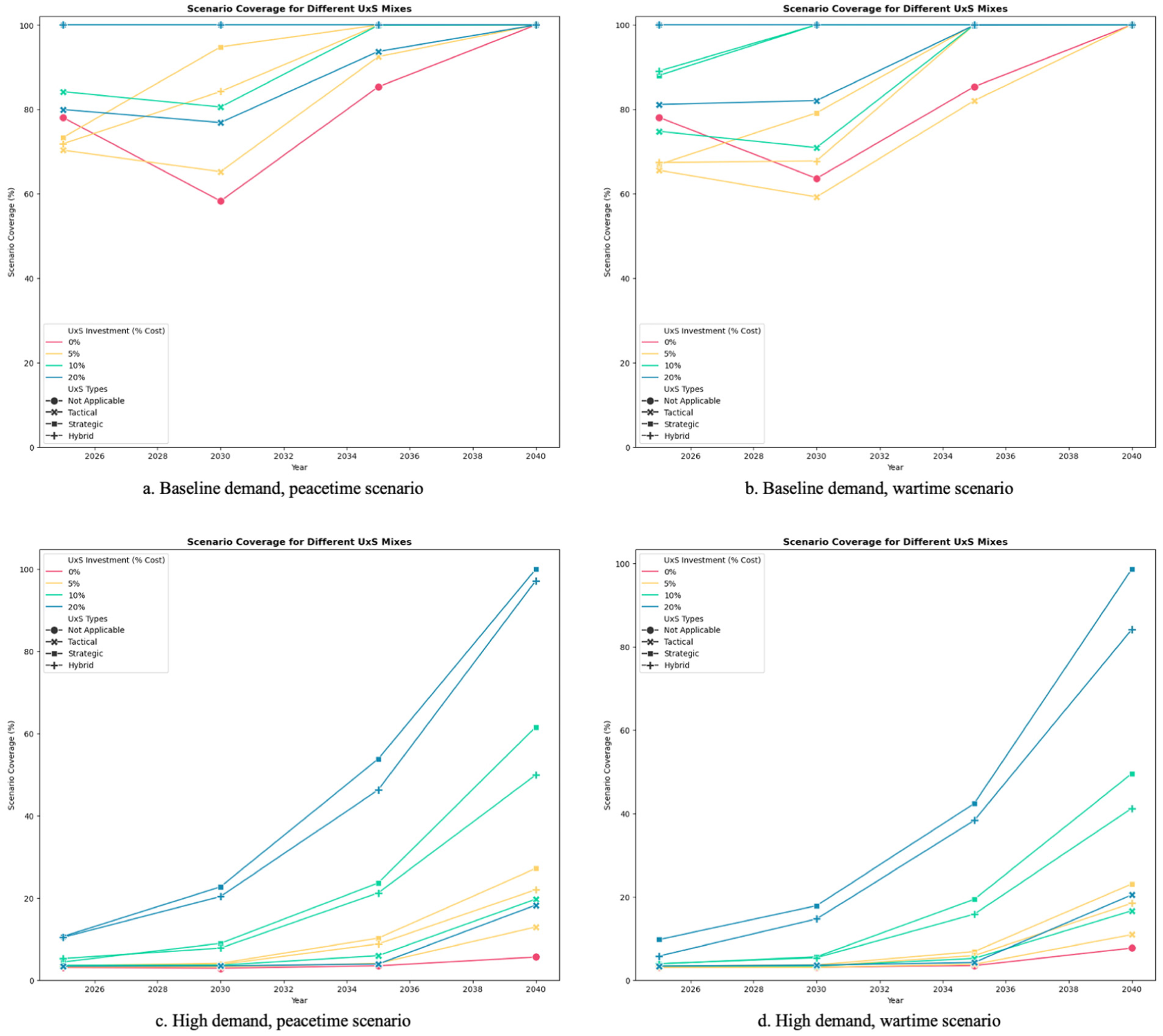
Scenario coverage results graphs (the crewed fleet’s dip in coverage of baseline demand in 2030 is due to the timing of crewed assets being decommissioned ahead of new assets being commissioned in the following years).
5.4. Total cost of ownership results
Figure 5 is another results graph generated by the simulation model, showing the total cost of ownership of the candidate fleets assessed. The stacked colour of each column identifies the attribution of costs towards procurement and operations & sustainment for both crewed and uncrewed systems in each fleet. As outlined in Section 4, the cost is modelled independently of demand, resulting in the same fleet capacity results across all surveillance scenarios. In most cases, annual operations & sustainment costs outweigh annual procurement costs.
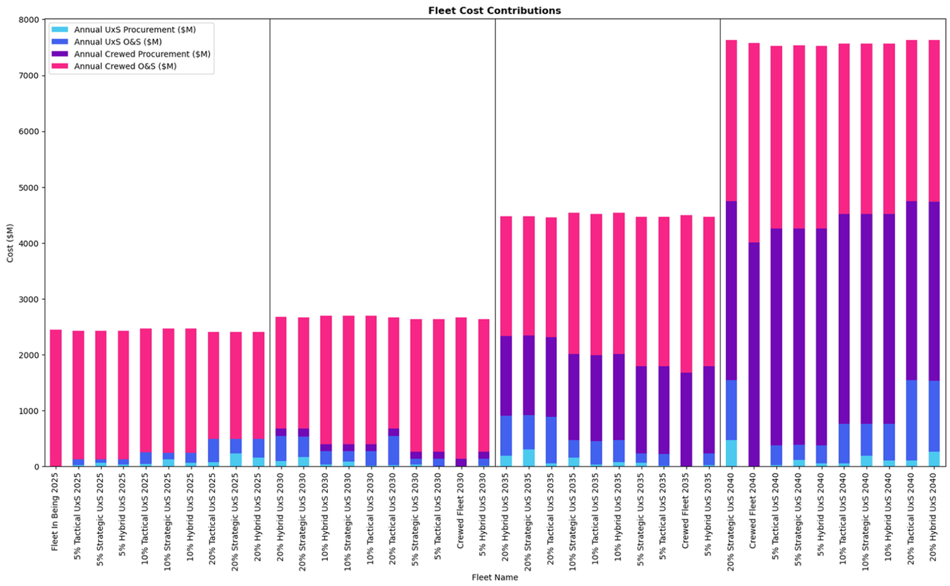
Total cost of ownership results graph.
5.5. Techno-economic assessment results
The following two figures illustrate the results of the techno-economic assessment of the candidate fleets, integrating the prior technical and economic evaluation results. They are based on the techno-economic MoE outlined in Section 4.
Figure 6 is a results graph generated by the simulation model, showing the cost of capacity of the candidate fleets assessed. The colour of the columns identifies the uncrewed systems investment for each fleet. The candidate fleets are chronologically sorted from 2025 to 2040, then by ascending cost of capacity. Cost and capacity were assessed independently of demand, so these techno-economic results were the same regardless of the surveillance scenario modelled. For each modelled year, candidate fleets with higher investment in strategic or a hybrid mix of uncrewed systems have the lowest cost of capacity.
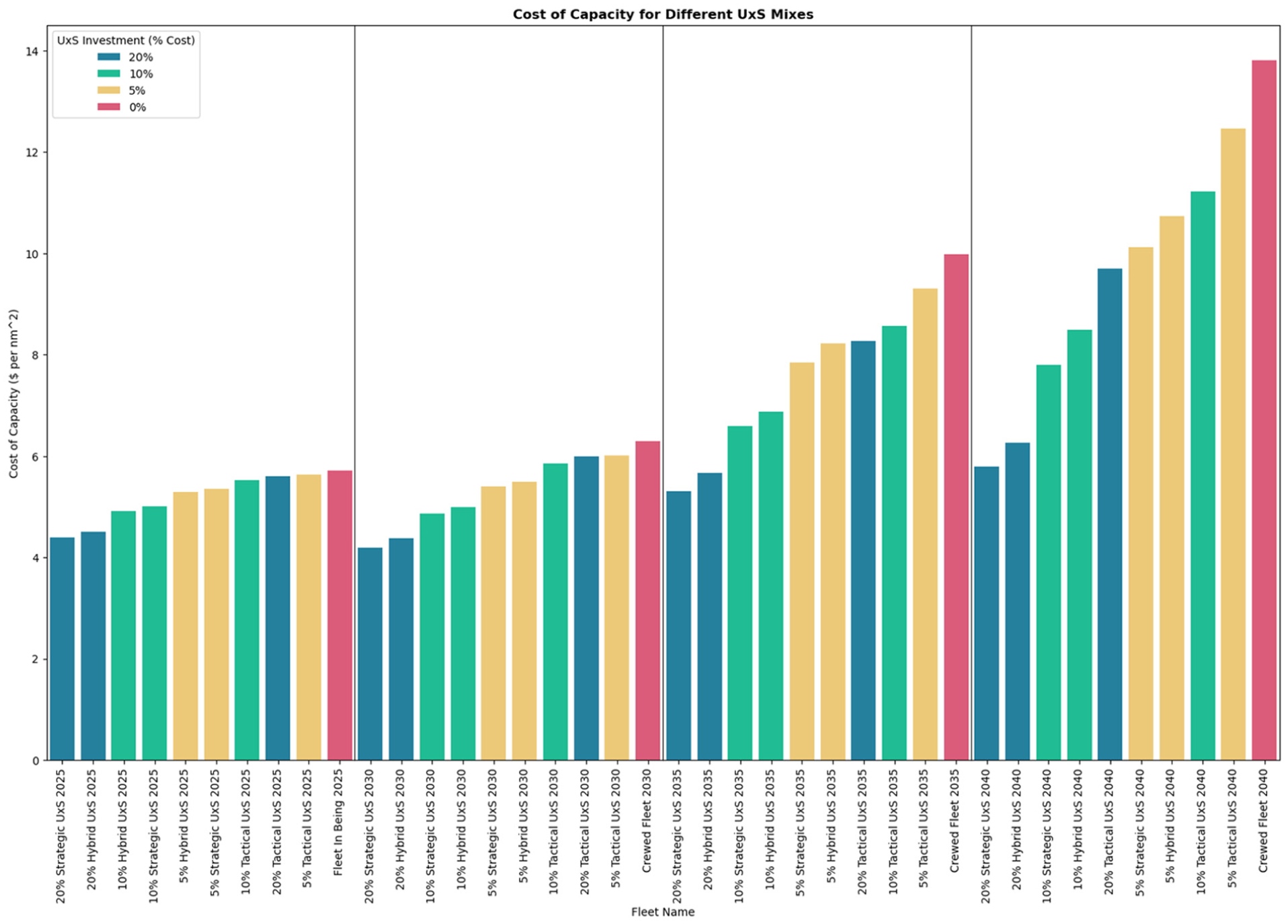
Cost of capacity results graph.
Figure 7 shows further results graphs generated by the simulation model, which display the cost of coverage for the candidate fleets assessed. These are the most comprehensive results graphs generated by the model. They illustrate value for money, taking into consideration the scenario demands, fleet capacity, task group assignment, the scenario coverage, and the fleet total cost of ownership. The colour of the columns identifies the uncrewed systems investment for each fleet. The candidate fleets are chronologically sorted from 2025 to 2040, and then by ascending cost of coverage. For each modelled year, candidate fleets with higher investment in strategic or a hybrid mix of uncrewed systems have the lowest cost of coverage. Comparing the graphs highlights that the utility of strategic over tactical uncrewed systems for surveillance coverage is greater in wartime than peacetime.
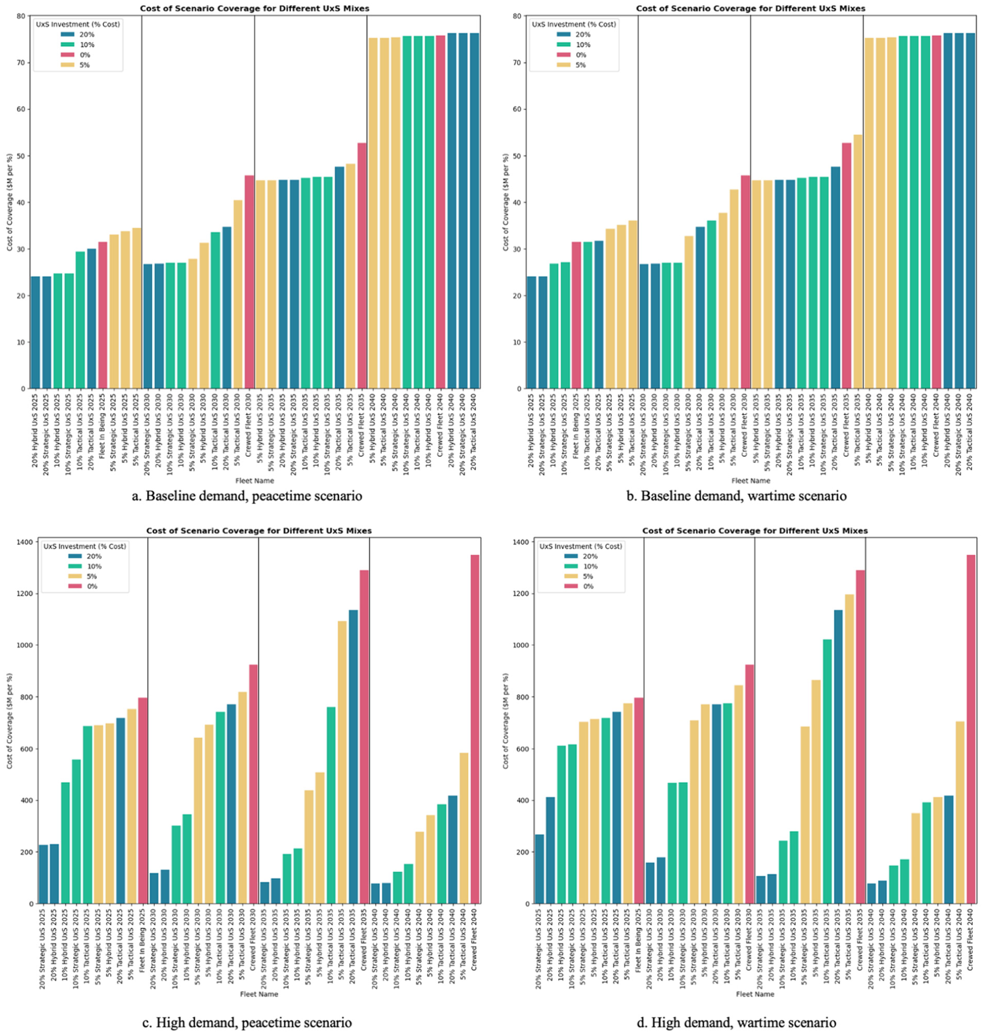
Cost of coverage results graphs.
Figure 8 is an additional techno-economic results graph generated by the simulation model. However, instead of comparing candidate fleets, it compares classes of surveillance assets. It illustrates the techno-economic assessment of assets by comparing the asset surveillance capacity with the cost of operations and sustainment. Note that the cost metric used in this graph excludes procurement costs to provide a steady-state comparison of assets after the investment epoch has concluded and procurement costs have been paid. The graph shows the daily surveillance capacity for different asset classes, per million dollars of operations and sustainment costs from the annual budget. In this graph, strategic uncrewed surface vehicles have the largest surveillance capacity per dollar.
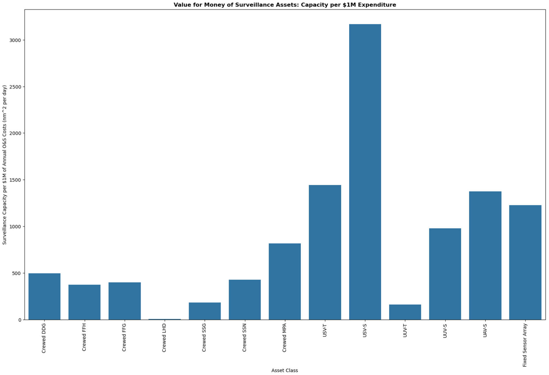
Asset capacity per annual costs graph.
6. Discussion
This section discusses the implications of the results in Section 5, how they address the research questions defined in Section 2, and future directions for further research. Generally, the results indicate that larger investments in uncrewed systems provide greater surveillance coverage, with strategic uncrewed systems contributing the greatest value for money. The utility of these uncrewed systems was demonstrated over a range of surveillance conditions. Furthermore, the results have demonstrated the ability of the techno-economic framework and model to support holistic decision-making on RAN fleet design. However, the model could be further enhanced with GIS modelling, which is recommended for future research. These insights are discussed and elaborated further below.
6.1. Answers to research questions
Based on the research results presented in the previous section, responses to each of the research questions are provided below, accompanied by evidence-based conclusions.
As shown in the graphs in Figure 4, the absolute value of surveillance coverage for the candidate fleets varies depending on the level of demand. In the baseline demand scenarios, the candidate fleets achieved between 60-100% coverage, which increased over time. For the high-demand scenarios, most of the candidate fleets achieved less than 25% coverage, with only the 20% investment in a strategic or hybrid mix of uncrewed systems approaching 100% coverage in the final year modelled. In the high-demand wartime scenario (Figure 4, graph d), the results show that over the forecast period from 2025 to 2040, the projected crewed fleet achieves approximately 6% scenario coverage. Alternatively, by redirecting 5%, 10%, or 20% of the annual fleet budget towards strategic uncrewed systems, scenario coverage increases to approximately 22%, 51%, or 100% respectively.
There are clear trends in the scenario coverage results that yield more valuable insights into the relative coverage achieved by the candidate fleets. Except for the first year, when uncrewed systems were initially being procured, the candidate fleets incorporating uncrewed systems provided greater surveillance coverage than the crewed fleet (the only exception is candidate fleets with 5% investment in tactical uncrewed systems because the investment yields only a small amount of surveillance capacity from the tactical uncrewed assets, while requiring the divestment of a small quantity of high capacity crewed assets). Candidate fleets with higher investment in uncrewed systems achieved higher surveillance coverage, evidenced by the blue, green, and yellow series in Figure 4. This is consistent with existing research,2,47–50 which established the ability of uncrewed systems to provide greater surveillance capacity for the same expenditure. Note that this trend does not extend to 100% investment in uncrewed systems. Depending on the fleet’s mix of uncrewed systems, a threshold is reached where further investment in uncrewed systems results in decreased surveillance coverage. This is because the divestment of crewed assets results in insufficient C2 architectures to deploy the uncrewed systems. The modelling thereby provides evidence that C2 is a key enabler for the employment of uncrewed systems, as previously asserted by Clark and Patt, 51 Savitz et al. 26 and Gargalakos. 52
Furthermore, investment in strategic uncrewed systems yielded greater surveillance coverage than tactical uncrewed systems. Investment in a hybrid mix of uncrewed systems resulted in coverage that was close to, but not as high as, that of strategic uncrewed fleets. This is highlighted in Figure 4 by comparing the series with different datapoint shapes for the same level of investment (same colour). The tactical uncrewed fleets had substantially lower coverage and were exceeded by strategic uncrewed fleets with a lower investment percentage (for example, see Figure 4 graph c., where the 10% Tactical series has lower surveillance coverage than the 5% Strategic and 5% Hybrid series). These results provide evidence that supports the Royal Australian Navy’s pursuit of strategic uncrewed systems such as the Anduril Ghost Shark and C2 Robotics Speartooth, and the United States Navy’s investment in Sea Hunter and Orca uncrewed systems.22,51
However, the relative surveillance coverage of tactical vs strategic uncrewed fleets may vary when incorporating GIS modelling into the simulation. The transit time of self-deployed strategic assets compared to transported tactical assets is expected to have a noticeable effect on the surveillance coverage, as is the replenishment time and reliance on crewed assets within the assigned task groups. This is discussed further in the subsections on limitations and future research.
When considering the coverage results in light of the modelling method, it was noted that the assignment model’s linear programming solver optimises asset assignment to survey the AORs in scenarios’ order of priority, while minimising any waste from excess capacity or C2 points assigned to an AOR’s task group. It doesn’t treat all the AORs as equal priority when assigning surveillance assets. Therefore, the highest coverage results were achieved in this modelling by:
Spreading the crewed assets across all of the scenario’s AORs to prevent wasted surveillance capacity and distribute C2 points for employment of uncrewed systems.
Allocating the highest capacity uncrewed systems (generally, strategic uncrewed vehicles) to AORs in priority order without exceeding the AOR demand.
Allocating the lower-capacity uncrewed systems (generally, tactical uncrewed vehicles) to AORs last to fill any capacity gaps in priority AORs, or en masse to low-priority AORs if there are no remaining high-capacity assets for these final AORs.
This is similar to the observations from Laan et al. 53 and Craparo and Karatas 19 that used linear programming to determine the optimal placement of maritime assets for ASW scenarios. However, the coverage results in this article extend beyond a single operation to optimise the fleet’s coverage of multiple concurrent AORs and mission types.
The scenario coverage results showed that the impact of uncrewed systems was greater in higher-demand scenarios (Figure 4, graphs c. and d.). In the baseline demand scenario (Figure 4, graphs a. and b.), the utility of uncrewed systems was not fully realised as the crewed fleets still achieved high surveillance coverage when the demand was low. Therefore, the incorporation of uncrewed systems is best suited to surveillance conditions where the overall demand is high, particularly if it exceeds the crewed fleet’s raw capacity of approximately 1.2-1.5 million square nautical miles per day (shown by the red 0% series in Figure 3). The utilisation of uncrewed systems for undersea surveillance may still be valued below this threshold, as it allows multi-role crewed assets to be reassigned to other naval tasks as shown by Martin et al. 25 but is beyond the scope of this study.
The utility of uncrewed systems in peacetime vs wartime surveillance conditions had only minor variations (comparing Figure 4 graphs a. and c. with graphs b. and d.). The delta between the crewed fleet coverage and uncrewed fleet coverage was slightly higher for peacetime scenarios. The advantage of strategic over tactical uncrewed systems decreased slightly for wartime scenarios due to the changes in asset operational availability and attrition rates. The results provide new evidence of the advantages of uncrewed systems and their suitability for both conditions. While other studies47,54,55 have analysed uncrewed systems in operational scenarios of varying conflict levels, they have not explicitly compared and drawn such conclusions.
Conclusions on the best geographical areas for adopting uncrewed systems cannot be drawn from the results in this article. The simulation model must include GIS modelling to conduct an analysis of uncrewed systems in different geographical areas. This is discussed further in the subsections on limitations and further research.
Based on the asset capacity and cost results, the strategic uncrewed surface vehicles (e.g. Sea Hunter) provided the highest surveillance capacity per dollar spent on enduring operations and sustainment costs. This is shown in Figure 8. These results are consistent with other studies that have asserted the benefits of incorporating USVs into naval fleets. 10 For crewed systems, the maritime patrol aircraft (e.g. P-8 Poseidon) provided the highest capacity per dollar, although it is still not as high as that of the strategic uncrewed surface vehicles. This is also shown in Figure 8. Note that this is a measure of asset capacity only and does not account for all the scenario demand needs, such as surveillance persistence.
Analysing the coverage results more broadly, it was concluded that strategic uncrewed systems provide the most significant improvement to the holistic undersea surveillance needs, as evidenced by the respective candidate fleets providing the highest scenario coverage in Figure 4. Fleets incorporating strategic uncrewed systems also had the lowest cost of coverage for each year, as shown in Figure 7, representing the largest improvement per dollar spent. This is further evidence supporting the RAN’s adoption of strategic uncrewed maritime systems in AUKUS Pillar II. 51
Conclusions on value for money are best drawn from the cost of coverage results. For a consistent comparison between candidate fleets, the results were interpreted on a year-by-year basis as all fleet costs increased over time. For any given year, a 20% investment in strategic or hybrid uncrewed systems yielded the lowest cost of coverage, as shown in Figure 7 (the only exception is in low-demand scenarios where many fleets achieved 100% coverage and therefore the cost of coverage remained similar between candidate fleets, as excess capacity had no impact on coverage beyond 100%).
As noted above, value in this study was considered purely from the perspective of surveillance coverage. It did not account for other constraints, roles, or needs for the naval assets within each candidate fleet. Therefore, the following return on investment conclusions are noted for consideration in a broader context of naval fleet architectures and budget appropriation:
For the lower-demand peacetime scenario in Figure 4 graph a., a return on investment was realised immediately for all 10% and 20% investments in uncrewed systems, as these fleets achieved higher coverage than the crewed fleet in 2025. A 5% investment in uncrewed systems yielded a return in 2030 for strategic and hybrid uncrewed systems, and by 2035 for tactical uncrewed systems.
For the lower-demand wartime scenario in Figure 4 graph b., a return on investment was realised immediately for 10% strategic and hybrid fleets, as well as all 20% investments in uncrewed systems. The remaining uncrewed fleets realised a return on investment by 2030, but the 5% tactical uncrewed system fleet did not realise a return for this scenario.
For both higher-demand scenarios in Figure 4 graphs c. and d., all candidate fleets investing in uncrewed systems realised an immediate return on investment in 2025 with higher surveillance coverage than the crewed fleet. Candidate fleets investing 10% or 20% in a strategic or hybrid mix of uncrewed systems achieved significant surveillance coverage increases in 2030 compared to the crewed fleet, and an order of magnitude increase over the crewed fleet by 2035.
The responses to each of the research questions above provide evidence that supports the research statement in Section 2, ‘Naval fleet architectures incorporating uncrewed systems offer increased coverage and value for money in Australian undersea surveillance compared to legacy crewed architectures’.
6.2. Implications for practical application
The results-based responses to each of the research questions are significant for the application to Australian Undersea Surveillance. Given the disparity between substantial surveillance demands and modest resource capacity outlined in the introduction and literature review, the Royal Australian Navy (RAN) must determine value-for-money improvements to its fleet architecture that will achieve ‘more for less’. Based on the current research results, investing in the adoption of strategic uncrewed systems, particularly surface vehicles, would yield greater undersea surveillance coverage than investing in tactical uncrewed systems. These results support recent Government investments in the development and acquisition of strategic uncrewed underwater vehicles (UUVs), including the Ghost Shark Extra-Large UUV and the Speartooth Large UUV.56,57 However, the research also highlights a gap in the Government’s investment in uncrewed surface vehicles (USVs), which to date has focused on tactical USVs such as the Bluebottle USV.57,58 Complementing these with larger USVs fitted with a towed array sonar, such as the Sea Hunter USV, would yield greater surveillance capacity per dollar for the RAN.
An investment in uncrewed systems of between 10-20% of the annual fleet costs would yield a far greater return on investment than an investment of less than 10%, especially if the Royal Australian Navy must conduct high-demand surveillance missions. The results demonstrate this return on investment for both peacetime and wartime deployments of the RAN.
In addition to the adoption of novel uncrewed systems, the research identifies the importance of retaining crewed assets in the holistic fleet architecture. The research demonstrates the reliance on crewed assets to maintain C2 architectures for the deployment of uncrewed systems, as well as the intrinsic surveillance capacity of crewed assets that contribute to undersea surveillance. It thereby demonstrates the need for the future RAN fleet architecture to incorporate both crewed and uncrewed systems, aligning with the intent of Australia’s recent Defence Strategic Review 13 and National Defence Strategy. 14 The research provides quantitative evidence that supports previous assertions that future naval architectures should adopt uncrewed systems, but not fully replace crewed assets.25,47 By doing so, this research validates the Australian Government’s investments in both crewed and uncrewed maritime capabilities for the ten-year planning window outlined in the Integrated Investment Program. 15
Furthermore, the research framework and simulation model offer more enduring contributions to the application domain than the results presented in this article alone. By design, the framework is extensible and the model is repeatable. Using new datasets with specific mission needs and systems considered for investment or divestment, the RAN can use this research to generate tailored results that facilitate techno-economic decision-making in designing the future fleet architecture. Previous modelling and simulation of uncrewed systems for fleet design only measured technical capabilities. 20 However, this integrated techno-economic approach provides holistic assessments, as required by the One Defence Capability System Manual, 24 to support policy-level decisions on RAN fleet design and the acquisition of new defence systems. Specifically, this framework and model could enhance the existing methods used for Integrated Capability Assessment and Integrated Force Design in translating the Government’s strategic intent into practical fleet design requirements and capability selection (Integrated Capability Assessment and Integrated Force Design are identified as part of the ongoing Force Design and Assurance Cycle in the One Defence Capability System Manual 24 for determining capability requirements and priorities for developing and acquiring defence capabilities in accordance with the Government’s Integrated Investment Program).8,12–15,24 This would ensure that the RAN’s long-term adoption of uncrewed systems delivers enduring value for money by maximising undersea surveillance coverage within budget constraints.
However, the research was bounded to exploring the value of the fleet in conducting undersea surveillance. Crewed naval assets are complex and multi-role, offering value for RAN needs beyond surveillance, such as projection of power, engagement, and the transportation of people and resources. Thus, the level of divestment of crewed systems for investment in uncrewed systems may be capped at a threshold lower than what this research concludes is the optimal value for money. But the research remains valid because the techno-economic framework continues to determine value for money within any externally imposed constraints from a broader naval context. For example, if the RAN sets a 15% limit on investment in uncrewed systems, the model can assess value for money within that budget threshold.
6.3. Limitations
As identified earlier in this discussion section, the current simulation does not yet incorporate a GIS model to handle the geographic details of different locations or transit times. As such, the research results are based on assets being prepositioned in their assigned AOR when needed, with no transit time included in the modelled operational period. It also assumes that all assets can be replenished locally at the AOR, so the modelled asset persistence is higher than it would be in reality. The capacity model’s operational duty cycle does not account for transit time within the replenishment time, which varies based on the AOR location. Similarly, the assignment model does not account for transit time in allocating assets to AORs or in calculating AOR coverage.
Without a GIS model, the results did not completely answer research question 2. To determine the best geographical regions for incorporating uncrewed systems, the model needs to simulate relative distances between the AORs and deployment locations and replenishment locations, localised sea states and ocean currents, and bathymetry. This could use a GIS grid approach similar to the study by Sadov and Sharp 30 of UAV routing for maritime domain awareness. The required data is available in the GIS profiles for each AOR, but is not currently assessed by the simulation model. Without processing the ocean depth from the bathymetry data, the capacity model only calculates surveillance in a two-dimensional plane (the ocean viewed from above). It assumes that all assets survey the complete ocean depth of interest below the ocean surface. A three-dimensional capacity calculation would provide more accurate coverage of the three-dimensional water column and differentiate underwater vehicles moving in 3D space from surface vehicles that do not change depth.
The techno-economic framework is, by design, not a physics-based model. As outlined in Sections 3 and 4, it instead focuses on critical system of systems considerations at the fleet architecture level. As such, the simulation approximates surveillance coverage without modelling the acoustic propagation and detection. It also generalises the C2 architectures and does not model communications coverage, assuming that communications are ubiquitously available when needed by the task group assets within their AOR. Physics-based modelling is beyond the scope of this research and does not impact the techno-economic conclusions drawn from the research. Existing research provides physics-based modelling for surveillance asset manoeuvring, communications, and underwater detection.52,59–63
In addition to the technical limitations, the results and conclusions from the techno-economic modelling are subject to the cost data used for economic assessment. As highlighted in a recent study by the Centre for Strategic Budgetary Assessments, operations and sustainment costs for large uncrewed systems are not readily available in the public domain. 64 Uncertainty in operations and sustainment costs limits the applicability of the techno-economic assessment to the cost profile used as input to the model. The cost data used by the model to generate the results in this paper is summarised in Appendix A.
6.4. Future research
The authors recommend further research to address the limitations listed earlier and extend the model to enhance the accuracy and comprehensiveness of the results for application by the RAN. The primary recommendation for further research is to incorporate a GIS model within the framework’s simulation model. This will address the limitations regarding transit and replenishment time, geographic conditions, and 3D surveillance. This is expected to have a notable impact on the research results, as it will further distinguish between strategic uncrewed systems that are self-deployed and tactical uncrewed systems that rely on being transported by crewed vehicles. In addition, it will highlight the differences between surface assets and underwater assets in providing surveillance of the entire 3D undersea environment.
Given the techno-economic assessment’s analysis of alternatives, sensitivity analysis is recommended as part of further research. Sensitivity analysis could determine the maximum technical feasibility limits and the optimal financial investment for each scenario. To manage the aforementioned uncertainty in operations and sustainment cost data, the sensitivity analysis could vary the operations and sustainment costs as a ratio of procurement costs, as demonstrated by previous studies.64,65 Stronger conclusions could then be drawn by comparing the results across a range of cost data.
It is also recommended to add minor, but still meaningful, enhancements to the simulation model. Some of these are identified as future model features in Figure 1. Currently, the cost model calculates cost based on the RAN’s financial budgets. However, the literature review also identified personnel budgets as a limiting factor for surveillance capacity for the RAN. It is recommended that the cost model be expanded to explicitly incorporate the limits of RAN personnel required to operate the fleet. In addition, the modelling of operational availability could be expanded to include damage to assets leading to partial loss of capabilities, in addition to the total loss of assets based on the attrition rate. Finally, to improve the communication of the results, the authors recommend that the visualisation model be expanded to include the graphical composition of fleet architectures and map-based visualisations of coverage once a GIS model is incorporated.
Further research should also design a broader collection of undersea surveillance scenarios that reflect the Australian maritime environment and the varying needs that the RAN is expected to encounter. These scenarios should align with the array of surveillance operations identified by the literature review. Running these additional surveillance scenarios through the simulation model will generate a broader set of results for analysis, providing more comprehensive answers to the research questions.
7. Conclusion
This study has developed a novel techno-economic framework and simulation methodology to evaluate future naval fleet architectures incorporating uncrewed systems for undersea surveillance by the Royal Australian Navy (RAN). The simulation results demonstrate that integrating strategic and hybrid uncrewed systems within fleet architectures can significantly enhance surveillance coverage and value for money compared to traditional fully crewed fleets, without exceeding forecast budget constraints. The research confirms the hypothesis that adopting uncrewed systems yields improved operational effectiveness, particularly in high-demand surveillance scenarios. Moreover, the findings highlight the continued importance of crewed assets in supporting command and control and sustaining overall fleet functionality. Thus, a balanced, integrated fleet architecture combining both crewed and uncrewed systems offers the greatest potential for future undersea surveillance capabilities. While this research addresses key technical and economic considerations, it also acknowledges limitations such as the lack of geographic modelling and detailed operational dynamics, which should be addressed in future work. The extensible framework presented here enables tailored, scenario-specific analyses to guide decision-making for evolving fleet compositions under varying strategic and budgetary constraints. In summary, this research contributes a foundational approach to assessing the value of uncrewed systems within naval fleet architectures and offers actionable insights to support the RAN’s ongoing modernisation efforts. It validates the RAN’s initial investments in uncrewed systems while highlighting opportunities to improve value for money by acquiring strategic uncrewed surface vehicles. Future research will expand on these findings through enhanced modelling capabilities and broader scenario analyses, contributing to the evidence base for effective, sustainable maritime surveillance strategies.
Footnotes
Appendix 1: asset data
Table 3 below summarises the open-source asset parameters used when executing the simulation model and obtaining the results in Section 5 of the article. The Reference column identifies the source of the asset data or its approximation relative to other assets.
Table 4 identifies the open-source approximation of different sensor ranges that have been applied uniformly across the assets in Table 3.
Table 5 identifies the operations and sustainment cost profile used, based on source data from Clark et al. 47 These costs are applied uniformly to the different assets based on their respective asset classes.
Table 6 identifies the C2 point budgets and costs applied uniformly to the different assets based on their respective asset classes. The C2 costs for each uncrewed system are represented as:
Appendix 2: fleet data
As an illustrative summary of the forty fleet lists used in the modelling, the figures below are silt charts showing the composition of candidate fleets and the quantity of assets they procured and retired over time. Figure 9 provides a baseline summary of the crewed fleet projection based on the planned naval procurements identified by the Australian Department of Defence 15 and is consistent with other studies, such as by Yoshihara et al. 50 Figure 10 summarises the alternative candidate fleet projections for the different investments in uncrewed systems. For ease of interpretation, the silt charts categorise assets by class and utilise consistent axis bounds.
Funding
The authors disclosed receipt of the following financial support for the research, authorship, and/or publication of this article: Funding: This research is supported by an Australian Government Research Training Program Scholarship.
Declaration of conflicting interests
The authors declared no potential conflicts of interest with respect to the research, authorship, and/or publication of this article.