Statistical Considerations for Drawing Conclusions About Recovery

Abstract

Background

Numerous studies have found associations when change scores are regressed onto initial impairments in people with stroke (slopes ≈ 0.7). However, there are important statistical considerations that limit the conclusions we can draw about recovery from these studies.

Objective

To provide an accessible checklist of conceptual and analytical issues on longitudinal measures of stroke recovery. Proportional recovery is an illustrative example, but these considerations apply broadly to studies of change over time.

Methods

Using a pooled data set of n = 373 Fugl-Meyer Assessment upper extremity scores, we ran simulations to illustrate 3 considerations: (1) how change scores can be problematic in this context; (2) how “nil” and nonzero null-hypothesis significance tests can be used; and (3) how scale boundaries can create the illusion of proportionality, whereas other analytical procedures (eg, post hoc classifications) can augment this problem.

Results

Our simulations highlight several limitations of common methods for analyzing recovery. We find that uniform recovery leads to similar group-level statistics (regression slopes) and individual-level classifications (into fitters and nonfitters) that have been claimed as evidence for the proportional recovery rule. New analyses, however, also speak to the complexities in variance about the regression slope.

Conclusions

Our results highlight that one cannot identify whether proportional recovery is true or not based on commonly used methods. We illustrate how these techniques, measurement tools, and post hoc classifications (eg, nonfitters) can create spurious results. Going forward, the field needs to carefully consider the influence of these factors on how we measure, analyze, and conceptualize recovery.

Introduction

Recently, much ink has been spilt on the topic of the proportional recovery rule in stroke rehabilitation. ¹ In its broadest sense, the proportional recovery rule posits that the amount of recovery patients are likely to have is roughly 70% of the total possible recovery they could make, on average, after the exclusion of “nonfitters” to the rule.^2,3 This relationship is usually demonstrated by regressing change scores (a terminal assessment minus the baseline assessment) onto the initial amount of impairment. Not surprisingly, severely impaired individuals show the greatest variation in their potential for recovery, and severely impaired individuals who do not recover very much are classified as nonfitters to the general rule.^1,4 Classification of nonfitters has been based on different methods ⁴ that rely on either a statistical classification (eg, outlier detection ¹ ) or physiologically relevant outside variables (eg, corticospinal tract [CST] integrity ⁵ ) and behavioral tests (eg, specific items related to distal upper extremity function ⁶ ).

However, there are important statistical considerations we need to take into account when recovery is quantified in this way (ie, the calculation and use of change scores, the interpretation of the null-hypothesis significance test, and the validity of the nonfitter classification). Past critiques of proportional recovery have focused especially on the problems with regressing change scores onto baseline impairment and concerns with the subgroup analysis of fitters and nonfitters in some statistical detail.^7,8 A very short summary of these critiques is that data showing proportional recovery are influenced by statistical artifacts and, at the very least, overstated.

In response, Kundert et al ⁴ authored a rebuttal in favor of the proportional recovery rule. Their response incorporates some previous critiques and seeks to refute other criticisms in their discussion, ultimately concluding that proportional recovery is a real biological phenomenon and representative of spontaneous recovery. In their abstract, Kundert et al conclude that “existing data in aggregate are largely consistent with the [Proportional Recovery Rule] as a population-level model for upper limb motor recovery; recent reports of its demise are exaggerated, as these excessively focus on the less conclusive issue of individual subject-level predictions (p. 876).” They also write, “new analytical approaches will be needed to confirm (or refute) a systematic character to spontaneous recovery . . . which can be captured by a mathematical rule either at the population or at the subject level (p. 876).” In this point of view, we argue that the first assertion by Kundert et al ⁴ is not correct, but we echo their second statement that new analytical approaches are needed to confirm (or refute) the systematic character of recovery following stroke.

Below, we critique the evidence in favor of the proportional recovery rule based on 3 statistical considerations. Using simulations, we illustrate these problems visually. We hope that this simulation-based approach makes the critique more intuitive and accessible to a general audience. Note that these considerations apply to recovery at the “population level,” but we will also discuss the issue of individual prediction and how individual/aggregate data relate. Our 3 statistical considerations are as follows:

1. The calculation of change scores is problematic, especially when regressed onto baseline values. Simple difference scores have long been regarded as a suboptimal method for assessing change over time.^9,10 Although there are cases where change scores are valid, they are generally inferior to statistically “controlling for” baseline assessments as a covariate. In the case of proportional recovery, an additional hazard is created because change scores are being regressed onto baseline scores, which creates a mathematical coupling.^{11 -13}

2. It is important to reflect on what the null-hypothesis test of a regression slope really means, to consider appropriate null hypotheses, and what alternative explanations remain. To say that a regression slope is statistically significant (eg, b ≈ 0.7; P < .05) means that if we assume the null hypothesis is true and all of our assumptions hold, we would expect to get a slope greater than or equal to the observed slope less than 5% of the time. However, we need to consider the appropriate null hypotheses against which to test (eg, we commonly assume a true effect = 0, but we could select other values), and if we reject the null, we need to consider which alternative explanations remain on the table.

3. Scale boundaries can create the illusion of proportionality (eg, floor/ceiling effects), and other analytic steps may augment this problem (eg, spurious identification of nonfitters). Using simulations informed by empirical data, we show what one would observe if the underlying change is random under a uniform distribution, rather than proportional. Using hierarchical cluster analysis to identify nonfitters in our simulations, we can show that data from n =373 real stroke patients on the Fugl-Meyer Assessment (FMA) is consistent with random uniform recovery. As such, current data do not support the claim that recovery is proportional any more than that recovery is uniform.

We stress that proportional recovery is the motivating example here, but these considerations apply to the study of recovery broadly. Recovery is a difficult problem, and choices made in design, measurement, and statistical analysis can either make that problem clearer or obfuscate the issue.

In the Discussion, we focus on some of the positive evidence from the proportional recovery literature and suggest productive ways to move forward analytically. For instance, neuroanatomical differences do have strong associations with the potential for recovery at different levels of impairment.^5,14,15 However, regressing change scores onto baseline scores is rife with statistical problems. We recommend that if researchers want to explain individual differences in recovery over time, then we should be using formal conditional longitudinal models with more data points and avoid the statistical confounds of change scores.^16,17 Indeed, a number of researchers have started making strides in this direction, using longitudinal methods to explore trajectories of stroke recovery.^18,19 Understanding which factors explain, or better yet predict,^{20 -22} stroke trajectories is a very important area of research.

Consideration 1: The Use of Change Scores Is Problematic

Difference scores have been critiqued for many years in the biomedical literature as a method for capturing change.^9,10,23 The reason for this is that difference scores implicitly assume a one-to-one relationship between pre-test scores and post-test scores. This implicit assumption can be seen more clearly if we contrast the formula for a linear regression controlling for baseline (Equation 1) against a linear regression in which difference scores are the outcome (Equations 2A and 2B):

$${\mathrm{Post}}_i={\beta }_0+{\beta }_1\left({\mathrm{Pre}}_i\right)+{\epsilon }_i.$$

(1)

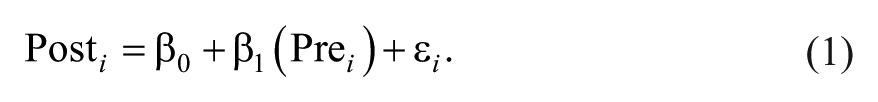
In Equation 1, the relationship between pretest scores and posttest scores is weighted based on the correlation between time points in the data (ultimately creating the regression coefficient β₁). In contrast, if difference scores were our outcome, we would have a formula like Equation 2A, with only an intercept (β₀) and an error term (εi):

$${\mathrm{Diff}}_i=\left({\mathrm{Post}}_i-{\mathrm{Pre}}_i\right)={\beta }_0+{\epsilon }_i.$$

(2A)

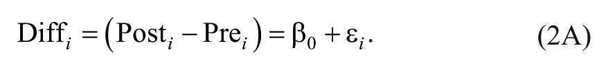
To see the correspondence between controlling for pretest as a covariate (Equation 1) and treating difference scores as an outcome (Equation 2A), we can simply move our pretest scores to the other side of the equal to sign (Equation 2B):

$${\mathrm{Post}}_i={\beta }_0+{\mathrm{Pre}}_i+{\epsilon }_i.$$

(2B)

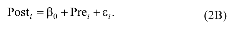
Note that there is no slope coefficient next to the pretest variable in Equation 2B, but the implied slope is 1. This slope is implied because in this equation, for every 1-unit change in pretest scores, we will have a 1-unit change in posttest scores (Equation 2B could be equivalently written as 1 × [Pre _i ]). Thus, using difference scores as our outcome is equivalent to assuming that the relationship between pretest and posttest scores is β₁ = 1.

Assuming a one-to-one relationship between pretest and posttest scores might be reasonable when the correlation between pretest and posttest score is very high, but in general, it is much better practice to control for pretest as a covariate. ²³ Controlling for pretest also allows for regression to the mean, whereas difference scores do not. That is, random error for lower-scoring participants is likely to drive their scores upward on a second measurement, and vice versa for high-scoring participants. Regression to the mean is less of a concern if we are dealing with clinical tests with high reliability (because measurement errors from test to test should be small). Even in that case, however, another benefit of controlling for pretest is that β₁ is weighted based on the correlation between pretest and posttest, whereas difference scores ignore this correlation. This is important because when the correlation between pretest and posttest is low, taking difference scores can actually add noise to the data. ⁹

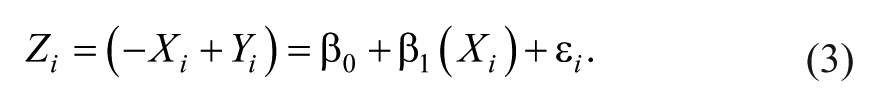
Thus, using change scores is already suboptimal, but the additional step of regressing change scores onto baseline measures leads to the issue of mathematical coupling discussed by Hawe et al ⁷ and Hope et al. ⁸ We illustrate the negative effects of mathematical coupling in Figure 1, using both a normal distribution (1A/B) and a uniform distribution with clear boundaries (1C/D; see Supplemental Appendix I for all simulation and analysis code.) The point of this illustration is to show that mathematical coupling is a different effect from boundaries on a scale, although the two can be related when floor/ceiling effects are present. In both simulations (n = 1000 data points), the variables X and Y are totally independent (r = 0.0). However, when we calculate a new variable Z = Y − X, we find that Z and X have a strong negative relationship (r = −0.7). The reason for this is that Z and X are mathematically “coupled”; that is, Z contains X, so they are intrinsically linked. This can be seen a little more clearly if we rearrange the terms for Z in a regression equation:

$$Z_i=\left(-X_i+Y_i\right)={\beta }_0+{\beta }_1\left(X_i\right)+{\epsilon }_i.$$

(3)

Figure 1.

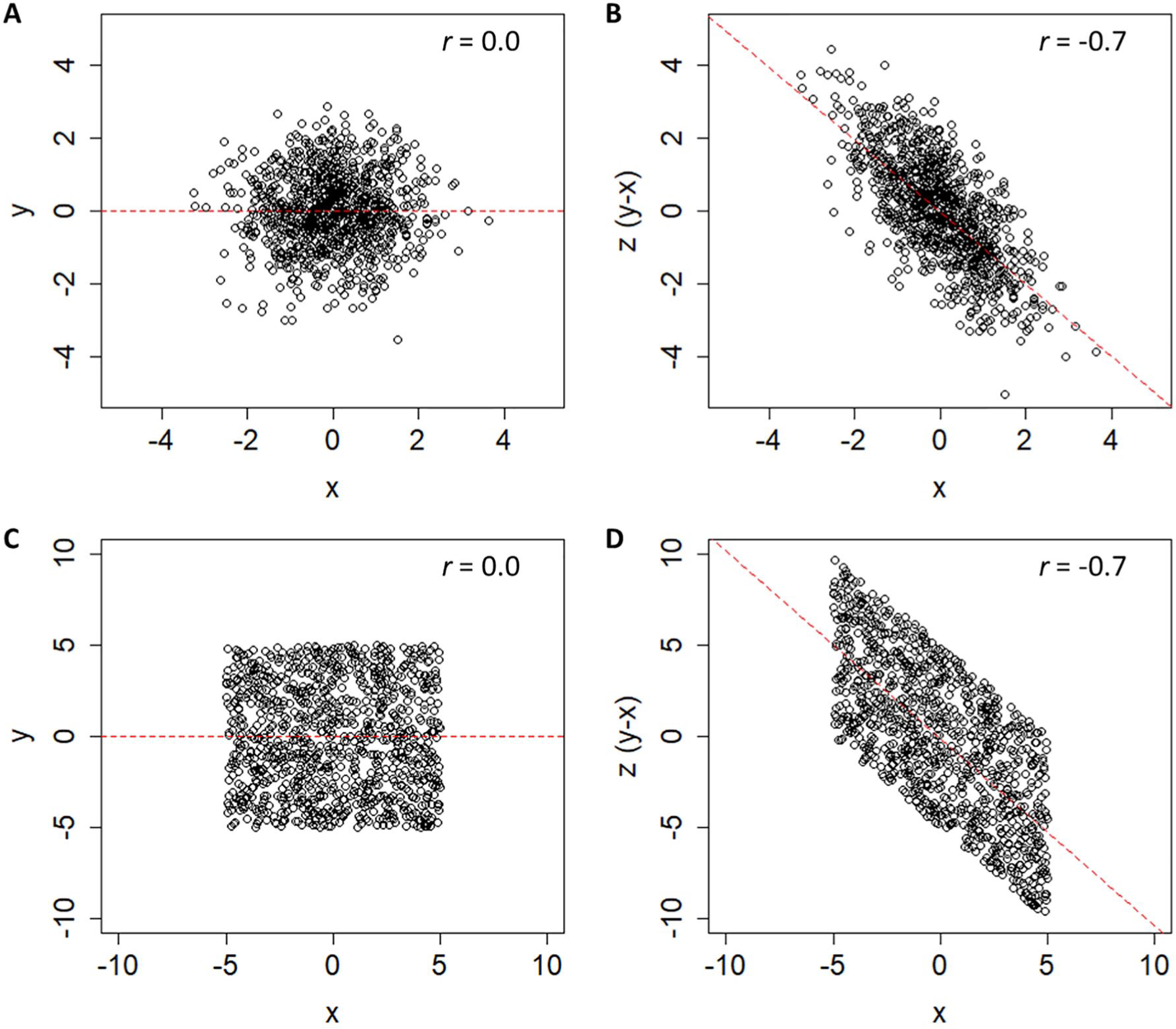
The n =1000 simulated data points showing 2 uncorrelated variables, X and Y, and a third variable Z, computed from their difference. In panels A and B, these variables are based on 2 normally distributed, but otherwise unbounded, distributions. In panels C and D, these variables are based on 2 uniform distributions with bounds of ±5. In both cases, an artifactual negative relationship exists between X and Z, because those values are mathematically coupled.

Because our change score (Z) is just our final score (Y) minus our initial score (−X), it is not surprising that −X and X are negatively related. In fact, the only thing distorting their relationship is Y. As Hope et al ⁸ pointed out, this is why the relative variance in X and Y matters. If the variance in Y is vastly smaller than X, we are essentially regressing −X onto X. If the variance in Y is vastly larger than X, we are essentially regressing Y onto X.

As such, it is generally bad practice to regress change scores onto baseline scores; doing so can lead to relationships that are artifacts resulting from mathematical coupling, rather than genuine relationships (for other medical examples, see Phang et al, ²⁴ Tu et al, ²⁵ and Browne et al ²⁶ ). Past critiques of proportional recovery have focused on the coupling that arises when change scores of the same variable are regressed onto baseline. However, it is important to point out that this coupling also arises if we regress change scores onto other values that are correlated with our baseline assessment. For instance, if we regressed change in the FMA onto baseline Action Research Arm Test (ARAT) scores and found a significant relationship, that relationship might still be a result of the fact that baseline FMA and ARAT scores are related, not because change in FMA is truly related to one’s baseline ARAT. Similarly, the same problem arises for CST integrity: CST integrity is related to baseline FMA, so some proportion of its relationship to change in FMA could also be a result of mathematical coupling.

Our comments thus far have focused on how mathematical coupling is a general concern any time change scores are regressed onto baseline characteristics. Now, we want to focus specifically on proportional recovery studies, where change in the FMA is regressed on baseline FMA scores. As shown in Figure 2, we have adapted the data gathered by Hawe et al. ⁷ These data reflect several different available studies on proportional recovery using the FMA.^{2,14,27 -30} Regressing the n = 373 change scores onto baseline levels of impairment shows an overall slope of 0.42 when the nonfitters (as identified in past studies) are included in the data. If these nonfitters are excluded, then the slope of the regression line is shifted upward, to 0.76 (as shown by a dashed black line in Figure 2). In either case, this slope is statistically different from zero; P values <.001. However, because of mathematical coupling, any relationship we find is either a statistical artifact or at least inflated by such an artifact. As such, we need to consider the adequacy of a traditional null-hypothesis test here.

Figure 2.

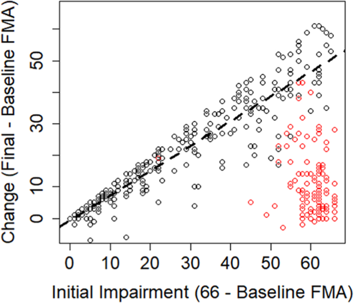
Data adapted from Hawe et al. ⁷ Change scores and initial impairments extracted from empirical studies have been combined to create an overall sense of the relationship across studies. The dashed line denotes the ordinary least-squared regression line for all fitters (black points). Data points that were identified as nonfitters in the original studies are shown as red points.

Consideration 2: Appropriate Null Hypotheses and Alternative Explanations

A common, null-hypothesis significance test for a regression slope assumes that the true value of the slope in the population is zero and that sampling variability is the only factor acting on the data. Other values can be chosen for the null hypothesis (eg, H₀: β = 0.5), but researchers often choose the nil-hypothesis significance test, where we explicitly assume that the true effect is zero (ie, the nil hypothesis is a specific case of the null hypothesis where H₀: β = 0, and for a 2-sided test, the alternative hypothesis would be H_a: β ≠ 0). As we have shown in the previous section (and as past work has shown in detail^7,8), it is not surprising to reject the nil hypothesis in this situation because of an artifact created by mathematical coupling. This artifact means that random sampling is not the only factor at work, nor should one expect a true relationship of zero, making the test of the nil hypothesis H₀: β = 0 uninformative.

It would, however, still be reasonable to ask if the observed relationship was greater than the mathematical artifact. This would require conducting a meaningful nonzero null-hypothesis test, and to do that, the mathematical artifact needs to be estimated. We will turn our attention more to that issue in consideration 3, but for now, let us consider 2 situations in which the nil hypothesis of β = 0 is rejected. In the first case (Figure 3A), we have simulated proportional recovery that leads to an average level of recovery of about 50% (ie, a regression slope of 0.50). In the second case (Figure 3B), we have simulated random uniform recovery, which will always lead to an average level of recovery of about 50% (because approximately half of the data will be below/above the mean change at each level of impairment).

Figure 3.

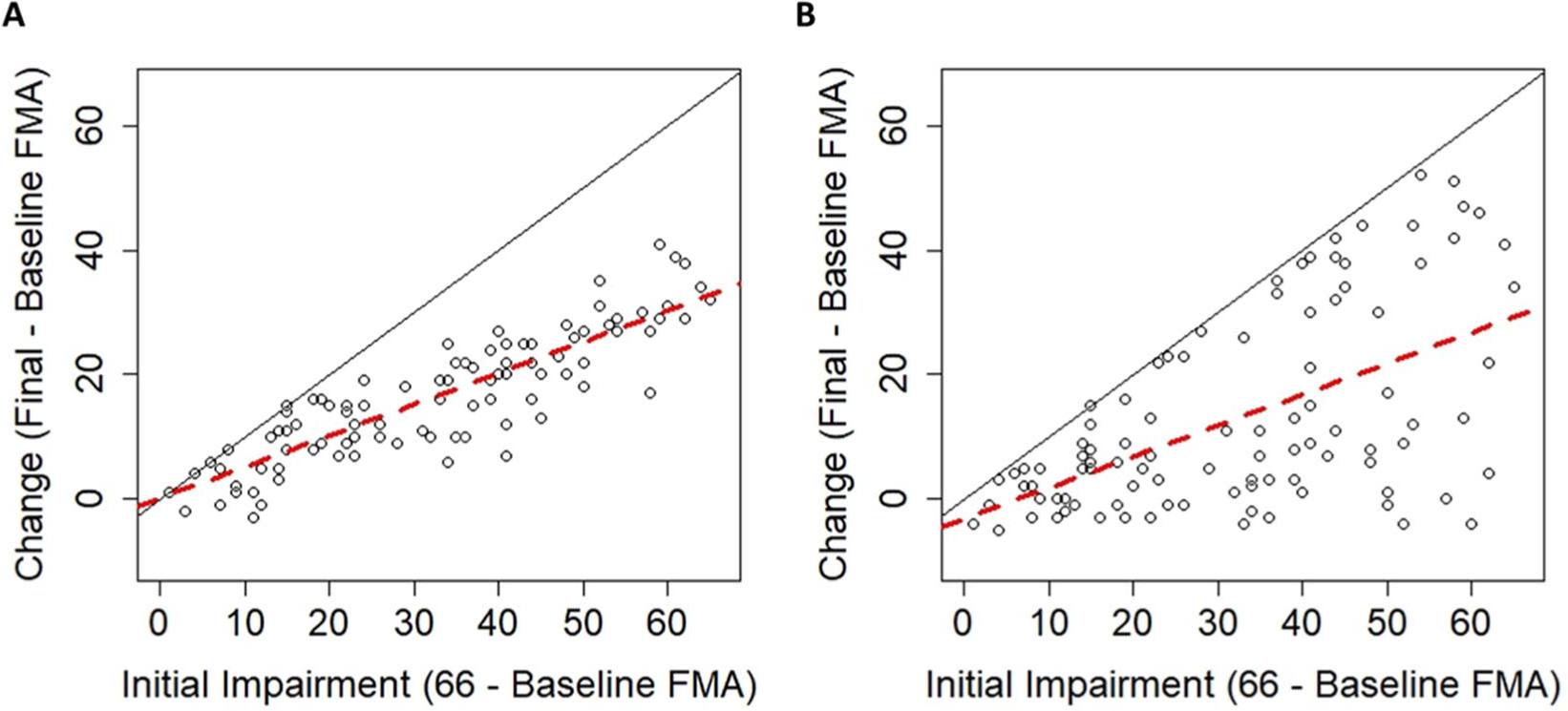
(A) Simulated data in which the change in Fugl-Meyer Assessment (FMA) is normally distributed around proportional recovery. (B) Simulated data in which the change in FMA follows a uniform distribution. In both cases, there is an upper bound on recovery because of the limits of the FMA (solid black lines), but even when change is random, there is a positive slope of ≈0.5 (dashed red lines).

For the proportional recovery example, data were normally distributed (σ = 6) around 50% of initial impairment, truncated by the ceiling of the FMA. Proportional recovery could be simulated with different parameters (eg, other means/SDs), but this is meant to be only 1 example of proportional recovery. For the random uniform example, data are uniformly distributed between a slight negative change (−6 points) and the maximum points allowed on the FMA (maximum possible recovery). Again, the uniform distribution could have different parameters, but this is meant to be only 1 example of random uniform recovery to illustrate our point.

Random uniform recovery is a reasonable distribution in this situation because it allows for the fact that different levels of recovery exist^15,31,32 but that the overall distribution of recovery can cover the entire available space. Patterns like uniform recovery have been shown in animal data^33,34 and human data using the FMA for the upper extremity, ¹⁹ the FMA for the lower extremity, ³ and the Arm Activity Measure. ³⁵ It is important to note that modeling recovery as random uniform change does not mean that recovery is an inherently random process; consistent, distinct patterns of recovery almost certainly exist ¹⁹ and are (at least) partially explained by physiological characteristics. ² Random uniform recovery simply assumes that the full space of recovery is possible and the distribution is uniform in the population (but, naturally, this will vary from sample to sample).

As we have shown, a proportional looking relationship already exists at the group level whether recovery is proportional or uniform. In both cases in Figure 3, the regression slopes would suggest that recovery is about 50% proportional and we would reject the nil hypothesis (H₀: β = 0) in each case (proportional case: b = 0.50, P < .001; uniform case: b = 0.49, P < .001). Comparing the plots in Figure 3 helps illustrate that rejecting this null hypothesis does not mean that a particular explanation for the effect is correct; it merely means that the data were unlikely to have arisen if the null were true. That is, we reject the null hypothesis, H₀: β = 0, and we are inclined to accept the alternative, H_a: β ≠ 0. However, rejecting the null does not imply that a particular scientific theory/explanation/hypothesis is true.

An important part of the proportionality argument is how individual changes are distributed around the group-level slope. If everyone is clustered around the group-level slope (Figure 3A), then the proportional argument seems very reasonable. Conversely, if everyone can be distributed across the entire space of recovery (Figure 3B), then we think this association is a statistical artifact. Contrasting the empirical data from Figure 2 against the simulated data in Figure 3, that conclusion crucially depends on whether or not nonfitters are included in the sample. In Consideration 3, we explore the validity of the fitters classification by showing how hierarchical clustering procedures lead to the spurious identification of nonfitters even when recovery follows a random uniform distribution. Furthermore, in Supplemental Appendix II, we present analyses of the variability in the real data (n = 373 shown in Figure 2) at different levels of initial impairment. In brief, those analyses show that the variance at most levels of initial impairment is not statistically different from random uniform recovery, but there are pockets of impairment levels where recovery shows less variance than expected.

Together, the simulation results raise questions about the validity of the fitters classification, and the variance analyses suggest that real individual changes are not reliably different from uniform recovery at most levels of initial impairment (with notable exceptions in the middle of the distribution). Before we address those concerns, it is important to clarify what we mean by group-level statistics and individual-level data. As Kundert et al ⁴ write in their abstract, “existing data are largely consistent with the [proportional recovery rule] at the population-level, . . . recent reports of its demise are exaggerated, as they excessively focus on the less conclusive issue of individual subject-level predictions (p. 876).”

When we are discussing individual-level data in this perspective, we mean how classification of individuals into fitters and nonfitters ultimately affects the group-/population-level statistics we observe when the data are aggregated. The decision about proportionality depends on how individuals spread around the group-level slope. Thus, the validity of excluding nonfitters is a critical issue. However, by individual-level, we do not mean making specific predictions about how an individual recovers. In the examples we have discussed so far, initial impairment is associated with/explains variance in change scores. We reserve the word prediction to refer specifically to the classification of individuals in independent samples (eg, PREP ³⁶ or TWIST algorithms ³⁷ ). This sort of out-of-sample individual prediction was not the original purpose of the proportional recovery rule, nor is it part of our critique.

Consideration 3: Measurement Issues Can Create the Illusion of Proportionality

The fact that proportional recovery is apparent across many different scales of measurement has been argued as evidence for proportional recovery being a neurobiological phenomenon. ⁴ First shown in the FMA, ¹ proportional recovery has since been shown in the Functional Independence Measure, ⁷ the Western Aphasia Battery, ³⁸ and the Letter Cancellation Test, ³⁹ among other inventories. However, all these inventories possess lower and upper bounds. Although the individual minima and maxima are all different, the presence of these boundaries creates a real problem for interpreting the relationship between baseline scores and change scores. The code provided in the Supplemental Appendix I can be revised to demonstrate this point, but one can also consider Figure 3B in a thought experiment. Regardless of what the individual minima and maxima of these different scales are, random uniform recovery will always lead to the bottom triangle of the possible space being covered.

As shown in Figure 2, however, we can see that the story is more complicated than that because the distribution of initial impairments for the FMA is not uniform. There are higher densities of very low and very high impairments on the FMA. Therefore, to make our simulations ⁴⁰ more realistic, we bootstrapped (ie, repeatedly sampled) the initial impairment data from Hawe et al ⁷ (shown in Figure 2) to get a new “population” of 10 000 initial impairments with a similar distribution of initial impairments but uniformly distributed change scores.

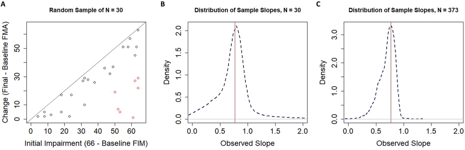
Using this simulated population, we can repeatedly draw samples to see how the data look from one sample to the next. One such sample of n =30 participants is shown in Figure 4A. The regression slope in this sample happens to be β = 0.62, as shown by the dashed red line. Taking repeated samples, however, leads to a distribution of sample slopes as shown in Figure 4B. The dashed blue line shows the distribution of sample slopes from k =10 000 independent samples. As discussed above, these slopes vary around a population-level slope of β =0.50 purely as a result of the mathematical artifact of regressing change scores onto initial impairments. Thus, to decide if our single-sample slope of 0.62 is interesting, we need to take this mathematical artifact into account. As shown in Figure 4C, the slope of 0.62 is statistically surprising under the nil hypothesis of no effect (P < .001; the dashed black line centered on 0) but is no longer statistically surprising when the null hypothesis takes the mathematical artifact from random uniform recovery into account (P = .337; the dashed blue line centered on 0.5). Large positive associations between change and initial impairment should be expected, not because of any inherent biological correspondence but because of how we handled the data.

Figure 4.

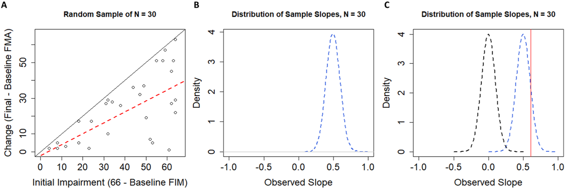
A. A single random sample of n =30 FMA scores drawn from our population. The regression line (dashed red) has a slope of 0.62, which might suggest proportional recovery were it not drawn from a sample of randomly generated data. A diagonal black line with a slope of 1 is shown for reference. B. The sampling distribution of slopes when our simulated population was sampled 10 000 times, with replacement, at sample sizes of n =30. C. Contrasting the distribution of sample slopes under the nil-hypothesis H₀: β = 0 (dashed black line) and the distribution of sample slopes from our simulated population (centered on 0.5; dashed blue line). Note that now our observed slope of 0.62 (shown as the vertical red line) is no longer statistically significant when we use a null hypothesis that takes the mathematical artifact into account (P <.001, when H₀: β = 0, vs P =.337 when H₀: β = 0.5).

At this point, it is critical to consider the exclusion of nonfitters, because that is how data are handled in proportional recovery studies. Methods that have been used to distinguish fitters from nonfitters can be legitimate methods whether they are data-driven methods (such as hierarchical cluster analysis) or theory-driven methods (such as moderator analyses using physiological data^2,15). We are not debating the fundamental accuracy of these approaches, but their use in the classification of fitters and nonfitters in this context.

To address the validity of hierarchical clustering as a method for classifying individuals as fitters or nonfitters, we will use our simulated population of individuals with random uniform change scores. In the first run of our simulations, we took k =10 000 samples of n =30 individuals. In each sample, we used hierarchical cluster analysis^40,41 to identify clusters of participants who could be classified as fitters and nonfitters. As shown in Figure 5A, the clustering algorithm still identifies clusters of participants as fitters (black dots) and nonfitters (red dots) when sampling from data with random uniform change scores. Obtaining clusters of fitters and nonfitters is obviously problematic in this case because the underlying change is uniform. As such, we should be concerned that fitters and nonfitters may be (at least partially) an artifactual classification.

Figure 5.

A. A single random sample of n =30 participants drawn from a population with random change scores. Note that the clustering algorithm still classifies participants into what look like fitters and nonfitters even when there is no rule to which individuals can fit. B. The distribution of sample slopes for fitters identified by our clustering procedure when the original sample size was n =30. C. The distribution of sample slopes for fitters identified by our clustering procedure when the original sample size was n =373.

Current procedures described in studies of proportional recovery are not entirely clear on how their clusters were ascertained. That is, a cluster analysis can work using either a bottom-up agglomerative procedure or a top-down divisive procedure, but in general, authors have an objective criterion for where they stop in determining their clusters. Although it has been stated that a criterion has been used, ²⁸ it is not clear what the numerical value of this criterion is.^2,29,38 As such, it is not clear by what criteria authors are making the decision to stop at 2 clusters in their analyses. We do know that authors are calculating Mahalanobis distances between points ⁴² and that these distance values are being used as input into the agglomerative clustering algorithm advocated by other authors ⁴¹ and Ward. ⁴³ In the absence of a clear criterion by which we should stop clustering, we ran cluster analyses in our simulations that always stopped at 2 clusters. To determine which cluster was the fitters, we chose the cluster with a higher mean change score (consistent with the central argument of proportional recovery). Otherwise, our simulations used methods identical to published work for calculating distances and determining clusters.

As shown in Figure 5A, our clustering procedure leads to an identification of fitters (black dots) and nonfitters (red dots) to the proportional recovery rule consistent with past literature, despite coming from a population of random uniform recovery. This result is likely a result of the asymmetry in the variable space. That is, when empirical and predicted change scores are fed into the algorithm, major deviations from the predicted change can only occur in the negative direction (lower right corner of Figure 5A), because individuals cannot improve beyond the maximum score of the scale (represented by the solid black line in Figure 5A). We show the effects of this procedure (sampling, clustering, and estimating slopes for the fitters’ cluster) when the total size is n =30 (to illustrate a relatively small, but common sample size) and when the total n =373, matching the total sample size for the pooled data. ⁷

As shown in Figure 5B, when we simulated samples of size n =30, the distribution of sample slopes for the fitters had a mean of 0.770, a median of 0.781, and a negative skew. Thus, under this sampling distribution, we would not find it surprising to observe a large positive slope of 0.769 (as was observed in Hawe et al ⁷ ). Specifically, with a starting sample size of n =30, we would expect a slope of ≥0.769 for the fitters about 54% of the time.

We reach a similar conclusion if we take the pooled real data for the fitters. The slope for the n =254 fitters out of those initial n =373 participants was 0.769. ⁷ As shown in Figure 5C, simulating random uniform recovery, hierarchical cluster analysis with 2 clusters, and that fitters would be the group with higher mean change, the mean of this sampling distribution was 0.778 and the median was 0.771. Based on this simulated distribution, we would expect to get a slope of ≥0.769 for the fitters about 54% of the time.

Our simulated data (assuming random uniform recovery) led to a similar classification of fitters and nonfitters when fed into hierarchical clustering algorithms (see Supplemental Appendix II for more details about these clusters). This finding casts doubt on the validity of the fitters classification, because in the simulations, there is no proportional recovery rule to which an individual can fit. This result suggests that the fitters classification is (at least in part) artifactual. This spurious classification is a new finding and has important implications for how we should interpret other results.

First, data invoked as evidence for the proportional recovery rule are relatively weak. These patterns are quite consistent with what one might expect if recovery was uniformly and randomly distributed. Kundert et al ⁴ are quite correct when they wrote, “The fact that one can generate data that reproduces some findings of the PRR does not mean that the [proportional recovery rule] is invalid or that the observed data does not represent biologically meaningful associations (p. 884).” However, if we had a null-hypothesis test P value of .54, we would not reject the null hypothesis. Proportional recovery is no different. We have shown that the group-level slope of b = 0.769 carries a P =.54 for fitters based on a sample of n =373 when we assume random uniform recovery. As such, we should not reject the hypothesis that recovery is uniformly distributed, nor should we accept the hypothesis that recovery is proportional at this time. Current data are consistent with both hypotheses, but the methods of measurement and analysis are rife with statistical limitations. Thus, we argue for abandoning current approaches to measuring proportional recovery, and we would generally caution against measuring recovery as the difference between 2 time points.

Second, studies showing that physiological characteristics are associated with the fitters/nonfitters classification should instead be reframed as physiological characteristics associated with important variation in recovery. For instance, individuals with poor CST integrity are not “nonfitters”, but they are more likely to have significant impairment and poor recovery. ² The integrity of specific brain regions clearly plays an important role in the potential for recovery. There is, however, still substantial variability even among neuroanatomically similar individuals. ³² Recovery is a complex and multivariable problem, and the field still has much work to do explaining individual differences in recovery trajectories.

Discussion

The proportional recovery rule has been an influential finding in the field of neurorehabilitation. Recent debates about its accuracy and validity are also a very useful case study, highlighting more general concerns for the study of recovery. Data argued to show proportional recovery in stroke rehabilitation have been found across a wide variety of assessments and replicated in many different samples. This pattern appeared so pervasive and the relationship so strong that it was compelling to think of this pattern as a neurological rule. As we have shown, however, current patterns claimed to be evidence for proportional recovery are generally consistent with uniform random recovery in these measures. This does not mean that proportional recovery has been disproven, but it does mean that we do not have the data to reliably say that recovery is proportional at this time.

Combining our simulations with analyses of the variance in the real data, our results cast doubt on the nonfitters classification and suggest that variability in recovery is greater than what has been suggested by the proportional recovery rule. However, we also do not conclude that recovery is uniformly distributed across all levels of impairment (or for all measures). Indeed, as shown in Supplemental Appendix II, there are some levels of initial impairment where variance in change scores is lower than would be expected under random uniform recovery for the FMA. Thus, it is very likely that there are nonuniformities, but it is not clear from the current data if this is a result of nonlinearities in the FMA. Ultimately, whether recovery is (partly) proportional or not, the methods commonly used to support proportional recovery are flawed, and future arguments for (or against!) proportional recovery need to be based on different methods and data.

It is also important to remember that whether variation is uniform or not, the variation is not pure chance; it is uncertainty that needs to be explained. There is very compelling evidence that physiological variables explain individual differences in recovery, ²² but this is a very different question from claiming that recovery is proportional and that there are nonfitters to this general rule. As our simulations show, clusters of fitters and nonfitters emerge even when recovery is uniformly distributed. Thus, rather than concluding that individuals with lower CST integrity are more likely to be nonfitters, we think that a more appropriate conclusion is that individuals with lower CST integrity are likely to be severely impaired and to show minimal recovery. That is, we need to think about recovery more continuously and less dichotomously. There are reliable individual differences in recovery, and people with more similar neuroanatomy following stroke are likely to show more similar patterns of recovery (although there is still variation in recovery trajectories for neuroanatomically similar individuals ³² ).

Limitations in Our Simulations

Our simulations used an empirical distribution of initial impairment values, but they assumed a uniform distribution of change scores for any given level of impairment. One could question the appropriateness of assuming random uniform change at all, but especially in the context of the FMA upper-extremity subscale. Visually, there appears to be an “island” of severely impaired individuals in the empirical data shown in Figure 2. This island is (at least) partially created by nonlinearities in the FMA.^6,7 Specifically, midrange scores are less likely to occur in the FMA upper extremity subscale. If these midlevel scores are less likely, it makes sense that moderately impaired individuals will progress out of this range but severely impaired individuals will be more likely to either surpass it or struggle to get into it (creating the island of nonfitters). Hawe et al ⁷ took this bimodal distribution of change scores into account in their simulations, but in the current study, we explicitly chose to model change uniformly for 4 reasons.

First, the artifacts that are generated by regressing bounded change scores onto baseline scores are not a product of this nonlinearity (as shown in our simulations). Nonlinearity is a special concern for certain scales, but the problems created by ceiling/floor effects are more general. Second, data from both animal and human studies suggest that more uniform patterns of recovery exist for a variety of scales.^3,19,33,39 As such, uniform random recovery is a valid null hypothesis against which to test. Third, assuming uniform random recovery illustrates how hierarchical cluster analysis with Mahalanobis distances can break down in this situation. When pairwise distances are calculated based on predicted change and actual change, these cluster analyses will spuriously identify fitters and nonfitters.* Fourth, as shown in Supplemental Appendix II, this island is much less pronounced when recovery is normalized to the level of initial impairment and the observed variances in the real data are not statistically different from random uniform recovery, at most levels of initial impairment.

Beyond Proportional Recovery

The debate around proportional recovery also highlights questions about design, measurement, and statistical analysis that are broadly important to clinicians/researchers:

• First, when designing a study, it is important to decide if our focus is on end points or trajectories. If our focus is on end points, then end points should be our outcome, and we should control for baseline measures as covariates. Conceptually, this is more like Figure 6A, where we show the cumulative data from Hawe et al. ⁷ Rather than plotting change as a function of initial impairment, we are now showing final FMA upper extremity scores as a function of baseline scores. If our focus is on trajectories, however, then we need to model change over time, more like Figure 6B. As we have shown, however, the distinction between fitters and nonfitters is, at least in part, an artificial classification, and there could be many more groups that make up the possible recovery space, as shown conceptually in Figure 6C. To reliably model these longitudinal trajectories, however (eg, in latent growth curve models, multilevel models), we need more than 2 data points. An advantage of these models is that they can avoid issues of mathematical coupling because the model estimates a trajectory rather than regressing change scores onto baseline variables. This is very much the technique adopted by van der Vliet et al, ¹⁹ who used longitudinal mixture models to identify 5 subgroups of participants with a mean of 6.1 measurements per person. The insights gleaned from their longitudinal study show the power of these approaches, and we very much recommend these types of models (or similar^18,44,45) as the field moves forward.

• Second, it is important to remember that the null-hypothesis significance test answers a single, very specific question^46,47: “Assuming all our assumptions are correct (the true effect is some specific value [often zero], sampling variability is the only factor acting on our data, etc), what is the probability of observing data this extreme or more extreme?” Rejecting the null hypothesis means that we accept the alternative hypothesis in a statistical sense (ie, we reject H₀: β = 0 to favor H_a: β ≠ 0), but it does not mean that a particular explanation of the effect is correct, and we need to carefully consider how to choose between alternative explanations when the null is rejected.

• Third, it is important to avoid subgrouping the data in an arbitrary manner. Post hoc segregation of change scores into fitters and nonfitters echoes similar pursuits like classifying responders and nonresponders based on distributions of change scores ⁴⁸ and is similarly problematic. ⁴⁹ Classifying individual responses to treatment is a very difficult proposition, and it must be done carefully. Indeed, in most clinical trials, it might not even be possible. ⁵⁰ That said, we also should not ignore reliable subgroups/individual differences that are supported by outside information. Meaningful differences in recovery and initial impairment are related physiological variables^5,15 and specific behavioral tests. ⁶ However, we stress again that these relationships are not evidence for nonfitters to an otherwise pervasive rule; we should think about recovery and impairment more continuously, with anatomy/physiology explaining important variation.

• Fourth, and finally, it is important to consider the properties (and limitations) of the scales that we are using to quantify recovery. Many clinical scales have strong ceiling/floor effects because healthy (“normal”) performance is the maximum/minimum against which performance is being measured. Although this is a reasonable choice for scale design, we need to be very cautious about the effects of these boundaries.^7,8 Additionally, many clinical scales produce ordinal data, but we often treat these data as interval/ratio data (especially when aggregated). For instance, a +2-point change on the FMA could be the result of a single 2-point change in elbow extension or two 1-point changes in shoulder flexion and pronation-supination. Thus, higher FMA scores generally mean less impairment, but 2 people with the same FMA score do not necessarily have the same impairment, nor do differences in FMA scores always mean the same change in impairment. Treating ordinal data as interval data is not always a problem, ⁵¹ and there are times we might actually transform ordinal data into interval data, ⁵² but we always need to carefully consider the pros and cons of how we choose to measure “recovery.”

Figure 6.

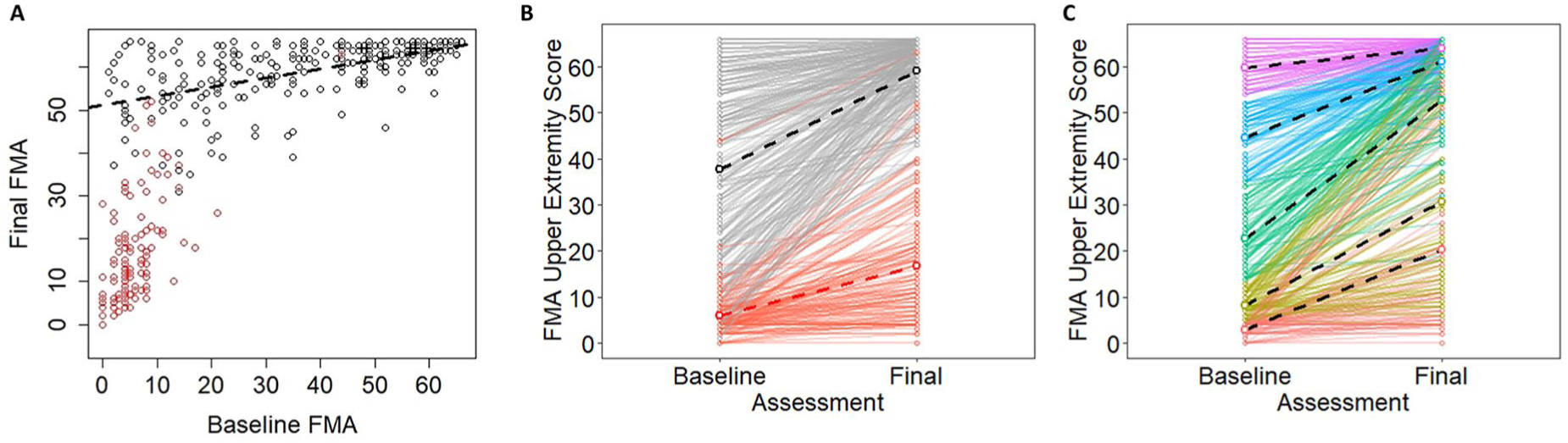
A. Pooled empirical data from Hawe et al ⁷ shown as a function of baseline Fugl-Meyer Assessment (FMA) scores. B. The same data shown as trajectories for individual participants over time. Note that black dots correspond to fitters and red dots correspond to nonfitters in their original classifications. C. A conceptual model in which the same data are color coded based on quintiles of the baseline scores. Dashed lines show best fitting regression slopes within the various subgroups.

Conclusions

Our goal in this point of view was to provide a checklist of conceptual and analytical issues in longitudinal measures of stroke recovery. We used proportional recovery as an illustrative example, but these issues of design, measurement, and analysis are broadly important for neurorehabilitation researchers. Using simulations, we showed the following: (1) how change scores can be problematic in this context; (2) how “nil” and nonzero null-hypothesis significance tests can be used and interpreted; and (3) how scale boundaries can create the illusion of proportionality (eg, floor/ceiling effects), whereas other analytical procedures (eg, spurious identification of nonfitters/nonresponders) can augment this problem. Moving forward, understanding of the recovery process will be enhanced by embracing alternative designs (eg, with more data collections at critical time points), using different methods of analysis (eg, that model true longitudinal trajectories), and exploring new outcome measures (eg, that avoid the ceiling effects of ordinal, criterion-based scales).

Supplemental Material

sj-pdf-1-nnr-10.1177_1545968320975437 – Supplemental material for Statistical Considerations for Drawing Conclusions About Recovery

Supplemental material, sj-pdf-1-nnr-10.1177_1545968320975437 for Statistical Considerations for Drawing Conclusions About Recovery by Keith R. Lohse, Rachel L. Hawe, Sean P. Dukelow and Stephen H. Scott in Neurorehabilitation and Neural Repair

Supplemental Material

sj-pdf-2-nnr-10.1177_1545968320975437 – Supplemental material for Statistical Considerations for Drawing Conclusions About Recovery

Supplemental material, sj-pdf-2-nnr-10.1177_1545968320975437 for Statistical Considerations for Drawing Conclusions About Recovery by Keith R. Lohse, Rachel L. Hawe, Sean P. Dukelow and Stephen H. Scott in Neurorehabilitation and Neural Repair