The beyondpareto command for optimal extreme-value index estimation

Abstract

In this article, we introduce the command beyondpareto, which estimates the extreme-value index for distributions that are Pareto-like, that is, whose upper tails are regularly varying and eventually become Pareto. The estimation is based on rank-size regressions, and the threshold value for the upper-order statistics included in the final regression is determined optimally by minimizing the asymptotic mean squared error. An essential diagnostic tool for evaluating the fit of the estimated extrerme-value index is the Pareto quantile–quantile plot, provided in the accompanying command pqqplot. The usefulness of our estimation approach is illustrated in several real-world examples focusing on the upper tail of German wealth and city-size distributions.

1 Introduction

Many distributions in economics and the natural sciences exhibit upper tails that decay like power functions. In economics, leading cases of interest are the upper tails of the wealth and income distributions in the inequality literature, of the city-size distribution in urban economics, and of the firm-size distribution in industrial economics (see, for example, the discussion in Schluter and Trede [2019] and references therein). Outside of economics, other size distributions of interest (among many others) are internet traffic, word frequencies, or biological systems.

More specifically, let the cumulative distribution function F be regularly varying, so for sufficiently large y,

$$F(y)=1-y^{-1/\gamma }l(y)(\gamma >0)(1)$$

(1)

where l denotes a slowly varying nuisance function that is constant asymptotically $[l(ty)/l(y)=1\mathrm{as}y\to \mathrm{\infty }]$ . $\gamma >0$ is called the extreme-value index, and the Pareto or tail index ( $\alpha \equiv 1/\gamma$ ) is its reciprocal. The objective is to estimate the parameter $\gamma$ . A popular approach is to assume that the tail of F is exactly or generalized Pareto beyond a fixed threshold value and then to use maximum likelihood (see, for example, Jenkins [2017] and Charpentier and Flachaire [2022]).¹ The question of where the Pareto tail starts is usually not addressed explicitly; the two articles cited earlier are notable exceptions. However, the empirical challenges are that real-world size distributions are rarely exactly Pareto and that convergence to the Pareto can be slow. Such slow convergence will be manifested in the Pareto quantile–quantile (QQ) plot, which becomes linear only eventually. If the choice of the threshold value falls in the nonlinear part of the plot, the estimator of $\gamma$ will be distorted. Schluter (2018, 2021) demonstrates that these distortions can be considerable. In particular, the Pareto QQ plot tends to exhibit a concavelike curvature that ultimately leads to an overestimate of $\gamma$ .

While many estimators of the extreme-value index are proposed in the statistical literature (see, for example, the textbook treatments in Embrechts, Klüppelberg, and Mikosch [1997] and Beirlant et al. [2004]), we consider here the rank-size regression estimator because of its popularity among applied researchers (see, for example, Atkinson [2017] and the reference therein for the inequality literature, and see Schluter [2021] for the city-size literature).² In some literature, this regression is referred to as a Zipf regression, and some controversies center on whether $\gamma$ is equal to unity or simply positive or whether the size distribution is lognormal or Pareto-like (these are discussed extensively in Schluter and Trede [2019]).³

Schluter (2018) provides the distributional theory for the rank-size regression estimator in the distributional model (1) and considers an optimal data-dependent threshold choice based on the minimization of the asymptotic mean squared error (AMSE). Schluter (2021) discusses in detail the usefulness of the Pareto QQ plot as a diagnostic tool, while König, Schluter, and Schröder (2023) have generalized the procedure to accommodate complex survey design. These articles also provide applications to the upper tails of the wealth, income, and city-size distributions. The command beyondpareto implements these estimation and inference procedures. The accompanying command pqqplot produces Pareto QQ plots to visually assess the fit of the Pareto distribution for different cutoff values. Later sections provide real-world illustrations of the usefulness of these techniques, some of which are included in the help files.

2 Statistical theory

The rank-size regression estimator of the extreme-value index measures the ultimate slope of the Pareto QQ plot. This follows because the tail quantile function for model (1) is $U(y)=\inf \{t:\mathrm{Pr}(Y>t)=1/y\}=y^{\gamma }\stackrel{\sim }{l}(y)$ , where $\stackrel{\sim }{l}(y)$ is a slowly varying function, which then implies $\log U(y)\sim \gamma \log (y)$ as $y\to \mathrm{\infty }$ . Replacing these population quantities with their empirical counterparts gives the Pareto QQ plot, and $\gamma$ is its ultimate slope. If the tail of the distribution were strictly Pareto, then the Pareto QQ plot would be linear, and a linear regression would estimate its slope coefficient. In model (1), it will become linear only eventually, and a slow decay of the nuisance functions $l(y)$ and $\stackrel{\sim }{l}(y)$ will then induce asymptotic distortions in the estimator of the slope coefficient. Below such slow convergence will be considered in the form of second-order regular variation.⁴

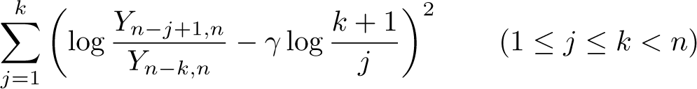
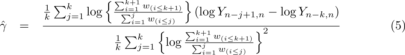
Let $Y_{1,n}\le \cdots \le Y_{n,n}$ denote the order statistics of the given sample $Y_1,\dots ,Y_n$ of for example, wealth or income, and consider the k upper-order statistics. The Pareto QQ plot has coordinates $(-\log \{j/(n+1)\},\log Y_{n-j+1,n}{)}_{j=1,\dots ,k}$ , where the relative rank is given by $-\log \{j/(n+1)\}$ and $j=1$ for the highest upper-order statistic. The ordinary least-squares estimator of the slope parameter in the Pareto QQ plot is obtained by minimizing the least-squares criterion

$$\sum _{j=1}^k{\left(\log {\displaystyle \frac{Y_{n-j+1,n}}{Y_{n-k,n}}-\gamma \log {\displaystyle \frac{k+1}{j}}}\right)}^2(1\le j\le k<n)$$

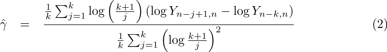
with respect to $\gamma$ , which corresponds to a regression of log sizes on the log of relative ranks for sufficiently large values given by $Y_{n-k,n}$ . Note that $Y_{n-j+1,n}/Y_{n-k,n}$ is a normalized size equal to 1 at the threshold. The resulting ordinary least-squares estimator is

$$\begin{array}{ccc}\hat{\gamma }& & ={\displaystyle \frac{{\displaystyle \frac{1}{k}{\sum }_{j=1}^k\log \left({\displaystyle \frac{k+1}{j}}\right)(\log Y_{n-j+1,n}-\log Y_{n-k,n})}}{{\displaystyle \frac{1}{k}{\sum }_{j=1}^k{\left(\log {\displaystyle \frac{k+1}{j}}\right)}^2}}}\end{array}(2)$$

(2)

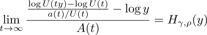
The distributional theory for $\tilde{\gamma }$ requires imposing more structure on the behavior of nuisance functions. It is common practice in the extreme-value literature to strengthen the first-order regular representation to second-order regular variation. Recall that model (1) has the equivalent (first-order regular variation) representation ${\lim }_{t\to \mathrm{\infty }}\{\log U(ty)-\log U(t)\}/\{a(t)/U(t)\}=\log y$ , where a is a positive norming function with the property $a(t)/U(t)\to \gamma$ . We then assume that

$$\underset{t\to \mathrm{\infty }}{\lim }{\displaystyle \frac{{\displaystyle \frac{\log U(ty)-\log U(t)}{a(t)/U(t)}-\log y}}{A(t)}=H_{\gamma ,\rho }(y)}$$

for all $y>0$ , where $H_{\gamma >0,\rho <0}(y)=1/\rho \{(y^{\rho }-1)/\rho -\log y\}$ with $\rho <0$ . The parameter $\rho$ is the so-called second-order parameter of regular variation, and $A(t)$ is a rate function that is regularly varying with index $\rho$ ，with $A(t)\to 0$ as $t\to \mathrm{\infty }$ . As $\rho$ falls in magnitude the nuisance part of l in (1) decays more slowly. Many heavy-tailed distributions satisfy this second-order representation, such as members of the Hall class of distributions given by $F(x)=1-a{x}^{-1/\gamma }\{1+b{x}^{\beta }+o(x^{\beta })\}$ for large values of x, whose tail quantile function is $U(x)=c{x}^{\gamma }\{1+d{x}^{\rho }+o(x^{\rho })\}$ .

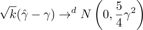
Schluter (2018) then demonstrates that as $k\to \mathrm{\infty }$ and $k/n\to 0$ , this estimator is weakly consistent, and if $\sqrt{k}A(n/k)\to 0$ ,

$$\sqrt{k}(\hat{\gamma }-\gamma ){\to }^{d}N\left(0,{\displaystyle \frac{5}{4}{\gamma }^2}\right)$$

Asymptotically, the estimator is thus unbiased if $\sqrt{k}A(n/k)\to 0$ . But if this decay is slow, the estimator will suffer from a higher-order distortion in finite samples given by

$$b_{k,n}\equiv {\displaystyle \frac{1}{2}{\displaystyle \frac{\gamma }{\rho }{\displaystyle \frac{2-\rho }{{(1-\rho )}^2}A(n/k)(\gamma >0,\rho <0)}}}$$

2.1 The choice of the threshold k for the upper-order statistics

Any tail index estimator requires a choice of how many upper-order statistics, given by k, should be accounted for. This choice invariably introduces a tradeoff between bias and precision of the estimator that is typically ignored by practitioners. However, this mean-variance tradeoff suggests that it is unwise to set the threshold level mechanically (for example, a wealth level of 1 million euros or $10\text{\%}$ of the sample). By contrast, we determine this threshold level in a data-dependent manner for estimator (2) by using the residuals in the rank-size regression to nonparametrically estimate the amse.

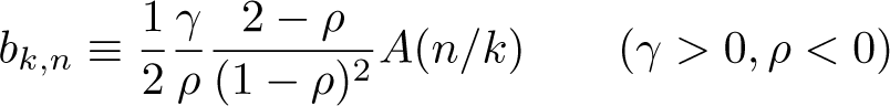
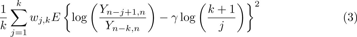
Following Beirlant, Vynckier, and Teugels (1996) and Schluter (2018, 2021), we observe that the expectation of the mean-weighted theoretical squared deviation

$${\displaystyle \frac{1}{k}\sum _{j=1}^k{w}_{j,k}E{\left\{\log \left({\displaystyle \frac{Y_{n-j+1,n}}{Y_{n-k,n}}}\right)-\gamma \log \left({\displaystyle \frac{k+1}{j}}\right)\right\}}^2(3)}$$

(3)

equals, to first order, $c_k\mathrm{Var}(\hat{\gamma })+d_k(\rho )b_{k,n}^2$ for some coefficients $c_k$ depending only on k and for $d_k(\rho )$ depending on k and $\rho <0$ . For an explicit statement of the coefficients $c_k$ and $d_k$ , see Schluter (2018). The procedure then consists of applying two different weighting schemes $w_{j,k}^{(i)}(i=1,2)$ in (3), estimating the corresponding two mean-weighted theoretical deviations using the residuals of regression (2), and computing a linear combination thereof such that $\mathrm{Var}(\hat{\gamma })+b_{k,n}^2$ obtains. We proceed in this manner for weights $w_{j,k}^{(1)}\equiv 1$ and $w_{j,k}^{(2)}=j/(k+1)$ for a set of preselected values of $\rho$ . In particular, based on the experiments reported in Schluter (2018, 2021), we have set a very conservative value of $\rho =-0.5$ (implying a slow decay of the slowly varying nuisance function $l$ ).

2.2 Complex surveys

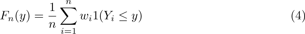
Survey data often come with sampling weights to allow inference on the level of the population. The aforementioned theory and methods are easily adapted to this setting if we define the weighted empirical distribution function as

$$F_n(y)={\displaystyle \frac{1}{n}\sum _{i=1}^n{w}_{i}1(Y_i\le y)(4)}$$

(4)

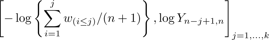
where $w_i$ is the sampling weight associated with the ith observation $Y_i$ with ${\sum }_{i=1}^n{w}_i=n$ . Examples are a scheme of unity weights ( $w_i\equiv 1$ for all $\dot{i}$ ) or $w_i=\widetilde{w_i}n$ with $0<{\tilde{w}}_i<1$ and ${\sum }_i{\tilde{w}}_i=1$ . Then, for the jth largest observation, we have $F_n\{Y_{n-(j-1),n}\}=\left(n-{\sum }_{i=1}^j{w}_{(i\le j)}\right)/n$ with the implicit notation convention that ${\sum }_{i=1}^j{w}_{(i\le j)}$ denotes the summation of the survey weights corresponding to the j largest upper-order statistics. The resulting Pareto QQ plot has coordinates

$${\left[-\log \left\{\sum _{i=1}^j{w}_{(i\le j)}/(n+1)\right\},\log Y_{n-j+1,n}\right]}_{j=1,\dots ,k}$$

and the resulting survey-weights-adjusted estimator of γ then becomes

$$\hat{\gamma }={\displaystyle \frac{{\displaystyle \frac{1}{k}{\sum }_{j=1}^k\log \left\{{\displaystyle \frac{{\sum }_{i=1}^{k+1}{w}_{(i\le k+1)}}{{\sum }_{i=1}^j{w}_{(i\le j)}}}\right\}(\log Y_{n-j+1,n}-\log Y_{n-k,n})}}{{\displaystyle \frac{1}{k}{\sum }_{j=1}^k{\left\{\log {\displaystyle \frac{{\sum }_{i=1}^{k+1}{w}_{(i\le k+1)}}{{\sum }_{i=1}^j{w}_{(i\le j)}}}\right\}}^2}}(5)}$$

(5)

The estimator (2) then follows as a special case of (5) with unity weights $w_i\equiv 1$ .

3 The beyondpareto command

3.1 Syntax

beyondpareto runs in Stata 11.2 and later versions. The syntax is

beyondpareto varname [ if ][ in ][ weight ][, nrange( #,# ) fracrange( #,# )

rho( # ) plot( string ) size( string ) save( string )

The command requires one variable with numerical data of values greater than zero. Weights are assumed to be survey weights as described in section 2 above. Accordingly, the size of the weight is related to the number of represented units in the population. If no weights are specified, they are assumed to be 1. If weights are missing for a subset of the data, the corresponding observations are not considered for the analysis and plots. test can be used after estimation for hypothesis tests with respect to the value of the estimated extreme-value index $\gamma$ , for example, whether $\gamma$ is zero. predict is not supported. pweights are allowed; see [U] 11.1.6 weight.

3.2 Options

nrange(#，#） determines, in terms of the integer indices $(a,b)$ ，the minimum and maximum upper-order statistics considered for optimal threshold selection and for estimation of the extreme-value index, where $2\le a\le b\le n$ ，with n being the total number of observations. It thereby also determines the upper limit of the possible thresholds that can be selected because the first value a corresponds to the highest upper-order statistic considered for threshold selection, that is, the origin of the Pareto QQ plot. The minimum a should not be set lower than 2. The options nrange () and fracrange() are mutually exclusive.

fracrange (#,#) determines, in terms of fractions $(p,q)$ of the sample, the minimun and maximum of upper-order statistics considered for optimal threshold selection and for estimation of the extreme-value index, where $0<p\le q\le 1$ . That is, if fracrange () is set to (0.05, 0.3), then the fraction of observations considered for tail estimation in total is the upper $30\text{\%}$ of observations but taking a minimum of $5\text{\%}$ of upper-order statistics. Other than nrange(), fracrange() accounts for weights and determines the absolute minimum and maximum sample sizes for tail estimation as weighted values. If neither nrange() nor fracrange() is set by the user, then fracrange0.025,0.2) is used.

rho(#) sets the second-order parameter of regular variation as discussed in section 2. The choice of rho () will influence the bias correction of the estimate of the extreme value index. Accordingly, choosing different levels of rho () can be used for a sensitivity analysis. # should be smaller than 0. Common values for sensitivity analyses are −0.5， −1, and −2. The default is rho(−0.5). In general, however, the choice of rho () should have little-to-negligible influence on the final results in areas where the Pareto QQ plot has become approximately linear.

plot (string) specifies that one of the following diagnostic plots or a combined graph of all three plots be produced (from left to right): 1) Pareto QQ plot, 2) extreme-value index $(\gamma )$ plot, and 3) amse plot. Possible values are pareto, gamma, amse, and all. Set, for example, plot(pareto) if only the Pareto QQ plot is needed. The amse plot shows the calculated amse on the ordinate and the upper-order statistics $(k)$ on the abscissa along with the selected upper-order statistic that gives the minimum amse. The extreme-value index plot shows the estimated values of gamma and their $95\text{\%}$ confidence intervals (cis) for all values of the upper-order statistics considered for estimation. It also marks the selected upper-order statistic that gives the minimum AMSE. The Pareto QQ plot shows normalized sizes on the ordinate and ranks on the abscissa. For a precise definition of the Pareto QQ plot, see Schluter (2021). The plot also shows the line that has been fit to the Pareto QQ plot based on the optimally selected threshold and the associated estimate of the extreme-value index. The Pareto QQ plot is restricted to the fraction or number of observations set as the upper bound in nrange () or fracrange ().

size (string) specifies the size of the graph. The syntax is identical to [G-3] region_options , and one can set size(xsize(#)), size(ysize(#)), or both via size(xsize(#) ysize(#)).

save(string) specifies that the plotted graph be saved under a supplied filename, which needs to be given as newfilename. suffix, where suffix can be chosen from the list of formats given in graph export, along with other options. This option saves only the graph in combination with plot ().

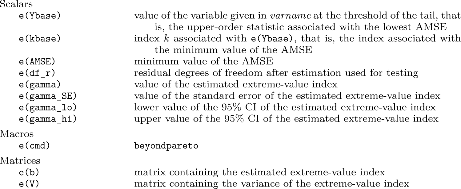
3.3 Stored results

beyondpareto stores the following in e ():

4 The pqqplot command

The Pareto QQ plot can be generated separately using the pqqplot command.

4.1 Syntax

pqqplot runs in Stata 11.2 and later versions. The syntax is

pqqplot varname [ if ][ in ][ weight ], gamma( # ) base( # )

[save ( string ) maxk( # ) size(string) hidden_plots]

The command shows a custom Pareto QQ plot with an assumed $\gamma$ and a chosen threshold upper-order statistic k. Essentially, the requirements are as with beyondpareto: the command requires one variable with numerical data of values greater than zero. Weights are assumed to be survey weights as described in section 2. pweights are allowed; see [U] 11.1.6 weight.

4.2 Options

gamma(#) specifies the assumed extreme-value index used to plot a line for the upper tail of the data. gamma() is required.

base(#) specifies the threshold upper-order statistic beyond which the data are assumed to become linear. The plotted line depending on gamma () also starts only at the specified base. base () is required.

save (string) specifies that the plot be saved under a supplied filename, which needs to be given as newfilename. suffix, where suffix can be chosen from the list of formats given in graph export, along with other options.

maxk(#) specifies up to which upper-order statistic the graph should be plotted.

size (string) specifies the size of the graph. The syntax is identical to [G-3] region_options , and one can set size(xsize(#)), size(ysize(#)), or both via size(xsize(#) ysize(#)).

hidden_plots plots the graph with the nodraw option so that the graph is not visible.

5 Applications

This section provides several applications. The first application is an illustration based on synthetic data capturing the standard empirical challenge that practitioners face when fitting heavy-tailed distributions. The second application uses wealth data from Germany and demonstrates the differences between shape parameters from ad hoc selections of lower thresholds and the optimal threshold. The third example is a replication of Schluter (2021), focusing on city-size distribution in Germany.

5.1 Synthetic data examples

5.1.1 Example 1a:Performance evidence for the lognormal-Pareto model

A popular parametric model for income, wealth, and city-size data consists of assuming that a Pareto upper tail is smoothly pasted on a lognormal body (a so-called lognormal-Pareto [LN-P] model).⁵ See Jenkins (2017) for an example focusing on top incomes, while Vermeulen (2018) considers top wealth and Ioannides and Skouras (2013) consider the city-size distribution.

The data-generating process (DGP) is as follows (the replication code is included in the help file for beyondpareto): We draw a synthetic dataset of 3,000 observations following a lognormal distribution. The mean of the underlying normal variate is 5, and the standard deviation is 2. An additional 2,000 observations populate the upper tail and follow a Pareto distribution; that is, $F(y)=1-(y/Y_{\mathrm{base}}{)}^{-1/\gamma }$ for $y\ge Y_{\mathrm{base}}$ and O otherwise, with $\gamma$  = 1/0.85 = 1.176 and threshold $Y_{\mathrm{base}}=242.51$ . Hence, by construction, the threshold value that marks the beginning of the Pareto tail is known such that the evaluation of the performance of beyondpareto is straightforward.

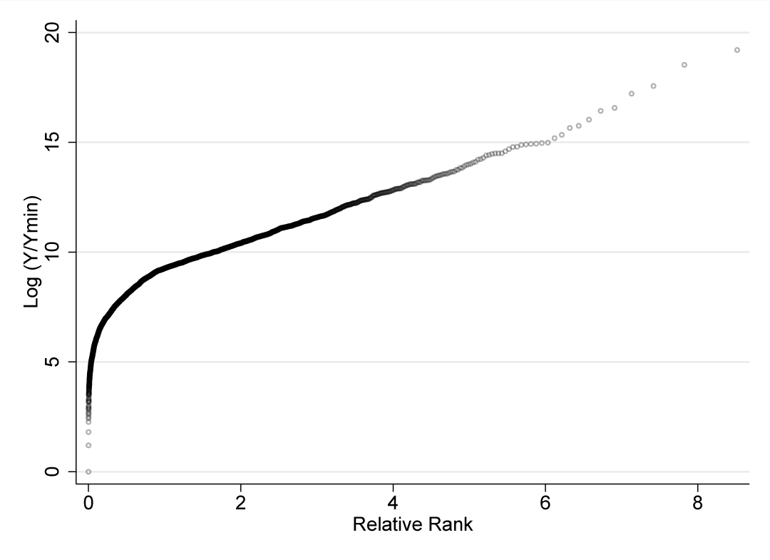
Figure 1 shows the Pareto QQ plot for example 1a. The x axis gives the relative rank of each observation as defined in section 2, while the y axis gives the log of relative income (income relative to minimum y in the dataset). The Pareto QQ plot becomes eventually linear, but it is not immediately apparent from visual inspection at which precise relative rank that is. Executing

beyondpareto y, nrange(10,5000) rho(-0.5) plot(all)

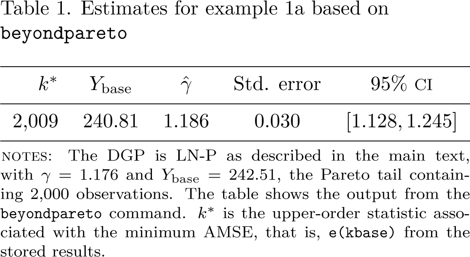
in Stata yields a regression table and a figure with three graphs. Table 1 displays the regression. The selected threshold of $k^{*}=2,009$ is very close to actual threshold value of 2,000. The $95\text{\%}$ CI of the estimated shape parameter [1.128, 1.245] is tight and contains the underlying true value of 1.176.

Figure 1.

Pareto QQ plot for example la

Table 1.

Estimates for example la based on beyondpareto

$k^{*}$	$Y_{\mathrm{base}}$	$\hat{\gamma }$	Std. error	95% CI
2,009	240.81	1.186	0.030	[1:128; 1:245]

NOTES: The DGP is NP as described in the main paper. γ = 1.176 and λ_base = 342.513. The Pareto tail contains 2000 observations. The table shows the output of the pre-optimization command. k* is the upper-order statistic associated with the minimum AMSE, that is, e(kbase) from the pre-optimization results.

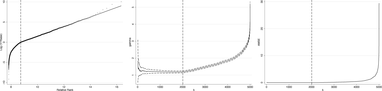
Figure 2 provides the three automatically generated diagnostic plots (Pareto QQ plot, $\gamma$ , and AMSE). The left-hand graph corresponds, up to a constant shift on the y axis to the Pareto QQ plot from figure 1. In addition, the vertical line indicates the optimal threshold, and the slope of the black straight line corresponds to $\hat{\gamma }$ . This plot indicates that $k^{*}$ has been chosen at a point where the Pareto QQ plot just starts to become linear [estimated relative rank equals about 0.912 (true: 0.916)] and that the estimated shape parameter nicely fits the tail. The graph in the middle of the figure shows the variability of the estimates of the shape parameter, $\gamma$ , with respect to threshold values k. For thresholds rather stable, and the optimal value $k^{*}$ lies at the very end of that fat segment of the plot, thus minimizing the variance of the estimator in this range. The right-hand graph gives the AMSE as a function of thresholds, k. It is small and has a long fat segment that slowly starts to rise for thresholds exceeding 2,000. In sum, the three plots are reassuring in that the procedure 1) correctly identifies the lower threshold of the Pareto tail and 2) estimates an extreme-value index that nicely fits this tail.

Figure 2.

Diagnostic plots for example la

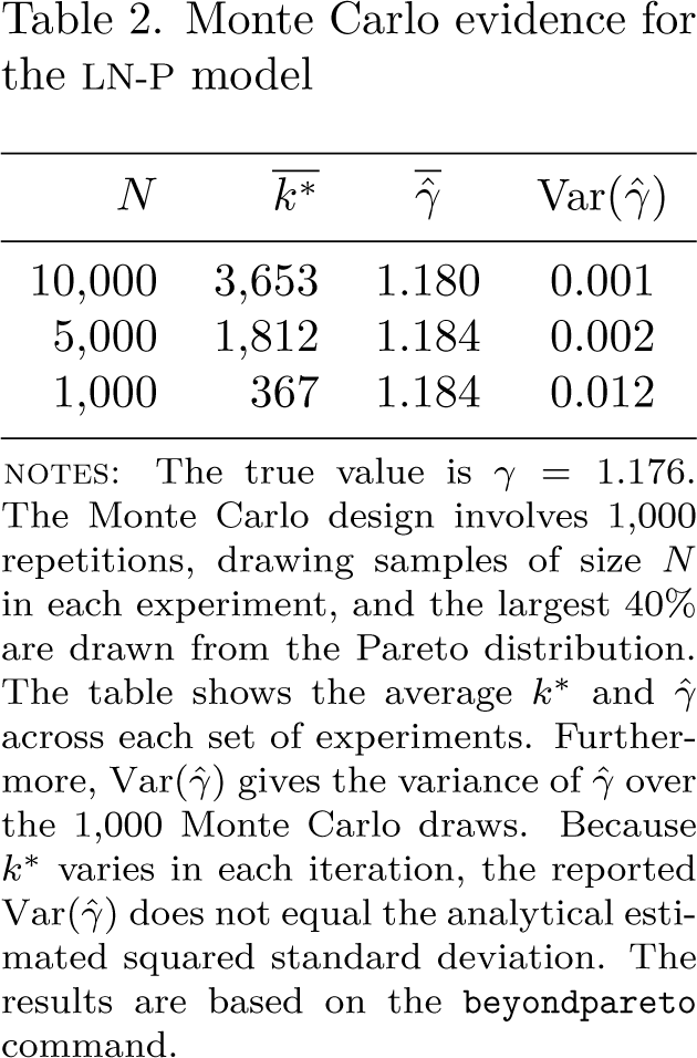
To close the example, we consider whether beyondpareto performs well at over 1.000 Monte Carlo draws of the LN-P DGP and at different sample sizes. In table 2, we show the Monte Carlo average of $k^{*}$ ， $\hat{\gamma }$ , and the variance of $\hat{\gamma }$ over the Monte Carlo draws Throughout, $\gamma$ is well estimated.

Table 2.

Monte Carlo evidence for the LN-P model

N	$\overline{k*}$	$\overline{\hat{\gamma }}$	Var( $\hat{\gamma }$ )
10.000	3.653	1.180	0.001
5.000	1.182	1.184	0.002
1.000	.367	1.184	0.012

NOTES. The true value is $\gamma =1,176$ . The Monte Carlo design involves 1,000 repetitions, drawing samples of size N in each experiment, and the largest 40% are drawn from the Pareto distribution. The table shows the average ${\kappa }^{*}$ and $\hat{\gamma }$ across each set of experiments. Furthermore, Var $(\hat{\gamma })$ gives the variance of $\hat{\gamma }$ over the 1,000 Monte Carlo draws. Because ${\kappa }^{*}$ varies in each iteration, the reported Var $(\hat{\gamma })$ does not equal the analytical estimated squared standard deviation. The results are based on the beyondpareto command.

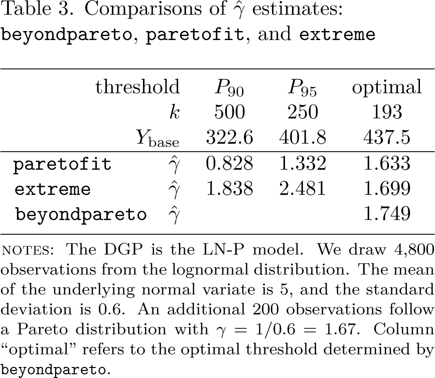
Last, we compare beyondpareto with two existing implementations: paretofit and extreme (see footnote 1). In both cases, the threshold value for inclusion of the upperorder statistics needs to be supplied by the user. Following many applied researchers, we choose the top $10\text{\%}$ or $5\text{\%}$ quantiles as cutoffs. If, for a particular dataset, these cutoff choices exceed beyondpareto’s $k^{*}$ ，then all three functions will usually yield similar point estimates. If not, the resulting extreme-value index estimates are likely to be distorted. Table 3 illustrates this situation for the LN-P setting assuming $\gamma$  = 1.67 beyondpareto’s optimal choice of $k^{*}=193$ , implying $Y_{\mathrm{base}}=437.5$ , yields a $\gamma$ estimate of 1.75. However, the estimates of $\gamma$ by paretofit and extreme are distorted: For $P_{90}$ (implying $Y_{\mathrm{base}}=322.6$ ，the $\gamma$ estimates for paretofit and extreme are 0.828 and 1.838, respectively; for $P_{95}$ (implying $Y_{\mathrm{base}}=401.8$ , these estimates are 1.332 and 2.481. By contrast, using beyondpareto’s optimal choice $k^{*}=193$ , all three methods yield estimates of $\gamma$ close to the population value.

Table 3.

Comparisons of $\tilde{\gamma }$ estimates beyondpareto, paretofit, and extreme

	Threshold	$P_{90}$	$P_{95}$	optimal
	$k$	500	250	193
	$Y_{\mathrm{base}}$	322.6	401.8	437.5
paretofit	$\overline{\gamma }$	0.828	1.332	1.663
extreme	$\overline{\gamma }$	1.838	2.481	1.699
beyond pareto	$\overline{\gamma }$			1.749

NOTES: The DGP is the LN-P model. We draw 4,800 observations from the lognormal distribution. The mean of the underlying normal variate is 5, and the standard deviation is 0.6. An additional 200 observations follow a Pareto distribution with $\gamma =1/0.6=1.67$ . Column “optimal” refers to the optimal threshold determined by beyondpareto.

5.1.2 Example 1b: Performance evidence for the Burr model

Consider next the Burr distribution $1-F_{(\gamma ,\rho )}(y)=(1+y^{-\rho /\gamma }{)}^{1/\rho }$ with $\gamma >0$ and $\rho <0$ (the latter being in fact the second-order parameter of regular variation). In the inequality literature, it is also known as the Singh-Maddala distribution (Singh and Maddala 1976). For large y, the distribution can be expanded as $y^{-1/\gamma }\{1+(1/\rho )y^{\gamma /\rho }\}$ which reveals the Burr distribution to be a member of the Hall class. Its tail quantile is $U(y)=y^{\gamma }\{1+(\gamma /\rho )y^{\rho }+o(y^{\rho })\}$ .

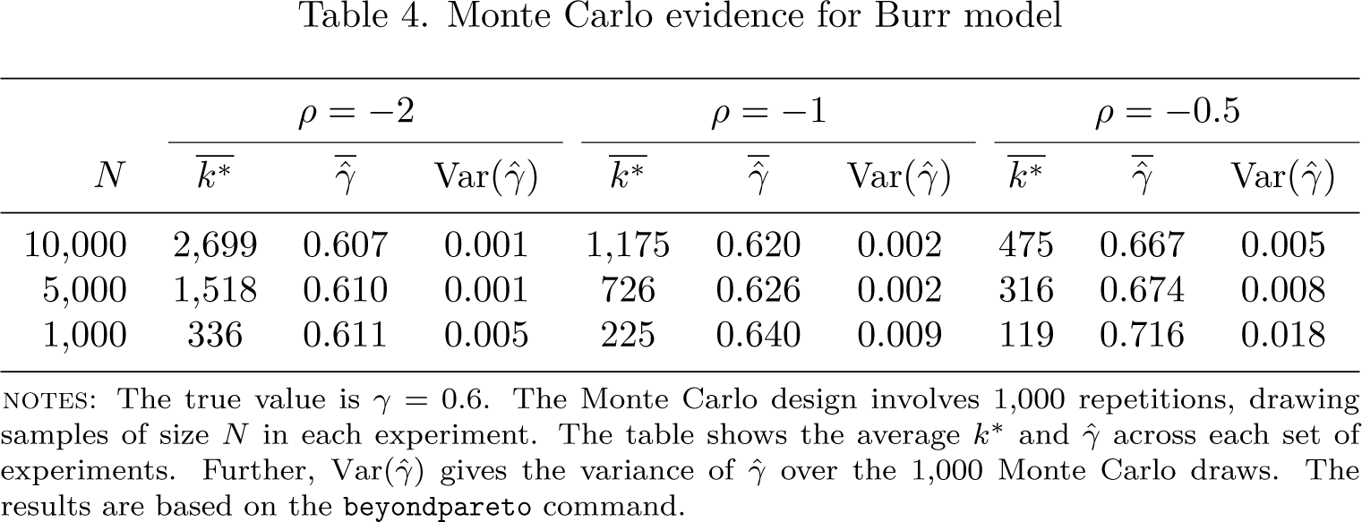
The study of the estimator of $\gamma$ in the Burr case is instructive of the empirical challenges given by a slow convergence to the Pareto limit, parameterized here by $\rho$ . Table 4 presents some Monte Carlo performance evidence for various values of $\rho$ and sample sizes based on beyondpareto. For $\rho =-2$ , the estimator is well behaved even for samples of size 1,000. However, as the magnitude of $\rho$ falls to -0.5 the performance of the estimator deteriorates. Balancing the tradeoff between bias and variance, the AMSE-based choice leads to a sharply decreasing $k^{*}$ .

Table 4.

Monte Carlo evidence for Burr model

	ρ = –2			ρ = –1			ρ = –0.5
$N$	$\overline{k^{*}}$	$\overline{\hat{\gamma }}$	Var( $\hat{\gamma }$ )	$\overline{k^{*}}$	$\overline{\hat{\gamma }}$	Var( $\hat{\gamma }$ )	$k^{*}$	$\overline{\hat{\gamma }}$	Var( $\hat{\gamma }$ )
10,000	2,699	0.607	0.001	1,175	0.620	0.002	475	0.667	0.005
5,000	1,518	0.610	0.001	726	0.626	0.002	316	0.674	0.008
1,000	336	0.611	0.005	225	0.640	0.009	119	0.716	0.018

NOTEs: The true value is $\gamma =0.6$ The Monte Carlo design involves 1.000 repetitions, drawing samples of size N in each experiment. The table shows the average $k^{*}$ and $\hat{\gamma }$ across each set of experiments. Further, $\mathrm{Var}(\hat{\gamma })$ gives the variance of $\hat{\gamma }$ over the 1,000 Monte Carlo draws. The results are based on the beyondpareto command.

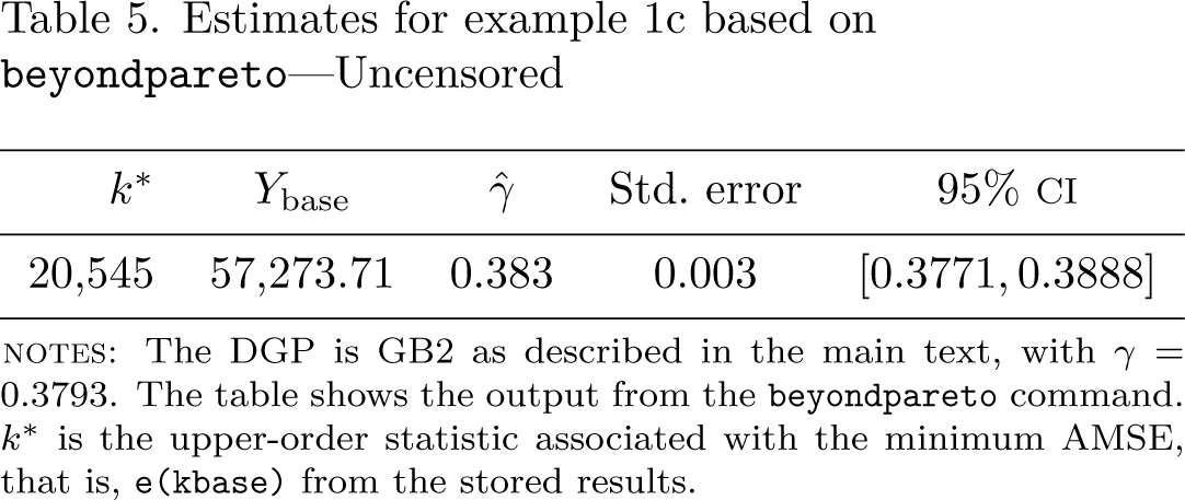
5.1.3 Example 1c: Top-censoring in the GB2 model

Next we illustrate the merit of our weighting procedure in the context of top-censoring Administrative earnings data are often top-coded. For instance, earnings in the well known German Sample of Integrated Labour Market Biographies data are censored at the social security contribution threshold, leading to an average censoring incidence of about $12\text{\%}$ in the earnings distribution of prime-aged male workers in West Germany in recent years. For this population, Schluter and Trede (2024) demonstrate that the heavy-tailed GB2 distribution provides an excellent fit to earnings data at the national level (as well as at the level of cities). The GB2 density has four parameters and is given by $f(x;a,b,p,q)=a{x}^{ap-1}/[b^{ap}B(p,q){\{1+{(x/b)}^a\}}^{p+q}]$ ，where $B(.,.)$ denotes the beta distribution. It is well known that $\gamma =1/(aq)$ . In the following experiment, we use parameter estimates from Schluter and Trede (2024). Specifically, the parameter vector is (5.18,32754,0.518,0.509), implying a population extreme-value index of $\gamma =0.3793$ In the first step, we verify that the estimator performs well in this setting. For a random sample of 140,000 observations, typing

beyondpareto income,fracrange(.0001,.2) rho-0.5

yields the results reported in table 5.

Table 5.

Estimates for example lc based on beyondpareto-Uncensored

k*	Y base	$\hat{\gamma }$	Std. error	95% ci
20,545	57273.71	0.383	0.003	[0.3771, 0.3888]

notes: The dgp is gb2 as described in the main text, with $\gamma =0.3793$ . The table shows the output from the beyondpareto command. $k^{*}$ is the upper-order statistic associated with the minimum amse that is, e(kbase) from the stored results.

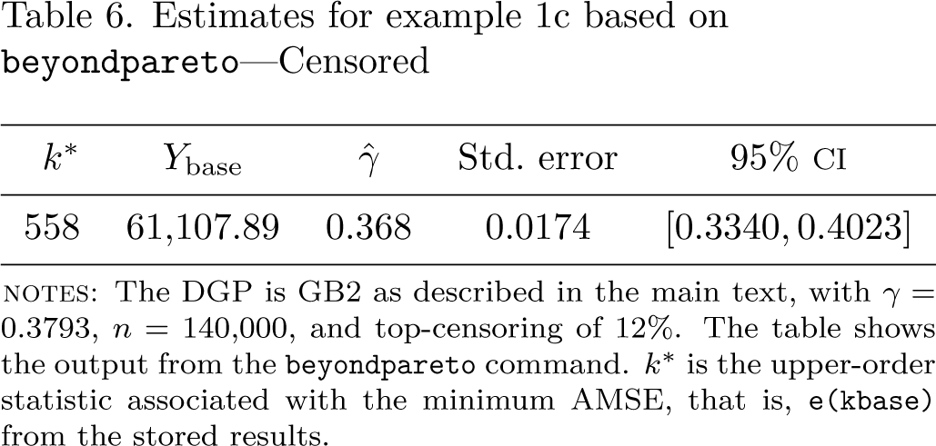
Next we investigate the effect of top-censoring on the estimator, imposing a censoring incidence of $12\text{\%}$ (as in the administrative Sample of Integrated Labour Market Biographies data). Because the distribution now has a mass point at the censoring threshold, we adjust the weight of one such worker by adding the total weight of all censored individuals and drop the remaining censored observations. Executing

beyondpareto income [w = weight],fracrange.003,.2) rho-0.5

yields the results reported in table 6. Despite such a large censoring incidence, the weighted rank-size estimator perforims well. By contrast, if the censoring problem is not properly addressed (by either ignoring it or dropping all censored observations), it can be easily verified that the estimator is then biased.

Table 6.

Estimates for example 1c based on beyondpareto—Censored

k*	Y base	$\hat{\gamma }$	Std. error	95% ci
558	61,107.89	0.368	0.0174	[0.3340, 0.4023]

notes: The DGP is GB2 as described in the main text, with $\gamma =$ 0.3793, $n=140,000$ , and top-censoring of $12\text{\%}$ . The table shows the output from the beyondpareto command. $k^{+}$ is the upper-order statistic associated with the minimum AMSE, that is, e (kbase) from the stored results.

5.2 Example 2: Top wealth in Germany

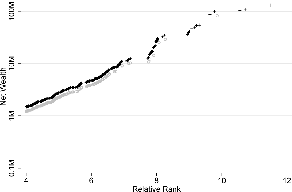
Our next example builds on Konig, Schluter, and Schroder (2023) and uses data from the German Socio-Economic Panel (soep) to examine the top tail of the German wealth distribution in 2019,⁶ when the soep collected household net wealth for its regular samples and for a newly launched top wealth sample (soep-p). soep-p was collected from a sampling frame building on register data on firm ownership in Germany (Schroder et al. 2020). The sample is fully integrated into the panel and is equipped with appropriately constructed survey weights. As detailed in Konig, Schluter, and Schroder (2023), the oversampling of the wealthy, especially of multimillionaires was successful, thus addressing the well-known “missing rich” problem in standard survey data. However, because soep-p did not achieve full coverage in the range of (multi)billionaires, it is appropriate to construct inequality statistics based on a (parametric)model of the upper tail of the wealth distribution. See Konig, Schluter, and Schroder (2023) for full details of the procedure and performance evidence.

Figure 3 provides the Pareto QQ plot of (nonnormalized) household net wealth, with 十 signs indicating observations from the soep-p sample, where we have zoomed into the upper tail for better visual clarity. soep-p clearly clusters in the upper tail of the distribution and thickens the upper tail of the net wealth distribution as observed in the SOEP. Apart from infilling, the SOEP-P sample also appends an upper tail.

Figure 3.

Pareto QQ plot for SOEP wealth data

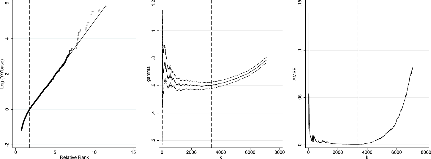
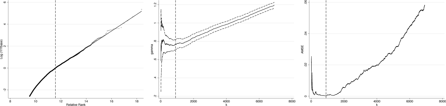
Because the soep has a complex survey design, sample weights can and should be used (thus the function call extends example 1 above). Let weight denote SOEP household weights and wealth household net wealth. Executing

beyondpareto wealth [w = weight],fracrange.00071813,0.51) rho-0.5 plot(all)

in Stata produces table 7 and figure 4. Similarly to the synthetic data example, the Pareto QQ plot becomes linear eventually, but the precise location is not immediately obvious.

Figure 4.

Diagnostic plots for example 2

Table 7.

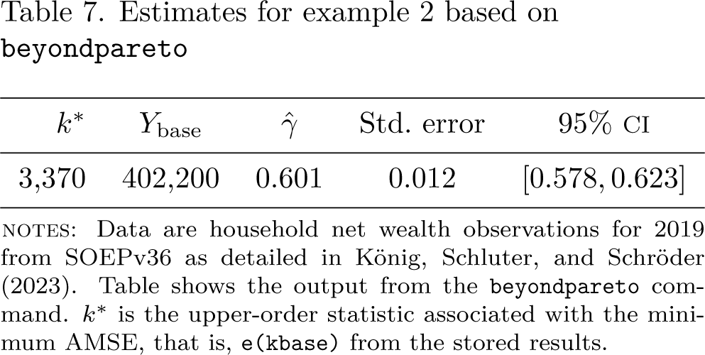
Estimates for example 2 based on beyondpareto

Y base	Y base	$\hat{\gamma }$	Std. error	95% ci
3,370	402,200	0.601	0.012	[0:578; 0:623]

notes: Data are household net wealth observations for 2019 from SOEPv36 as detailed in König, Schluter, and Schröder (2023). Table shows the output from the beyondpareto command. $k^{*}$ is the upper-order statistic associated with the minimum AMSE, that is, e(kbase) from the stored results.

At slightly more than 400,000 euros, the optimal threshold is lower than usual practitioners’ ad hoc threshold choices (one or two million euros in the German context; see Vermeulen [2018], Bach, Thiemann, and Zucco [2019]). The associated Pareto coefficient is a tightly estimated 1/0.601 = 1.664 $95\text{\%}$ ci [1.605,1.730]), indicating that wealth concentration in Germany is high. The Pareto QQ plot indicates that the Pareto distribution is a reasonable approximation of household net wealth in Germany. The $\gamma$ and amse plots show that the selected thresholds imply an estimate of $\gamma$ from a stable and fat region. Pareto coefficients for practitioner thresholds of one and two million euros are 1.671 (95% Cl: [1.576, 1.779]) and 1.518 ( $95\text{\%}$ ci: [1.396, 1.664]), respectively, which suggests for one million slightly lower and for two million slightly higher wealth concentration. Note, however, that the confidence bands are somewhat wider.

5.3 Example 3: The German city-size distribution

The last example replicates the results reported in Schluter (2021), and the full replication code is included in the help file for beyondpareto. We consider the size distribution of cities in Germany in 2000, using administrative data provided by the German Federal Statistical Office. These administrative data are highly accurate because of the legal obligation of citizens to register with the authorities. The unit of analysis is the “city” or, more precisely, the municipality or settlement (“Gemeinden”).

Downloading the data as detailed in beyondpareto’s help file and calling the function

beyondpareto citysize, fracrange(0.001,0.5) rho(-0.5) plot(all)

as before, yields the results reported in table 8 and the plots of figure 5. The optimal threshold is $k^{*}=903$ , which seems a very sensible choice because the plot of $\hat{\gamma }(k)$ in the interval $[350,k^{*}]$ appears fairly fat, so the best choice in this interval is then the largest one to minimize the variance. The estimate of the extreme-value index is $\hat{\gamma }=0.762$ and the precision of the estimate permits a sound rejection of Zipf’s “law”, that is, the hypothesis that $\gamma$ be unity.

Figure 5.

Diagnostic plots for example 3

Table 8.

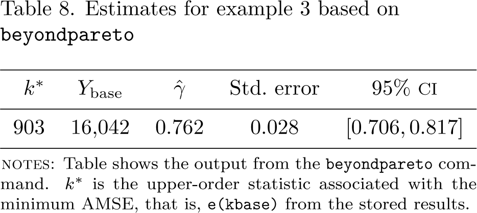
Estimates for example 3 based on beyondpareto

Y base	Y base	$\hat{\gamma }$	Std. error	95% ci
903	16,042	0.762	0.028	[0.706, 0.817]

notes: Table shows the output from the beyondpareto command. $k^{*}$ is the upper-order statistic associated with the minimum amse, that is, e(kbase) from the stored results.

Finally, it is also of substantive interest to observe that the tail index of the city size distribution is very stable. When we adjust the online data access path as detailed in beyondpareto’s help file, the analysis is easily repeated for other years. In particular, we obtain for the year 2010 $\hat{\gamma }(k)=0.77$ with optimal threshold value $k^{*}=1,336$ and for the year 2020 $\hat{\gamma }(k)=0.76$ with optimal threshold value $k^{*}=1,220$ .

6 Conclusion

The core functionality of beyondpareto is the (fast, Mata-coded) estimation of the extreme-value index for heavy-tailed distributions, allowing for complex survey design. Interest in the behavior of size distributions spans many fields, and we have provided applications to wealth, earnings, and city-size distributions. All of these examples are Pareto-like, so the associated Pareto QQ plot becomes linear only eventually, rendering the estimation of its slope parameter using existing software implementations and ad hoc threshold selection problematic. Our choice of the threshold parameter for data inclusion in the tail index estimation is optimal in the AMSE sense; we provide several diagnostic plots for transparency so that the user can critically examine goodness of fit and sensitivities. The workfow is automatized for ease of use. Based on this core functionality, beyondpareto is evolving, including the computation of wealth shares at the top (as in Konig, Schluter, and Schroder [2023] using the newly launched top wealth sample of the SOEP) and imputation methods for top-censored administrative earnings data (see Beckmannshagen et al. [2024] for an application on the record-linked SOEP-RV data).

7 Acknowledgments

Johannes König, Christian Schluter, and Carsten Schröder gratefully acknowledge financial support from the Deutsche Forschungsgemeinschaft (dfg) and the Agence Nationale de la Recherche (anr) for funding the project “Life-Cycle Inequality Dynamics(grant anr-19-fral-0006-01). Johannes Konig and Carsten Schröder gratefully acknowledge financial support by Deutsche Forschungsgemeinschaft (project “Wealth holders at the Top” [watt], project number: 430972113). Isabella Retter gratefully acknowledges funding by dtec.bw— Digitalization and Technology Research Center of the Bundeswehr (project Socio-Economic Panel Linked Employer-Employee Data Version 2 [soep-lee2]).

8 Programs and supplemental material

To install the software files as they existed at the time of publication of this article type

. net sj25-1

. net install st0770 (to install program files, if available)

. net get st0770 (to install ancillary files, if available)

Supplemental Material

sj-txt-1-stj-10.1177_1536867X251322969 - Supplemental material for The beyondpareto command for optimal extreme-value index estimation

Supplemental material, sj-txt-1-stj-10.1177_1536867X251322969 for The beyondpareto command for optimal extreme-value index estimation by Johannes König, Christian Schluter, Carsten Schröder, Isabella Retter, and Mattis Beckmannshagen in The Stata Journal