miesize: Effect-size calculation in imputed data

Abstract

In this article, I describe the miesize command for the calculation of effect sizes in imputed data. There may be situations where an effect size needs to be estimated for an intervention, an exposure, or a group membership variable but data on the independent or dependent variable are missing. Such missing data are commonly dealt with by multiply imputing plausible values. However, in this circumstance, the estimated effect size and associated standard errors will need to be pooled and estimated from the imputed dataset. The miesize command automates this process and calculates effect sizes for a binary variable from multiply imputed data in wide format. The estimates and standard errors (used to calculate the confidence intervals) are recombined using Rubin’s (1987, Multiple Imputation for Nonresponse in Surveys [Wiley]) rules. These rules are applied such that the average point estimate for the effect size is calculated from the imputed datasets. The pooled standard error, and hence confidence intervals, is calculated to account for both the variance between the imputed datasets and the variance within them. Pooled effect sizes and confidence intervals for Cohen’s (1988, Statistical Power Analysis for the Behavioral Sciences, 2nd ed. [Lawrence Erlbaum]) d, Hedges’s (1981, Journal of Educational Statistics 6: 107-128) g, and Glass’s (Smith and Glass, 1977, American Psychologist 32: 752-760) delta are provided by miesize.

1 Introduction

The term “effect size” usually refers to the magnitude, and direction, of an association between two variables or the mean difference between two groups. Statistical tests that produce p-values indicate the probability that the observed result, or one more extreme, was due to chance alone. In contrast, effect sizes indicate the magnitude of the association between variables, or mean group difference. Such estimation is intended to help interpret the results and understand what they may mean in practical terms. For example, in a healthcare situation, an experimental treatment may result in a statistically significant difference in a symptom outcome between the experimental and control group. However, the treatment is unlikely to be useful in practice unless the magnitude of the difference is clinically meaningful—that is, one that makes a difference to the average quality of life of patients.

In relation to estimating a mean difference for a continuous outcome across groups, these methods are sometimes referred to as the “d” family. The average group difference described by an effect size could be applied to experimental data. In this situation, the mean value of an outcome of interest between a group of individuals randomized to either an experimental intervention or a control condition is compared and contrasted. In observational data, the mean value can refer to a mean intergroup difference in relation to a sociodemographic or other characteristic.

Effect sizes, relating to a mean group difference, can be described in the original metric of an outcome measure. However, these may not be easily interpretable. For example, the outcome may relate to an attitudinal questionnaire, with responses scored and summed according to a Likert scale. Some experts may understand what a difference of “five points” may mean in this situation, but many others would not. Thus, the term “effect size” often refers to such differences quantified in a standardized metric. The d family of estimators provides an effect size that is standardized according to the standard deviation (sd) (that is, square root of the variance) of the outcome of interest. All the d family of estimators assume that the outcome of interest is normally distributed, and thus, departure from this can introduce bias (Grissom and Kim 2001).

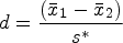
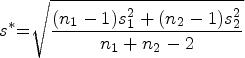
One of the most commonly used metrics of effect size is Cohen’s (1988) d. For Cohen’s d, standardization is performed according to the pooled SD for both groups being compared (see below). In general, the d family communicates effect size as the scaled difference between the means, divided by the SD of the outcome of interest. Here we see in the following equation that Cohen’s d is given by the difference in the means of the outcome between the two groups ( ${\overline{x}}_1$ and ${\overline{x}}_2$ ) divided by the pooled SD (s*):

$$d={\displaystyle \frac{({\overline{x}}_1-{\overline{x}}_2)}{s^{*}}}$$

The pooled SD (S*) is calculated as

$$s^{*}=\sqrt{{\displaystyle \frac{(n_1-1)s_1^2+(n_2-1)s_2^2}{n_1+n_2-2}}}$$

where $n_1$ and $n_2$ refer to the number of observations in each of the two comparison groups, respectively. Here $s_1$ and $s_2$ are the SDs of the outcome for each respective group.

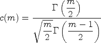
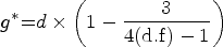
However, Hedges showed that Cohen’s d can be biased, especially when there are relatively small numbers of observations (for example, N < 20), and proposed a correction factor could be applied to d (Hedges 1981; Hedges and Olkin 1985). Let d represent Cohen’s d and m the summed total number of observations across groups (that is, $m=n_1+n_2$ ). Where Γ represents the gamma function, Hedges’s g is calculated as $g=d\times c(m)$ , where

$$c(m)={\displaystyle \frac{\mathrm{\Gamma }\left({\displaystyle \frac{m}{2}}\right)}{\sqrt{{\displaystyle \frac{m}{2}}}\mathrm{\Gamma }\left({\displaystyle \frac{m-1}{2}}\right)}}$$

Though not implemented in Stata, Hedges also provided a simplified version of the correction factor. This is slightly biased but computationally easier to calculate. Here d.f. represents the degrees of freedom, given by d.f. $=n_1+n_2-2$ , for an independent group design (Borenstein et al. 2021). Once again, d represents Cohen’s d, and this approximation (g*) is calculated as

$$g^{*}=d\times \left(1-{\displaystyle \frac{3}{4(\mathrm{d}.\mathrm{f})-1}}\right)$$

Both Cohen’s d and Hedges’s g use the pooled variance of the outcome. In contrast Glass’s delta (Δ) provides two effect sizes, Δ₁ and Δ₂, relating to the variance in the respective groups of observations. Where ${\overline{x}}_1$ and ${\overline{x}}_2$ once again represent the group means of the continuous outcome, and s₁and s₂ represent the group specific SDs for the outcome, Glass’s Δs are calculated as

$$\begin{array}{rl}& {\mathrm{\Delta }}_1={\displaystyle \frac{{\overline{x}}_1-{\overline{x}}_2}{s_1}}\\ & {\mathrm{\Delta }}_2={\displaystyle \frac{{\overline{x}}_1-{\overline{x}}_2}{s_2}}\end{array}$$

Originally, this approach was intended to be applied to experimental data where Δ₁ related to the control group (Smith and Glass 1977). For experimental data, usually the SD for the control group is used when calculating Δ. However, for observational data, the choice of which of the group’s SD to use appears arbitrary, while for dummy- coded group variables (one or zero/absent or present), the group with “zero” status could be the one to have the SD used in calculating Δ. However, in the absence of a compelling reason to consistently report Δ based on one or the other group’s SD, it has been recommended that both effect-size estimates (Δs) be reported for observational data (Kline 2013).

Irrespective of the method used, there are well-known rules of thumb for interpreting effect sizes. That is, effect sizes of 0.2 to 0.5 are usually regarded as “small/modest”, 0.5 to 0.8 as “medium sized”, and 0.8 or above as “large sized”. However, these interpretations will need to be contextualized. For example, in healthcare it is for stakeholders and experts (patients and clinicians) to agree on what magnitude of difference may be considered to constitute a clinically meaningful effect size. Moreover, from an economic perspective, cost effectiveness of an intervention may not be achieved even with an effect size that is classed as “large” in this context. Thus, it is important to understand the meaning and implications of an effect size within its specific substantive context.

Missing data may be present in both experimental design and observational studies. Analyzing data using listwise deletion may give biased results. It is also wasteful of the information available in the remaining values in the variables that are present in observations with one or more missing values. Thus, best practice when analyzing data with missing values is to use multiple imputation (van Ginkel et al. 2020; Sterne et al. 2009). This involves drawing plausible values for those missing from conditional probability distributions. These distributions are shaped by the relationship observed between the variables for which the values are nonmissing. These values are imputed for multiple datasets (usually five or more), and the results recombined. Such results are unbiased if the data are missing completely at random (that is, because of chance only) or missing at random (missing values depend on the observed values of variables) according to Rubin’s (1987) missing data mechanism classification. Indeed, even if the data are not missing at random (the missing values may depend on unobserved variable values), the results from multiply imputed data may be less biased than that derived from listwise deletion (van Ginkel et al. 2020). When recombining the results from multiply imputed data, one must account for the uncertainty introduced by the imputation process when deriving standard errors (SEs). Stata currently offers a wide range of analyses that work with multiply imputed data. These are invoked by using the command after the prefix mi estimate, for example, mi estimate: regress ….

Rubin (1987) provided rules for how means and SEs (and hence confidence intervals) could be combined from results derived from multiply imputed datasets. Known aptly enough as “Rubin’s rules”, these are as follows.

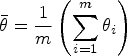
To pool an effect estimate, such as the pooled mean difference $(\overline{\theta })$ , one uses the following formula. Here, on this occasion, m represents the number of imputed datasets used, and i denotes the ith dataset:

$$\overline{\theta }={\displaystyle \frac{1}{m}\left(\sum _{i=1}^m{\theta }_i\right)}$$

This is effectively the mean of the mean differences calculated across the m imputed datasets.

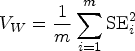
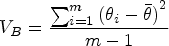
Pooling the SE for such estimates is more complicated and must account for the sampling variance both within and between the imputed datasets. The “within imputation variance” is the average of the mean of the within variance estimate. In effect, this is the squared SE calculated for each imputed dataset. This value reflects the sampling variance in each of the datasets generated by the multiple imputation process. Thus, as expected, this value will be relatively large in small samples and more modest in larger samples (Heymans and Eekhout 2019). It is given by the following equation, where V_W is the within imputation variance:

$$V_W={\displaystyle \frac{1}{m}\sum _{i=1}^m{\mathrm{SE}}_i^2}$$

The between imputation variance is intended to reflect the additional variance due to the uncertainty relating to the value of the imputed data. This is estimated by calculating the variance of the parameter of interest estimated over all the imputed datasets. This formula is the same as that ordinarily used to calculate the variance in a given sample. The value is large when the missing data are extensive and relatively smaller with fewer missing data. Here V_B is the between imputation variance, $\overline{\theta }$ is the overall pooled estimate for the parameter of interest, and ${\theta }_i$ is the parameter of interest estimated in each of the m imputed datasets:

$$V_B={\displaystyle \frac{{\sum }_{i=1}^m{({\theta }_i-\overline{\theta })}^2}{m-1}}$$

To date, Stata does not include a command to estimate effect sizes from multiply imputed data. This function may be useful given that missing data are regularly encountered in experimental and observational data where it may be desirable to calculate effect sizes.

2 The miesize command

2.1 Syntax

miesize varname [ if ] [ in ], by(groupvar) [ glass countdown level(#) ]

varname is the outcome variable of interest. groupvar is a variable that defines the two groups that miesize will use to estimate the effect sizes.

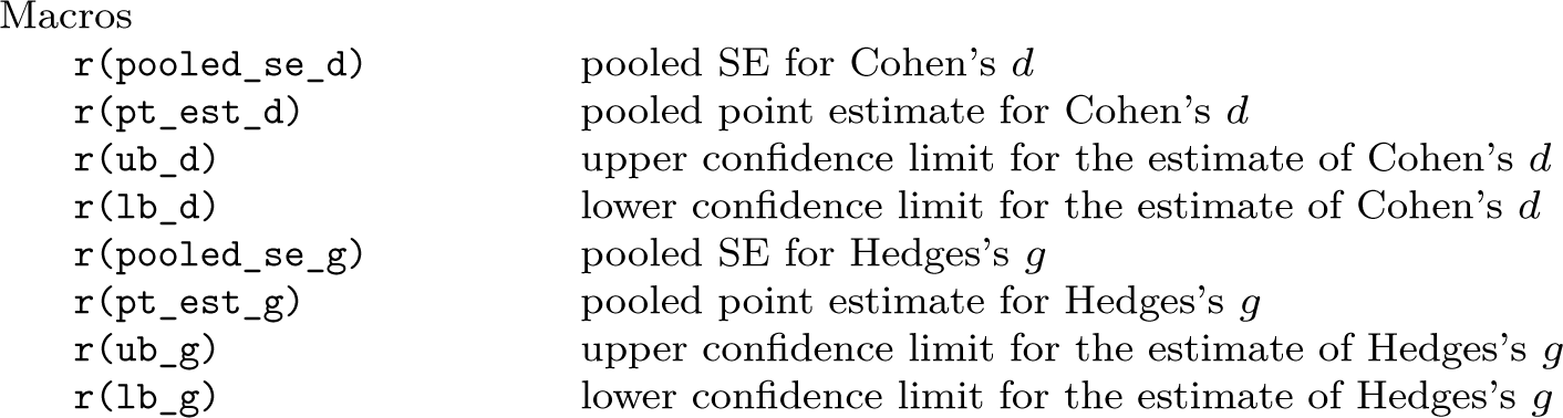
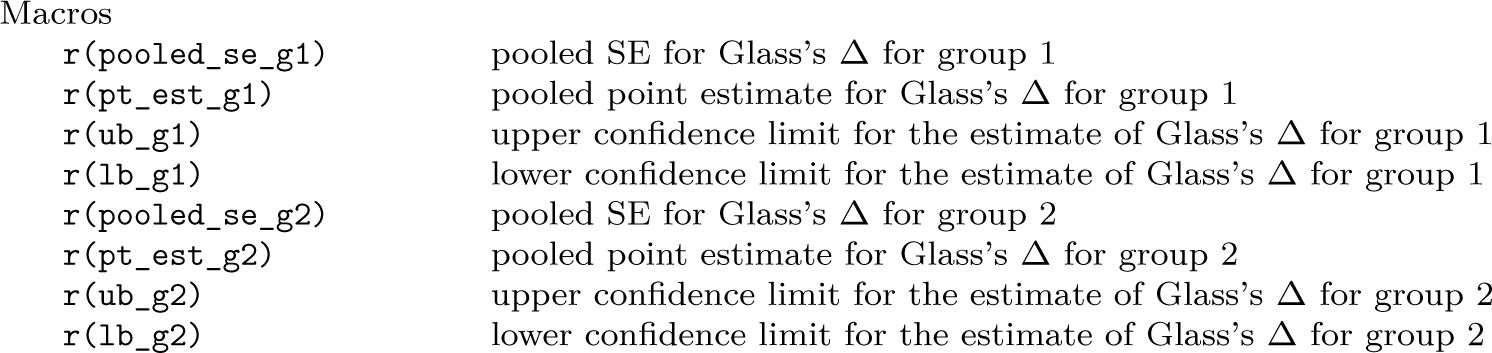
The command returns a range of results in r(). Do not confuse the by() option with the by prefix; you can specify only the former in miesize.

2.2 Options

by(groupvar) specifies the groupvar that defines the two groups that miesize will use to estimate the effect sizes. by() is required.

glass reports Glass’s Δ (Smith and Glass 1977) using each group’s SD.

countdown specifies that a countdown of analysis steps remaining be displayed.

level(#) specifies the confidence level to be reported. This can be set between 10 and 99.99%. The default is level(95).

2.3 Stored results

miesize stores the following results in r():

If the glass option is not specified:

If the glass option is specified:

All methods:

2.4 How to use miesize

The miesize command calculates two-sample effect sizes from multiply imputed data in wide format. The command can handle situations where either one or both variables (namely, the outcome and grouping variables) are imputed. When neither variable is detected as imputed, then the esize command for nonimputed data will be invoked, and a message will be provided to alert the user of this: It appears that neither of the variables is imputed. The standard ‘esize twosample’ analysis will be performed. You may wish to check your imputed data are in standard Stata wide format. The imputed data should be in the wide format that Stata provides. That is, imputed variables are named sequentially as _m_varname, where m is the imputation number, for example, _2_price, where this is the second imputed dataset for the variable price. As described in section 1, Rubin’s rules are used to estimate the pooled effect size, SEs, and hence the associated confidence intervals around the point estimate. The miesize command also operates where only a single imputed value is used for the grouping or outcome variable. miesize also handles the situation where either only the outcome variable contains imputed values or only the grouping variable includes imputed values.

The default for miesize is to calculate Cohen’s d and Hedges’s g. The two methods differ in how they estimate the pooled SD of the two groups, as outlined above. In effect, Cohen’s d uses the arithmetic mean of the two group variances. In contrast Hedges’s g uses a weighted average that accounts for the sample sizes of each group. As mentioned in section 1, Glass’s Δ is more appropriate where the variance of the outcome varies significantly between the two groups. In Stata, this can be formally tested using the sdtest command. In this context, the variance across the groups will be compared. Thus, the form of the command used will be

sdtest varname, by(groupvar)

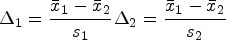
where the varname is the outcome of interest and the groupvar is the group-identifying variable. Where a statistically significant difference between the variances for each group is present, it is likely to be more appropriate to use Glass’s Δ to report the effect size, rather than d or g. For Glass’s Δ, the two effect sizes (Δ₁ and Δ₂) are given relating to the SDs of the two groups. For experimental data, usually the SD for the control group is used when calculating Δ₁. However, as stated earlier, for observational data, the choice of which of the group’s SDs to use appears arbitrary. For dummy-coded group variables (one or zero/absent or present), the group with “zero” status could be the one to have the SD used in calculating Δ₁. However, in the absence of a compelling reason to consistently report a Δ value based on one or the other group’s SD, it has been recommended that both effect-size estimates (Δs) be reported for observational data (Kline 2013).

3 Example

For this example, an analysis of data used for evaluating the recruitment and selection process into UK-based general practice postgraduate medical training is used for illustrative purposes (Tiffin et al. 2024). ¹ One aim of the analysis was to estimate effect sizes in relation to selection test scores for various demographic characteristics. Clearly, any substantial association with such personal qualities would influence the demographics of the population of doctors in training finally selected. In this context, there were complete data for the first stage of selection, which comprised a situational judgment test (SJT) and clinical knowledge assessment (the clinical problem solving [CPS] test). These scores are combined into a summed total that is used in the selection process. While all candidates had SJT and CPS scores, not all had received a standardized face-to-face selection center (SC) assessment. This was a special case of missing data by design. For some years, those who achieved only low combined scores on the SJT and CPS did not proceed to the SC stage. In addition, for some later years, candidates who had achieved relatively high combined SJT and CPS scores were exempted the face-to-face selection stage. Moreover, the face-to-face selection process was suspended completely during the COVID-19 pandemic. Overall, this means that SC scores were not present for around half the doctors in the sample with first-stage selection assessment scores. Thus, estimating the “true” underlying effect size for each demographic characteristic in relation to the scores for the face-to-face SCs required data imputation. This was performed in Stata using chained equations (Royston and White 2011). The estimates from the imputations stabilized after m = 5 imputations, but as a precaution, m = 10 imputed datasets were used. For this particular illustrative example, we will estimate the effect size of male gender on SC scores. Using the sdtest command in Stata, we see the results indicate that the assumption of equal variance in SC scores across gender groups can be rejected:

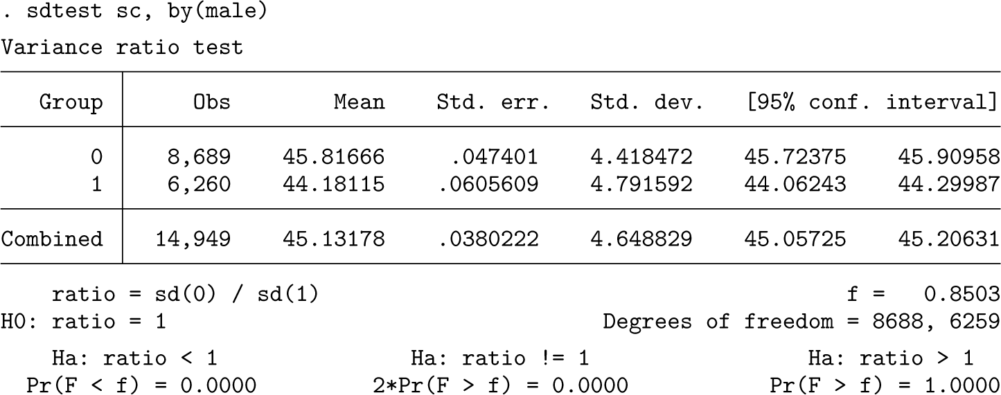
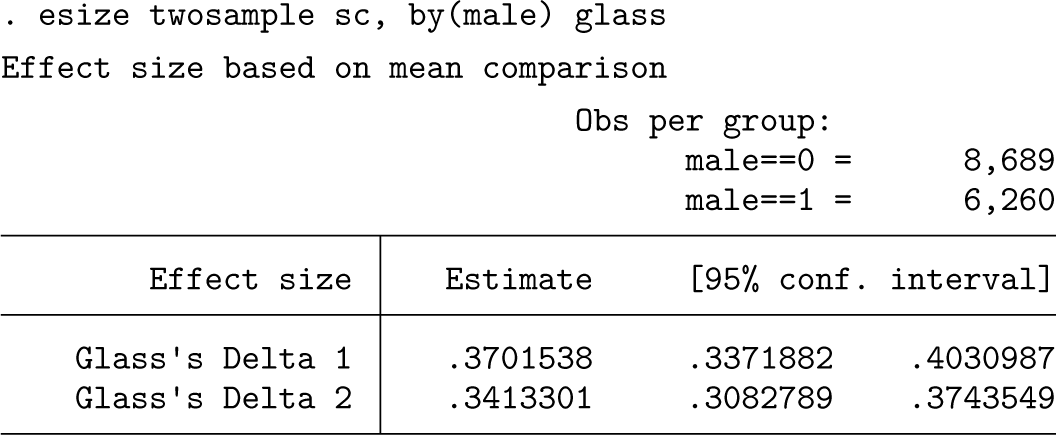
Because there is evidence of unequal variances between the groups, we will use Glass’s Δ to estimate the effect size using miesize:

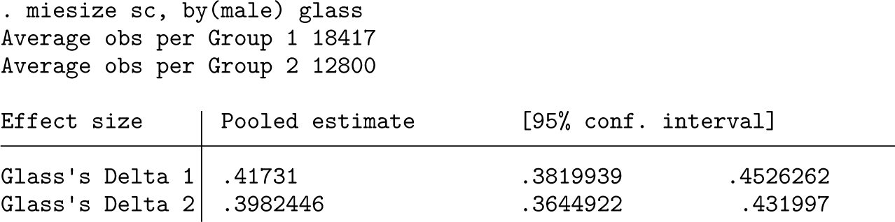
As can be seen from the results, the effect size for male gender is around 0.40 (that is, commonly interpreted as “modest”). As expected, it varies slightly depending on whether the SD of the SC scores for males (0.40) or females (0.42) is used. We can compare our results with those obtained using the esize twosample command, which uses only the observed data:

As might be anticipated, the effect sizes for gender are modestly smaller than those estimated from the imputed data. This is because certain candidates that scored either especially high or low on the first stage of selection tests will not have observable SC scores. Given that, in this sample, males, on average, achieve lower scores on the first- stage assessments, this will produce “indirect range restriction”. This in turn restricts the range of observable SC scores, especially for females. This effect attenuates the effect size observed, a well-recognized phenomenon in personnel selection studies. Indeed, multiple imputation has been shown to be one way of addressing this (Zimmermann, Klusmann, and Hampe 2017; Mwandigha 2017). Thus, the imputed values will offset this effect by simulating the unobserved SC scores. Note that, as expected, the confidence intervals for these effect sizes are slightly wider for the results derived by miesize, compared with esize. This is because, as explained above, the variance between, as well as within, imputed datasets is accounted for. In this case, the former effect is not large. This is because, across the 10 imputed datasets, the imputed SC scores vary little. Indeed, the range of observed SC scores in this sample is 20 to 52. However, between the m = 10 imputed datasets, the imputed SC scores only vary by a range of around 2 points. This is because the relationships between the SC scores and the other variables in the sample are relatively strong. For example, the β coefficient for the SC scores regressed on SJT scores in the observed data is 0.30. Thus, the chained equations impute values with a reasonable level of (apparent) certainty. However, as explained earlier, where the variance in imputed values is higher, this effect will be more marked.

4 Conclusions

The d family of effect size estimators calculates standardized mean group differences for continuous variables. The miesize command avoids the tedious task of calculating the pooled estimates and SEs for these estimators when working with multiply imputed data. A number of limitations with the current miesize command should be acknowledged. At present, neither miesize nor esize accommodates weights (for example, survey weights). Also, the derivation of SEs for both commands rests on an assumption of normality. One way of addressing this would be the option to derive the SEs via bootstrapping, or other resampling methods, which is not presently included for the commands. Note that the standard Stata command esize can be used to calculate effect sizes from unpaired data. This is achieved by calling esize unpaired, then by specifying the two variables of interest with a pair of equal signs between them, for example, esize unpaired mpgl == mpg2. This manner of estimating effect sizes in unpaired data does not currently accommodate multiply imputed data in Stata. Thus, these three limitations offer potential areas for future development of these commands.

Supplemental Material

Supplemental material

Supplemental material