Sage Journals: Discover world-class research

Abstract

Inverse probability of treatment weighting is a popular propensity score-based approach to estimate marginal treatment effects in observational studies at risk of confounding bias. A major issue when estimating the propensity score is the presence of partially observed covariates. Multiple imputation is a natural approach to handle missing data on covariates: covariates are imputed and a propensity score analysis is performed in each imputed dataset to estimate the treatment effect. The treatment effect estimates from each imputed dataset are then combined to obtain an overall estimate. We call this method MIte. However, an alternative approach has been proposed, in which the propensity scores are combined across the imputed datasets (MIps). Therefore, there are remaining uncertainties about how to implement multiple imputation for propensity score analysis: (a) should we apply Rubin’s rules to the inverse probability of treatment weighting treatment effect estimates or to the propensity score estimates themselves? (b) does the outcome have to be included in the imputation model? (c) how should we estimate the variance of the inverse probability of treatment weighting estimator after multiple imputation? We studied the consistency and balancing properties of the MIte and MIps estimators and performed a simulation study to empirically assess their performance for the analysis of a binary outcome. We also compared the performance of these methods to complete case analysis and the missingness pattern approach, which uses a different propensity score model for each pattern of missingness, and a third multiple imputation approach in which the propensity score parameters are combined rather than the propensity scores themselves (MIpar). Under a missing at random mechanism, complete case and missingness pattern analyses were biased in most cases for estimating the marginal treatment effect, whereas multiple imputation approaches were approximately unbiased as long as the outcome was included in the imputation model. Only MIte was unbiased in all the studied scenarios and Rubin’s rules provided good variance estimates for MIte. The propensity score estimated in the MIte approach showed good balancing properties. In conclusion, when using multiple imputation in the inverse probability of treatment weighting context, MIte with the outcome included in the imputation model is the preferred approach.

Keywords

Missing covariates chained equations Rubin’s rules inverse probability of treatment weighting missingness pattern

1 Introduction

Data from observational studies provide useful information to address health-related questions and notably estimate treatment effects in real settings.¹ However, because individuals are not randomised, the treatment groups are often not comparable, which may lead to confounding bias² if these studies are analysed without appropriate adjustment for confounding. Propensity scores (PS) have been proposed as a means to recover balance between groups on observed covariates and so obtain a consistent estimate of the causal treatment effect.³ The PS is defined as the individual’s probability of receiving the treatment rather than the control given their baseline characteristics.⁴ One popular method to achieve covariate balance between treatment groups is to weight individuals by the inverse of their PS. This approach, known as inverse probability of treatment weighting (IPTW),⁵ aims to emulate the sample that would have been observed in a randomised trial.

In practice, a major issue when estimating the PS is the presence of partially observed covariates, as the PS cannot be estimated for individuals with at least one missing covariate value. Standard analyses include complete case analysis⁶ or the missingness pattern approach,⁷ but a popular alternative to handle missing data is multiple imputation (MI).⁸ However, there remain four important unresolved questions about how to implement MI for PS analysis.

First, two approaches to combine information from the imputed datasets have been proposed in the context of PS analyses: combining the treatment effects estimated on each imputed dataset (method called MIte hereafter) or combining for each individual their PS value across the imputed datasets (method called MIps hereafter).^9,10 MIte intuitively seems to adhere best to the MI philosophy by applying the full analysis strategy on each imputed dataset. Furthermore, Seaman and White¹¹ proved that for an infinite number of imputations, the MIte estimator is consistent. However, Mitra and Reiter⁹ published recommendations on the use of MI for PS analysis, and they advocated using MIps, rather than MIte, for PS matching.

The second question is whether or not to include the outcome in the imputation model for the missing covariates. Mitra and Reiter did not include it in their study,⁹ which could explain the bias they observed for both MIte and MIps. One of the advantages claimed for the PS approach in general is that it allows the investigator to use the data on the treatment and covariates to develop a well-fitting PS model without needing to look at the data on the outcome.⁹ This makes it possible to avoid the temptation to search for a PS model that gives a significant treatment effect estimate, a temptation which may be experienced by an analysis which handles confounding by using regression adjustment. Intuition may therefore lead one to believe that imputation of missing covariates should also be done without using the outcome variable.⁹ However, this intuition conflicts with advice to include the outcome when imputing missing covariates in a regression model whose parameters are the quantities of interest.¹²

The third question is how to estimate the variance of the IPTW estimator after MI. When pooling the treatment effects (MIte), Seaman and White¹¹ showed that Rubin’s rule for estimating the variance performs well in practice, although theoretical justification for Rubin’s rules relies on the parameter of interest being estimated with maximum likelihood, which is not the case for the IPTW method. For MIps, there is, to our knowledge, no variance estimator that takes into account both the uncertainty due to the estimation of the PS given the complete data and that due to the imputation of the missing data.

Finally, the fourth question is how well MI performs in comparison to other popular approaches to handle missing data, namely complete case (CC) analysis or the missingness pattern (MP) approach. Qu and Lipkovitch¹³ and Seaman and White¹¹ assessed the performance of MIte additionally including the missingness pattern indicator in the PS model, but they did not compare this approach to other combination rules after MI or to the MP approach alone.

In this article, we show that the best method when using MI with IPTW is to include the outcome in the PS model and use Rubin’s rules to combine the treatment effect estimates from the imputed datasets (the method MIte). An informal survey of recent articles using MI with IPTW revealed that suboptimal methods are commonly being used. In particular, several studies have following Mitra and Reiter’s recommendation to use MIps rather than MIte, and in several of these studies imputation is done without including the outcome in the imputation model (e.g. literature^14–20). Another example of suboptimal MI is that of Hayes and Groner,²¹ who randomly selected one imputation for each individual and estimated that individual’s PS based on just this single imputation. Therefore, we conducted this work to address the unresolved questions and provide new recommendations.

This article is organised as follows: we present a motivating example looking at the effect of statins on short-term mortality after pneumonia in Section 2. A description of IPTW and its underlying assumptions is given in Section 3. Section 4 presents different strategies to handle partially missing covariates for PS analysis. The consistency and balancing properties of the MI approaches are studied in Section 5 and empirically assessed in Sections 6 and 7 through a simulation study. The application of these approaches to the statin motivating example is presented in Section 8, followed by a discussion in Section 9.

2 Motivating example: Effect of statin use on short-term mortality after pneumonia

To illustrate the importance of an adequate handling of missing covariates for PS analysis, we focused on a published study of the effect of statin use on short-term mortality after pneumonia.²² We utilised the THIN database, which consists of anonymised patient records from general practitioners (GPs) in the UK. As of the end of 2015, the database represented 3.5 million unique active patients, or approximately 6% of the UK population. The database has been found to be broadly representative of the UK population, and the validity of recorded information has been established in previous studies.^23,24 Douglas et al. carried out an analysis of 9073 patients who had a pneumonia episode, of whom 1398 were under statin treatment when pneumonia was diagnosed. In the statin group, 305 patients (21.8%) died within 6 months, while 2839 (37.0%) of the non-users died within 6 months. However, statin users and non users were very different in terms of characteristics, in particular on characteristics associated with mortality.

In Douglas et al., PSs were used to recover balance between groups. However, three important potential confounders were only partially observed: body mass index (BMI), smoking status and alcohol consumption, with respectively 19.2%, 6.2% and 18.5% of missing data. In the original analysis, a missing indicator method was used. This approach is similar to the missingness pattern approach described later in this article. We will explore whether handling the missing data using MI gives results that differ from those given by Douglas et al.

3 IPTW

3.1 PS estimation and assumptions

PSs have become a major tool in causal inference to estimate the causal effect of a binary treatment Z (Z = 1 if treated, Z = 0 otherwise) on an outcome in the presence of confounding.³ The PS is the individual’s probability of receiving the treatment conditional on the individual’s values on a set of baseline covariates X.²⁵ The PS is usually estimated from the data using a logistic regression model, which predicts each individual’s probability of receiving the treatment from their baseline covariates.²⁶ The PS approach is best understood using the potential outcomes framework,²⁷ in which the causal effect of the treatment is defined as the difference between the two potential outcomes $Y^{Z = 0}$ and $Y^{Z = 1}$ , which are the outcomes that would have been observed if an individual had been not treated and treated, respectively (this notation was invented in the context of randomised experiments). Three assumptions are usually made to consistently estimate the causal effect of a treatment: (a) positivity,²⁸ (b) Stable unit treatment value assumption (SUTVA)²⁹ and (c) strongly ignorable treatment assignment (SITA). Assumptions (a) and (b) mean that each individual has a non-null probability of receiving either treatment and has only one possible potential outcome value for each treatment, respectively. Assumption (c) implies that there are no unmeasured confounders.

The key property of the PS is that it is a balancing score. That is, if assumptions (a) to (c) are valid and the PS model is correctly specified, the variables included in the PS model are balanced between treatment groups at any level of the PS, i.e. they have the same conditional distribution in both groups given the PS. This leads to the consistency of PS-based estimators. Initially, three different PS-based approaches were proposed³: PS matching, subclassification and covariate adjustment. Although PS matching is the most common approach nowadays, matching often discards a substantial number of individuals from the analysis³⁰ and variance estimation after PS matching is not straightforward.³¹ The two other approaches have drawbacks as well: residual bias due to heterogeneity within strata can remain with subclassification,⁷ whereas covariate adjustment can be biased in some circumstances.³² Thus, we focus on a fourth approach³³: IPTW.

3.2 IPTW estimator and its variance for complete data

IPTW aims to create a pseudo-population similar to a randomised trial by weighting the individuals by the inverse of their probability of receiving the treatment they actually received (i.e. ${\hat{e}}_{i}^{- 1}$ for treated individuals and $(1 - {\hat{e}}_{i})^{- 1}$ for untreated individuals). Thus, the IPTW estimators for the marginal proportions for a binary outcome Y, μ₁ and μ₀, among the treated and the untreated are³⁴:

{\hat{μ}}_{1} = (\sum_{i = 1}^{n} \frac{Y_{i} Z_{i}}{{\hat{e}}_{i}}) (\sum_{i = 1}^{n} \frac{Z_{i}}{{\hat{e}}_{i}})^{- 1}, {\hat{μ}}_{0} = (\sum_{i = 1}^{n} \frac{Y_{i} (1 - Z_{i})}{1 - {\hat{e}}_{i}}) (\sum_{i = 1}^{n} \frac{1 - Z_{i}}{1 - {\hat{e}}_{i}})^{- 1}

(1)

where Z_i is the treatment indicator for individual i (Z_i = 1 if treated, 0 otherwise) and Y_i is their outcome value. From these two marginal estimates, it is possible to estimate a relative risk

(\frac{{\hat{μ}}_{1}}{{\hat{μ}}_{0}})

, an odds ratio

(\frac{{\hat{μ}}_{1} / (1 - {\hat{μ}}_{1})}{{\hat{μ}}_{0} / (1 - {\hat{μ}}_{0})})

or a risk difference

({\hat{μ}}_{1} - {\hat{μ}}_{0})

for a binary outcome.

The IPTW estimator, as with other PS-based estimators, is a ‘two-step estimator’. If the uncertainty linked to the PS estimation in the first step is not taken into account in the second step (treatment effect estimation), the repeated sampling variance of the treatment effect will be overestimated and inference will be conservative.³¹ Lunceford and Davidian³⁵ and Williamson et al.³⁴ proposed a large-sample variance estimator for the IPTW treatment effect estimator in which a correction term including the variance/covariance matrix of the estimated PS parameters is applied.

4 Handling missing data in PS analysis

A major issue in PS estimation is the presence of partially observed covariates. In this section, we describe five methods for applying IPTW to incomplete data. We assume the treatment status Z and outcome Y are fully observed.

4.1 CC analysis

In CC analysis, the PS is estimated only within the subgroup of individuals with observed values for all of the variables included in the PS model, and only these individuals contribute to the estimation of the treatment effect.³⁶ Although the CC analysis is known to provide an unbiased estimate of the parameters of an outcome regression model when the missingness is independent of the outcome,⁶ little is known about CC analysis for IPTW. Moreover, excluding individuals with missing covariates can reduce statistical power, because no use is made of partially observed records.

4.2 Missingness pattern approach

Rosenbaum and Rubin⁷ defined the generalized PS ${\hat{e}}^{*}$ as the probability of receiving the treatment given the observed covariates and the pattern of missing data. In practice, the PS is estimated separately in each stratum defined by missingness patterns using the covariates observed in that stratum, as long as the sample size is large enough in each stratum. When treatment allocation is independent of the potential outcomes given the observed covariates and the missingness pattern, the generalized PS balances the missingness indicators and the observed component of the partially observed covariates but, not surprisingly, may not balance the unobserved component.³⁷

4.3 MI

The principle of MI is to generate multiple sets of plausible values for the missing variables by drawing from the posterior predictive distribution of these variables given the observed data. Variables of different types are often included in the PS model. 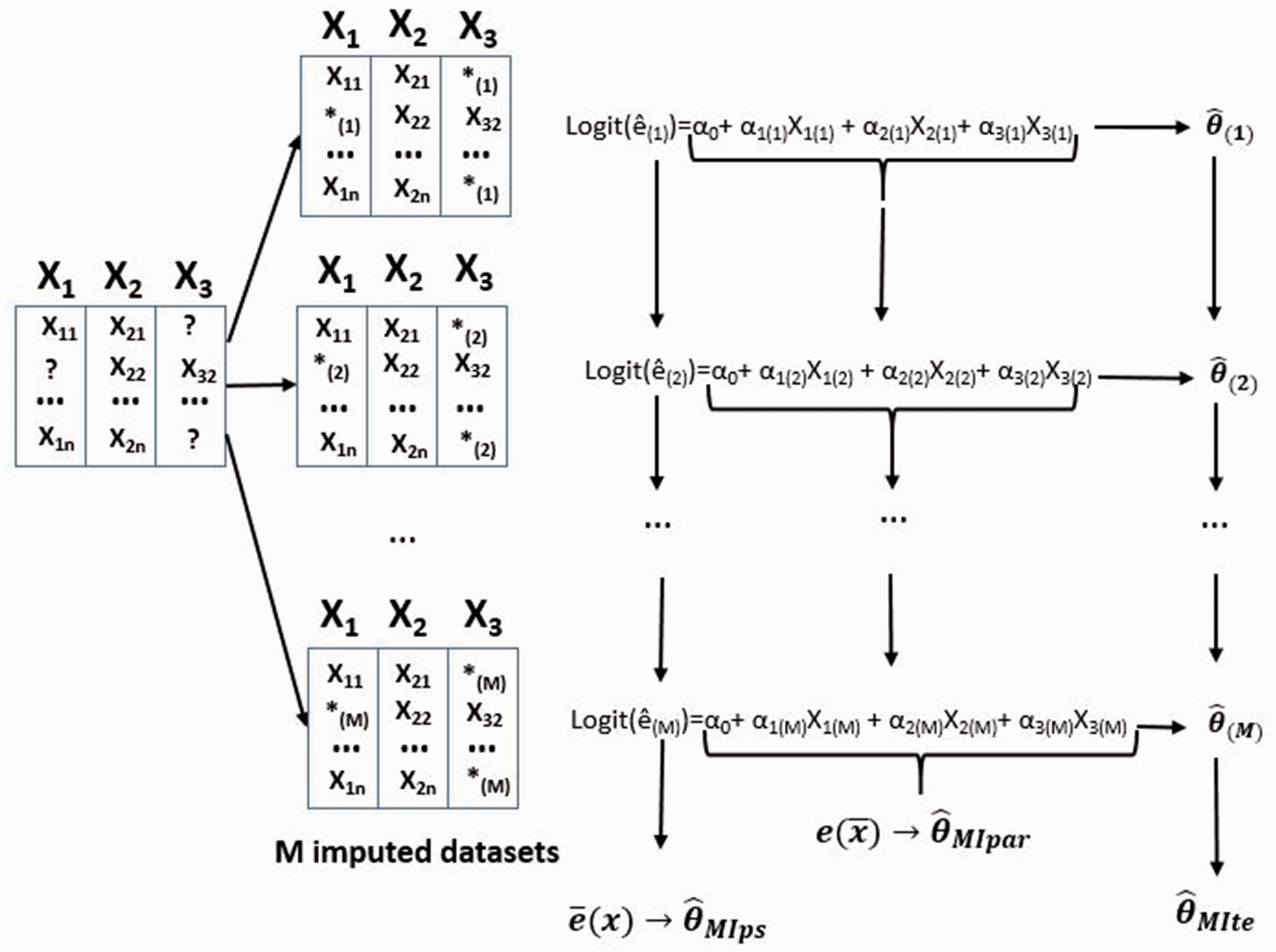Therefore, we focused on chained equations, in which a specific imputation model, including the outcome, is specified for each partially observed variable, rather than joint modelling to impute the missing data.³⁸ M complete datasets are created and analysed independently to produce estimates ${\hat{θ}}_{k}, (k = 1, \dots, M)$ of $θ$ the vector of the parameters of interest (e.g. regression coefficients) and estimates $W_{k}$ of their associated variance matrix. Then ${\hat{θ}}_{k}$ and $W_{k}, (k = 1, \dots, M)$ are combined across the M imputed datasets. Rubin’s rules for the mean and variance state that an overall estimate, ${\hat{θ}}_{MI}$ , of $θ$ and an estimate of the variance of ${\hat{θ}}_{MI}, \hat{Var} ({\hat{θ}}_{MI})$ , are⁸:

{\hat{θ}}_{MI} = \frac{1}{M} \sum_{k = 1}^{M} {\hat{θ}}_{k}, \hat{Var} ({\hat{θ}}_{MI}) = W + (1 + \frac{1}{M}) B,

(2)

where W is the within-imputation variance–covariance matrix, which reflects the variability of the parameter estimates in each imputed dataset, and B is the between-imputation variance matrix reflecting the variability in the estimates caused by the missing information. These two components are defined as:

W = \frac{1}{M} \sum_{k = 1}^{M} W_{k}, B = \frac{1}{M - 1} \sum_{k = 1}^{M} ({\hat{θ}}_{k} - {\hat{θ}}_{MI})^{2}

(3)

Three variants of MI are MIte, MIps and MIpar. For complete data, the IPTW method involves three steps: (a) estimation of the parameters α in the PS model; (b) calculation of individual PS’s; and (c) use of equation (1) to calculate ${\hat{μ}}_{0}$ and ${\hat{μ}}_{1}$ . In MIte, all three steps are applied to each of the M imputed datasets separately. Then the M treatment effect estimates obtained are averaged. In MIps, the method recommended by Mitra and Reiter,⁹ the first two steps are applied to each imputed dataset separately. Then the M PS’s for each individual are averaged and equation (1) is applied once using these average PS’s. In MIpar, the first step is applied separately to each of the imputed datasets. The M values of α and each individual’s covariates X_i are then averaged over the M datasets. Each individual’s PS is then estimated as: where $(i = 1, \dots, n)$ with $\bar{α}$ the $(p + 1)$ vector of the average PS parameter values (for the p covariates and the intercept) and ${\bar{x}}_{i}$ a $(p + 1)$ vector of the average p covariates across imputed datasets for individual i. Whereas the MIps estimate of treatment effect is based on the average PS, ${\bar{e}}_{i} (x_{i})$ , the MIpar estimate is based on the PS corresponding to the average of the covariates, ${\hat{e}}_{i} ({\bar{x}}_{i})$ . Rubin’s Rules are based on the assumption that ${\hat{θ}}_{k}$ is approximately normally distributed, and the distribution of $\hat{α}$ might be expected to be more approximately normal than the distribution of a PS (which is constrained to lie in [0,1]). The three MI approaches are illustrated in Figure 1. To obtain a variance estimator for the MIte estimator, Rubin’s rule for the variance (above) can be applied to the standard IPTW variance estimator for full data, which takes account of the PS estimation. For MIps and MIpar, because the PS is obtained from M imputations, the standard variance estimator for IPTW is no longer valid, since it does not take into account the uncertainty due to missing data. A large-sample estimate of the variance for MIpar, derived from Williamson et al.,³⁴ is given in Appendix 1.

Figure 1.

The three approaches considered after multiple imputation (MI) of the partially observed covariates are missing values on the original dataset. $*_{(k)}, (k = 1, \dots,, M)$ are imputed values in the kth imputed dataset. ${\hat{θ}}_{(k)}$ and ${\hat{e}}_{(k)}$ are the estimated treatment effect and estimated propensity scores, respectively, from the kth imputed dataset $(k = 1, \dots,, M)$ . The MIte approach consists of pooling the M treatment effects estimated with IPTW on each imputed dataset. MIps estimate is obtained by using the average PS across the M imputed datasets in the IPTW estimator. Finally, the MIpar approach uses the PS of the average covariate value across the M imputed dataset. The PS is estimated using the average PS parameters as regression coefficients.

5 Balancing properties and consistency of IPTW estimator after MI

Without missing data, Rosenbaum and Rubin showed that the PS is a balancing score.³ A balancing score $b (x)$ is defined as a function of the observed covariates x such that the conditional distribution of x given $b (x)$ is the same for Z = 0 and Z = 1. Moreover, Rosenbaum and Rubin showed that any balancing score $b (x)$ is ‘finer’ than the true PS, that is $e (x) = f {b (x)}$ , for some function $f (.)$ . The consistency of PS estimators comes from this balancing property. Lunceford and Davidian³⁵ studied theoretical properties of the IPTW estimator when data are complete and gave a proof of consistency of this estimator. In this section, we study the consistency of the IPTW estimators obtained from MIte, MIps and MIpar and how this relates to balancing properties of the PS models used in these approaches. We suppose hereafter that (a) the SITA assumption required for IPTW (see Section 3.1) holds, (b) the missing data are missing at random (MAR) and (c) the imputation model is correctly specified. For simplicity, we consider here the estimation of $θ = E [Y^{Z = 1}] .$

5.1 Combining the treatment effects after MI (MIte)

Let X, the vector of covariates, be split into observed and missing components, $X = (X_{obs}, X_{miss})$ . $X_{m}^{(k)}$ is the imputed value of $X_{miss}$ in the kth imputed dataset ( $k = 1, \dots, M$ ). We show (see Appendix 2a) that in each imputed dataset:

e (X_{obs}, X_{m}^{(k)}) = E [Z | X_{obs}, X_{m}^{(k)}]

(5)

If $X_{m}^{(k)}$ is imputed from the true model (i.e. correctly specified at the true parameter values), we can also show (Appendix 2b) that a SITA-type assumption holds in each imputed dataset, i.e.:

Y^{z = 1} ⊥ Z | X_{obs}, X_{m}^{(k)} and Y^{z = 0} ⊥ Z | X_{obs}, X_{m}^{(k)}

These two assumptions are the imputed-data version of what Imbens calls weak unconfoundedness.³⁹ Note that we do not have the analogue of the usual, stronger, assumption $(Y^{z = 1}, Y^{z = 0}) ⊥ Z | X_{obs}, X_{m}^{(k)}$ , which requires the treatment to be independent of the set of potential outcomes. This is because our imputation model is a model for $X_{miss} | Z = z, Y^{Z = z}, X_{obs}$ . The stronger assumption would require our imputation model to capture $X_{miss} | Z = z, Y^{z = 0}, Y^{z = 1}, X_{obs}$ . However, it is important to note, as Imbens does, that the weak unconfoundedness suffices to obtain unbiased estimates of the causal treatment effect.

5.1.1 Balancing properties

We show in Appendix 2 that $X_{obs} ⊥ Z | e (X_{obs}, X_{m}^{(k)}) and X_{m}^{(k)} ⊥ Z | e (X_{obs}, X_{m}^{(k)}) .$ Thus the true PS in each completed dataset balance both the unobserved and the imputed values of the covariates across treatment groups. This balancing property is what leads to consistency of the MIte estimator.

5.1.2 Consistency

Seaman and White¹¹ proved that for an infinite number of imputations, the estimator obtained by combining the treatment effects after MI (MIte) is consistent. To understand how this consistency relates to the SITA-type assumption above, it is helpful to consider the following expectation:

\begin{array}{l} E [\frac{Y Z}{e (X_{o b s}, X_{m}^{(k)})}] = E [E [\frac{Y Z}{e (X_{o b s}, X_{m}^{(k)})} | X_{o b s}, X_{m}^{(k)}]] \\ = E [\frac{E [Y^{z = 1} | X_{o b s}, X_{m}^{(k)}] E [Z | X_{o b s}, X_{m}^{(k)}]}{e (X_{o b s}, X_{m}^{(k)})}] \end{array}

(6)

\begin{array}{l} = E [E [Y^{z = 1} | X_{o b s}, X_{m}^{(k)}]] \\ = E [Y^{z = 1}] = θ, \end{array}

(7)

Step 6 requires the SITA-type assumption 6. Step 7 relies on PS in the kth imputed dataset being equal to the probability of being treated given the observed and imputed part of the covariates (equation 5).

5.2 Combining the PS or the PS parameters after MI (MIps and MIpar)

For PS methods, consistency comes from the ability of PS to balance covariates between groups. MIps and MIpar create a single overall PS used to estimate the treatment effect. Thus, consistency for these methods would rely on the ability of these overall PS to balance both the observed and the missing parts of the covariates in the original incomplete dataset. Rosenbaum and Rubin’s results show that this can happen only if the single PS (as estimated in MIps or MIpar) is ‘finer’ than the true (full data) PS (in other words, if the true PS is a function of the single pooled PS).³ However, when combining the PS or the PS parameters, the overall PS used for the analysis is not a function of the observed covariates but rather is a function of the average covariates across imputed datasets, including the imputed values. Thus, the pooled PS (as estimated either in MIps or MIpar) is not ‘finer’ than the true PS according to Rosenbaum and Rubins definition (i.e. the true PS is not a function of the pooled PS). Consequently, it cannot be a balancing score. Thus, neither ${\hat{θ}}_{MIps}$ nor ${\hat{θ}}_{MIpar}$ are consistent estimators. We illustrate the lack of consistency with a counter example in Appendix 3. We also discuss the balancing properties of the MP approach in Appendix 4.

6 Simulation study design

The aim of this simulation study is to assess the performance of the three MI approaches, CC analysis and missingness pattern approach for IPTW when the outcome is binary and to compare them with non-MI methods.

6.1 Data generation mechanisms

We generated datasets of sample size n = 2000, reflecting an observational study comparing a treatment Z = 1 to a control treatment Z = 0 on a fully observed binary outcome Y with three measured covariates $X = (X_{1}, X_{2}, X_{3})$ . X₁ and X₂ were continuous and X₃ was binary. X₂ was fully observed whereas X₁ and X₃ were partially observed. We generated the data as follows:

Covariates: The three covariates $X = (X_{1}, X_{2}, X_{3})$ are generated from a multivariate normal distribution $X \sim N_{3} (0, Σ)$ , with $Σ_{ii} = 1$ and $Σ_{ij} = ρ$ for $i \neq j$ . X₃ is then dichotomised according to a threshold of 0 to obtain a prevalence of 0.5.

Treatment assignment depends on X according to the following model:

logit (p (Z = 1 | x)) = - 1.15 + 0.7 x_{1} + 0.6 x_{2} + 0.6 x_{3}

(8)

These coefficients give

E (Z) = p_{Z} = 0.3

and an important imbalance on covariates between treatment groups, as shown in Appendix 6.

Binary outcome: The outcome depends on the three covariates and the treatment received according to the following model:

logit (p (Y = 1 | Z, x)) = - 1.5 + 0.5 x_{1} + 0.5 x_{2} + 0.3 x_{3} + θ_{c} Z

(9)

In this model,

\exp θ_{c}

is the conditional odds ratio (OR). We used the method described in Austin⁴⁰ to find the value of θ_c that gives the desired relative risk (RR).

Missingness mechanism: In this simulation study, we consider a MAR mechanism. The missingness of each partially observed covariate (X₁ and X₃) depends on the fully observed covariate X₂, the treatment received Z and the outcome Y:

logit (p (M_{1} = 1 | Z, x_{1}, x_{2}, x_{3}, y)) = γ_{0} + z + x_{2} + γ_{Y} y

(10)

logit (p (M_{3} = 1 | Z, x_{1}, x_{2}, x_{3}, y)) = γ_{0} + z + x_{2} + γ_{Y} y

(11)

where M₁ and M₃ are the missingness indicators for X₁ and X₃ (equal to 1 if the value is missing), respectively.

The values considered for each simulation parameter are in Table 1. A full factorial design (

2 \times 2 \times 2

) leads to eight scenarios, but five scenarios are added as a sensitivity analysis (Table 2).

Table 1.

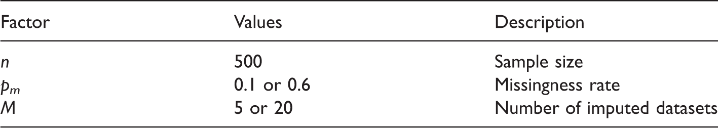
Factors used in the simulation study ( $2 \times 2 \times 2$ factorial design).

Factor	Values	Description	Comments
ρ	0.3 or 0.6	Correlation between the covariates	After dichotomization, $corr (X_{1}; X_{3}) =$ $corr (X_{2}, X_{3}) = 0.24$ or 0.46
RR	1 or 2	Relative risk	In model (9), $θ_{c} = 0$ or 1.221 when $ρ = 0.3$ , and 0 or 1.289 when $ρ = 0.6$ .
γ_Y	0 or −0.4	Association between the outcome and the probability of missingness	When $γ_{Y} = 0, γ_{0} = - 1.5$ and when $γ_{Y} = - 0.4, γ_{0} = - 1.3$ in model (10) and (11)

For each scenario, 5000 datasets of sample size 2000 were generated. The prevalence of the treatment was 0.3 and each partially observed covariate had 30% of data missing. Ten imputed datasets were created.

Table 2.

Simulation parameters used for the sensitivity analysis.

Factor	Values	Description
n	500	Sample size
p_m	0.1 or 0.6	Missingness rate
M	5 or 20	Number of imputed datasets

For each scenario of the sensitivity analysis, 5000 datasets were generated. The other parameter values were: RR = 2, $ρ = 0.6$ and $γ_{Y} = - 0.4$ .

6.2 Methods

For each studied scenario, 5000 datasets were simulated. We compared nine methods, all of them using IPTW: treatment effect were estimated on the full dataset (before the imposition of missingness) and using CC, MP, and the three MI approaches (MIte, MIps and MIpar). For each of the three MI approaches, we considered two imputation models, including or not the outcome and we generated M = 10 imputed datasets. Simulations were performed in R and the mi package was used for MI,⁴¹ based on full conditional specification (FCS).

6.2.1 Estimands

We focused on three estimands: the log(RR), log(OR) and the risk difference (RD). Rubin’s rules were applied to the logarithm of the RRs (or the ORs), rather than to RRs (or ORs) themselves, because the asymptotic normal approximation is likely to be better for the log RR (or log OR) than for the RR (or OR). This is important in particular when constructing confidence intervals, because log(OR) and log(RR) have unrestricted parameter spaces.⁴²

6.2.2 Measures of performance

For each method, we computed the absolute bias of the mean treatment effect. We also estimated the variance of the treatment effect, as well as the empirical variance, the coverage rate and the standardized differences of the covariates after IPTW.

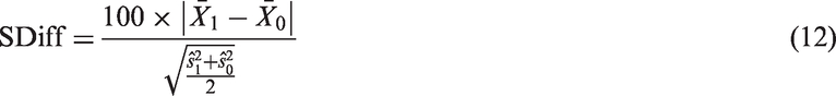
The standardized differences for each covariate were used as a measure of method performance. In the absence of weighting, standardized differences are defined as:

SDiff = \frac{100 \times | {\bar{X}}_{1} - {\bar{X}}_{0} |}{\sqrt{\frac{{\hat{s}}_{1}^{2} + {\hat{s}}_{0}^{2}}{2}}}

(12)

with

{\bar{X}}_{0}, {\bar{X}}_{1}, {\hat{s}}_{0}^{2}

and

{\hat{s}}_{1}^{2}

denoting the average value (or proportion if the covariate is binary) for the covariate and its estimated variance in the control and treatment group, respectively. After IPTW, standardized differences are calculated by replacing the unweighted means and variances in (12) by their weighted equivalents (weighted by inverse PS). For the MIte approach, standardized differences were calculated using the PS estimated from each imputed dataset, both to assess the balance on the originally simulated complete dataset (before imposing missingness) and on the given imputed dataset. For MIps and MIpar, standardized differences were calculated using the pooled PS to assess balance on (a) the original dataset, (b) on the average value of the covariates across the imputed datasets. For (b) we also calculated the standardized differences separately on the observed part of the covariates and the average imputed part.

7 Simulation study results

7.1 Main simulation study

Because results were similar for the three measures of interest, we present the results for relative risks (RR) on the log scale only in the main text, while results for odds ratios and risk differences are in the appendices.

7.1.1 Bias

The absolute bias of the log(RR) of the treatment, for $ρ = 0.6$ , is presented in Figure 2. Since results for $ρ = 0.3$ are similar, they are presented in the Appendices.

Figure 2.

Absolute value of the bias for the four scenarios in which 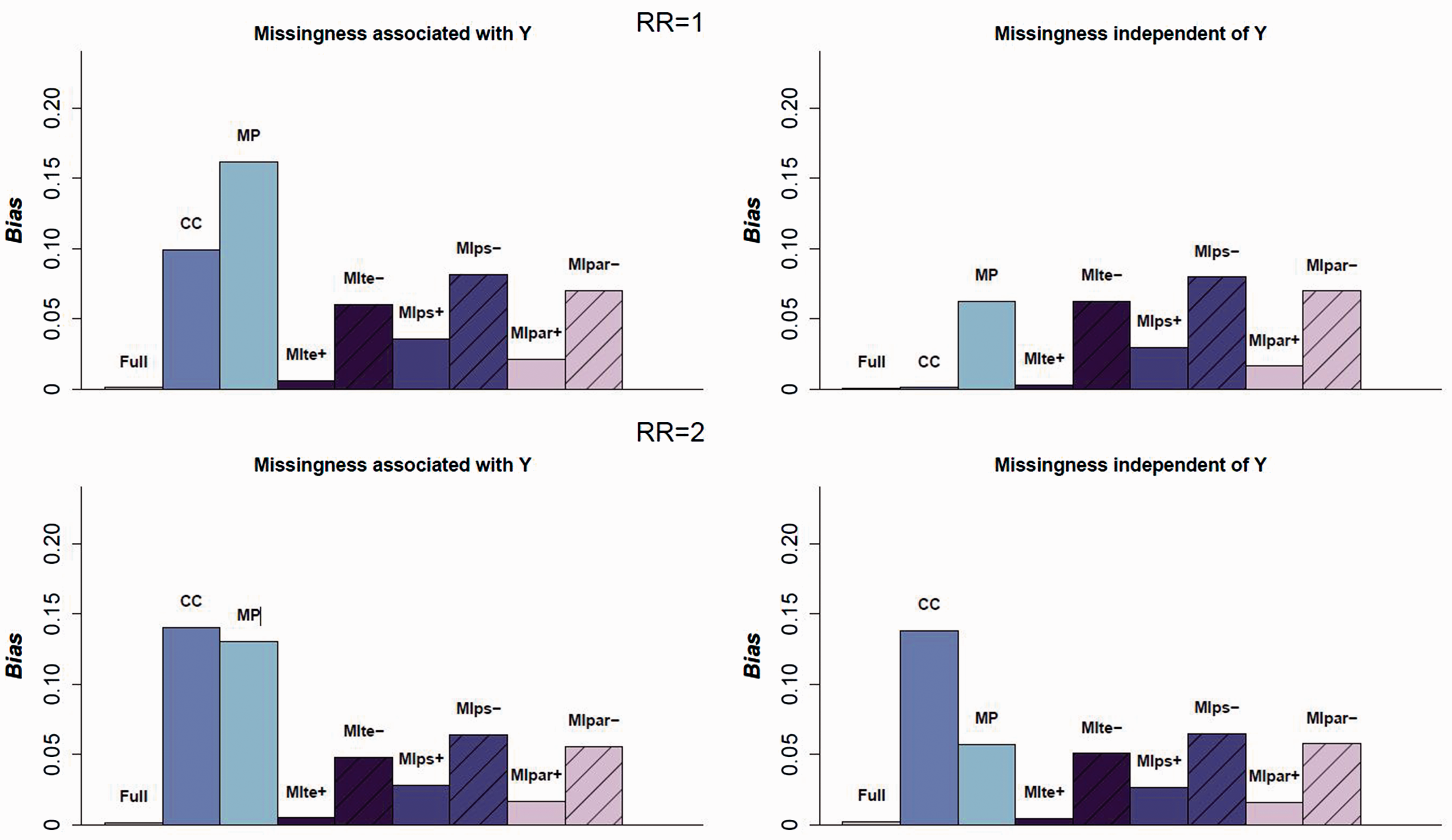$ρ = 0.6$ . CC: complete case; MP: missingness pattern; MIte: treatment effects combined after multiple imputation; MIps: propensity scores combined after multiple imputation; MIpar: propensity score parameters combined after multiple imputation. For the three MI approaches ‘+’ means that the outcome is included in the imputation model, ‘−’ means that the outcome is not in the imputation model. RR: relative risk.

Full data, CC and MP analyses

As expected, the IPTW estimator on the full data (before generating missingness for X₁ and X₃) is approximately unbiased and the CC estimator is strongly biased in all scenarios except those where the outcome is not associated with missingness and there is no treatment effect. The MP approach is always biased in the situations considered, with a bias which can be even stronger than that which is observed for the CC approach. The reason for this is an incorrect PS model specification in each pattern of missingness: in the strata in which a covariate is not observed, the covariate is omitted from the model.

MI

First, the results show that the imputation model must include the outcome, even if the outcome is not a predictor of missingness. All three MI estimators are strongly biased in all scenarios when the outcome is not included in the imputation model. Second, when the outcome is included in the imputation model, the three MI approaches lead to a decrease in bias relative to the crude analysis. However, only the MIte approach leads to an unbiased estimate in the eight main scenarios. Combining the PS parameters to estimate the PS of the average covariates (MIpar) performed better than combining the PS themselves, but both these approaches are slightly biased.

7.1.2 Standardized differences between groups

The bias observed for the MP, MIps and MIpar methods can be explained by a remaining imbalance on the covariates between groups. Standardized differences for each covariate are in Table 3. A covariate is usually considered adequately balanced if its standardized difference is

< 10 %

. IPTW on the full data achieved a very good balance between groups on the three covariates (as expected, standardized difference <5% for each of the three covariates). For the CC approach, groups were balanced but the bias occurs since excluded individuals are different from included individuals on confounding factors. The PS obtained from the MP approaches balanced the observed part of the covariates, but not the unobserved part. This means that within each pattern of missingness, treated and untreated individuals are balanced for the covariates included in the PS model, but unbalanced on the missing covariate because this covariate is an unmeasured confounder in the PS model. Thus, when the missingness rate increases, imbalances (and consequently, bias of the treatment effect estimate) increase. MIte performs well because the PS within each imputed dataset balances the observed and imputed components of the covariates in that imputed dataset (see Table 3). Conversely, MIps and MIpar could only be consistent by balancing the observed and missing covariates, which is not the case, as seen in Table 3.

Table 3.

Standardized differences (in %) after IPTW for each method for one scenario: RR = 2, $ρ = 0.6$ , outcome predictor of missingness and included in the imputation model (n = 2000).

Method	X1	X2	X3
Crude (without IPTW)	81.3	74.7	51.7
Full	4.6	4.6	2.4
CC (n = 1074)	7.6	7.3	3.5
MP
Balance on full data	14.6	4.3	8.5
Balance on the observed part of the covariate	6.1	4.3	2.9
Balance on the missing part of the covariate	48.6	NA	28.3
MIte
Balance on full data	15.0	4.5	9.1
Balance on each imputed dataset	4.5	4.5	2.4
MIps
Balance on full data	15.9	5.5	10.7
Balance on the average imputed dataset	15.8	5.5	10.6
Balance on the observed part of the covariate	7.6	5.5	4.9
Balance on the imputed part of the covariate	58.1	NA	36.9
MIpar
Balance on full data	15.1	4.8	9.6
Balance on the average imputed dataset	14.7	4.8	9.7
Balance on the observed part of the covariate	7.7	4.8	5.4
Balance on the imputed part of the covariate	52.5	NA	34.3

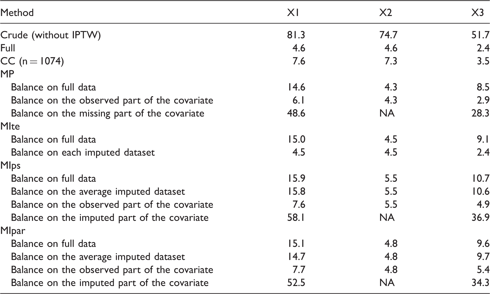
CC: complete case; MP: missingness pattern; MIte: treatment effects combined after multiple imputation; MIps: propensity scores combined after multiple imputation; MIpar: propensity score parameters combined after multiple imputation; RR: relative risk; NA: not applicable because X₂ is fully observed.

7.1.3 Coverage rate and standard errors

Figure 3 displays the coverage rate for each method when the outcome is included in the imputation model. Each boxplot represents the coverage distribution for the eight main scenarios. Because the CC and MP approaches are strongly biased, their coverage rates are not relevant. The coverage rate for the MIte approach is close to the nominal value of 95%, confirming that Rubin’s rules perform well in this context provided that the within-imputation variance estimation takes into account the uncertainty in PS estimation (Table 4).

Figure 3.

Coverage rate of the 95% CI for each method compared. Results are pooled for the 8 main scenarios. CC: complete case; MP: missingness pattern; MIte: treatment effects combined after multiple imputation; MIps: propensity scores combined after multiple imputation; MIpar: propensity score parameters combined after multiple imputation. RR: relative risk. For the three MI methods, the outcome is included in the imputation model.

Table 4.

Bias of the log(RR), its estimated variance and coverage rate for the three MI approaches according the sample size n for one scenario (RR = 2, $ρ = 0.6$ , outcome predictor of missingness and included in the imputation model). Results based on 5000 simulations.

	Full		CC		MP		MIte		MIps		MIpar
	n = 500	n = 2000	n = 500	n = 2000	n = 500	n = 2000	n = 500	n = 2000	n = 500	n = 2000	n = 500	n = 2000
Bias	0.007	0.002	0.110	0.141	0.153	0.130	0.010	0.005	0.038	0.028	0.024	0.017
Variance	0.022	0.006	0.050	0.014	0.029	0.008	0.026	0.007	0.022	0.006	0.023	0.006
Empirical variance	0.024	0.006	0.059	0.014	0.027	0.007	0.025	0.006	0.024	0.006	0.025	0.006
Coverage rate	0.940	0.947	0.887	0.769	0.855	0.691	0.955	0.957	0.939	0.932	0.943	0.942

MIte: treatment effects combined after multiple imputation; MIps: propensity scores combined after multiple imputation; MIpar: propensity score parameters combined after multiple imputation.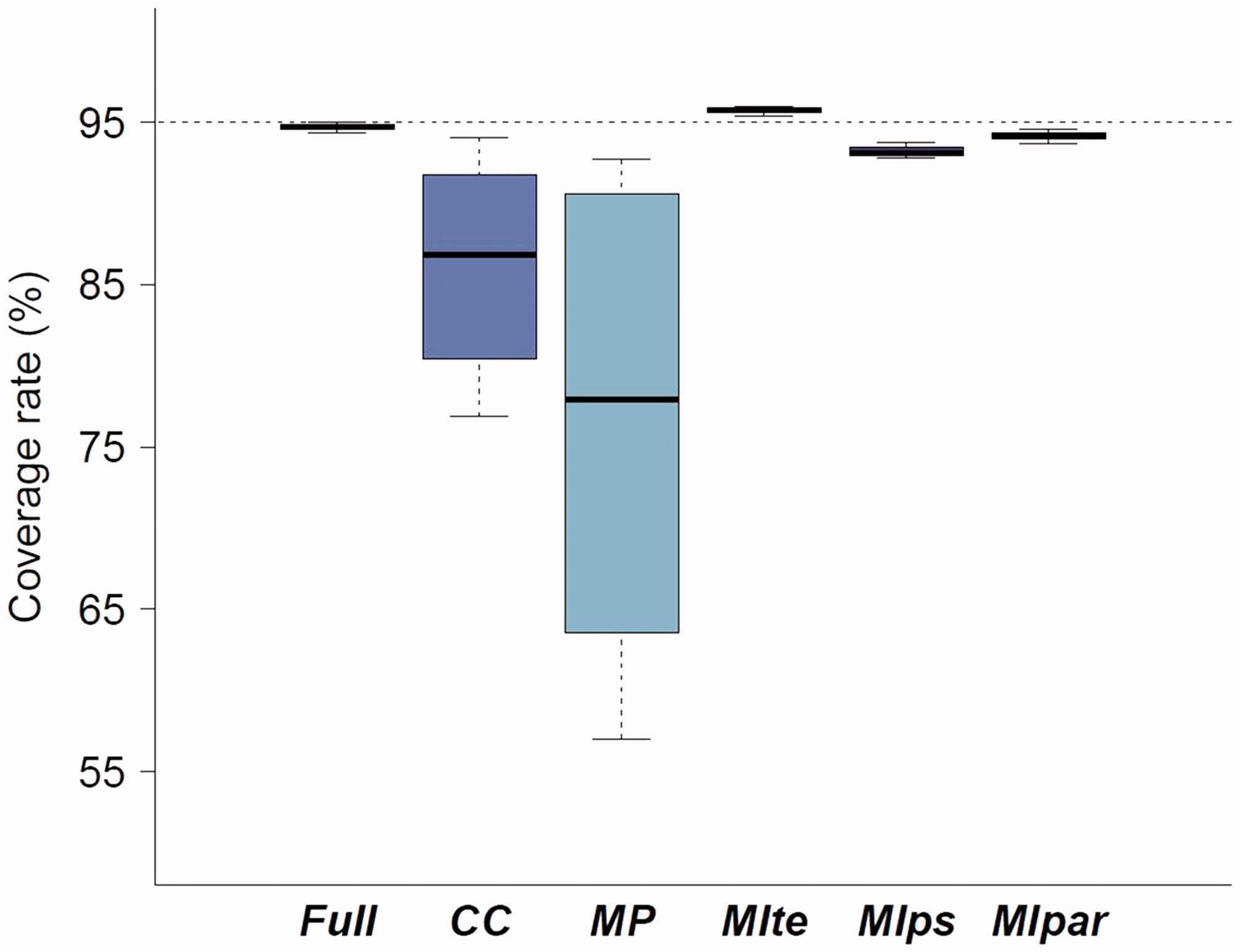

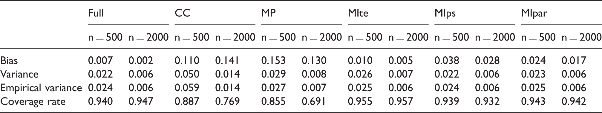
Table 1 in Appendix 5.1 shows the mean estimates from different variance estimators for each method when the outcome is included in the imputation model. For MIte, one could apply Rubin’s rules to a variance estimator that ignores the PS estimation (treating the PS weights as being known) or to a variance estimator that accounts for the PS estimation. We know that failing to account for the PS estimation results in an overestimation of the variance in the full-data context.⁴³ Table in Appendix 5.1 shows that for the analysis on full data and for MIte, the variances accounting for PS estimation are close to the empirical variance, whereas an estimator not taking the uncertainty in PSs estimation tends to overestimate the variance for these approaches, as expected. For MIps and MIpar, one could estimate the variance accounting for the variability linked to PS estimation but not the imputation procedure by using the pooled PS in the IPTW variance estimator or one could incorporate the PS estimation and imputation by applying the variance estimator we proposed in Appendix 1. For MIps and MIpar, there was little difference between the variance estimates accounting for the imputation and those that did not. Surprisingly, in our simulations, additionally accounting for the imputation procedure resulted in a lower variance estimator. This can be explained as follows: the within imputation variance of the PS parameters (reflecting the correlation between the covariates and treatment; the higher this is the larger gain in precision for IPTW) is higher than the between imputation variance component (noise due to missing data). However, when the missingness rate increases, the variance that correctly accounts for the imputation procedure is typically higher than the variance which ignores the imputation, because of a larger heterogeneity between imputed datasets.

7.2 Sensitivity simulation study

Appendix 5.3 presents the results of one scenario with a non-null treatment effect with a smaller sample size (n = 500). Results were similar in terms of bias for n = 500 and n = 2000. Because the variance estimator for IPTW has been developed for large samples, we observed slightly underestimated variances for the full data analysis, MIps and MIpar. This underestimation is more pronounced in the CC analysis because the sample for the analysis is even smaller (269 on average when n = 500).

Figure 4 shows the bias when 10% or 60% of each partially observed covariate is missing. Full results are presented in Appendix 5.4. For a low missingness rate, the CC and MP approaches are still biased but the three MI approaches corrected the bias. For a missingness rate of about 60% for each covariate, only the MIte approach showed good performance in terms of bias reduction, confirming the good statistical properties of this approach even with this large amount of missing data. In our sensitivity simulation study, increasing the number of imputed datasets did not strongly impact the results in terms of bias or variance (See Appendix 5.5).

Figure 4.

Absolute value of the bias according to the missingness rate. CC: complete case; MP: missingness pattern; MIte: treatment effects combined after multiple imputation; MIps: propensity scores combined after multiple imputation; MIpar: propensity score parameters combined after multiple imputation; RR: relative risk. For the three MI methods, the outcome is included in the imputation model.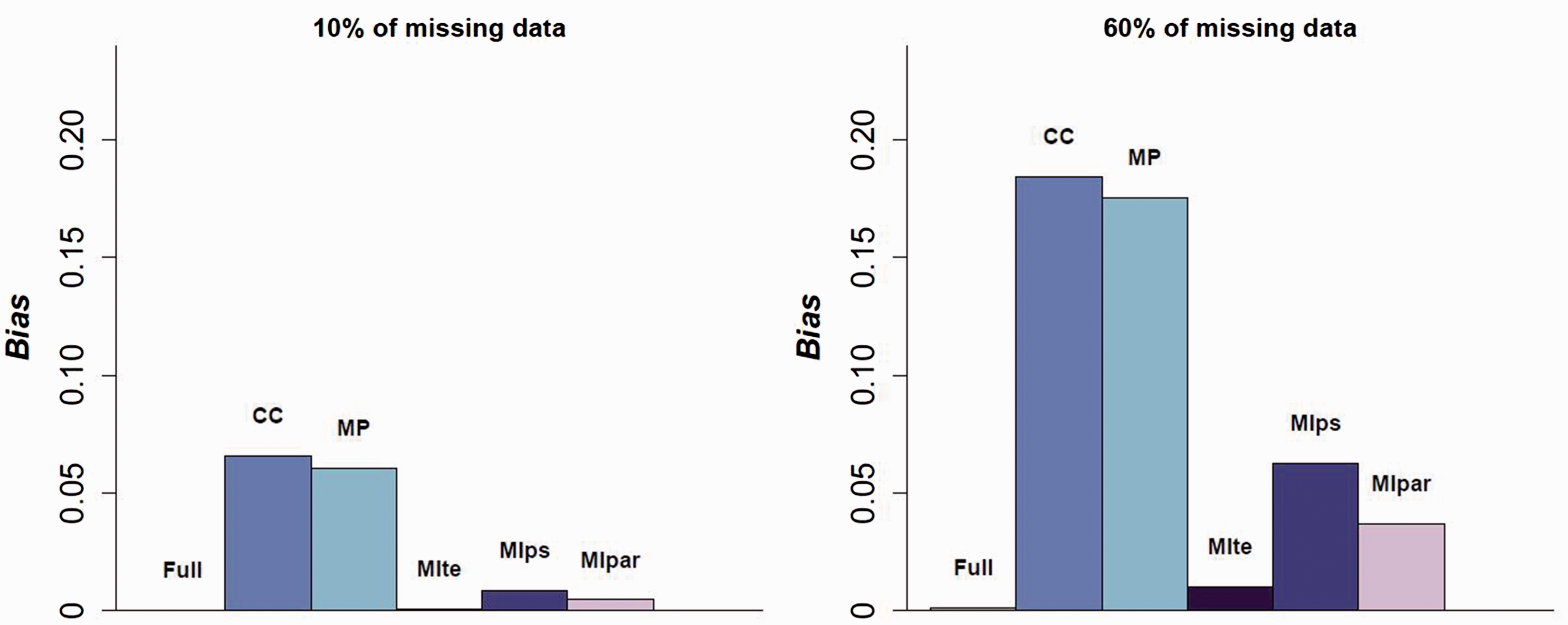

8 Application to the motivating example

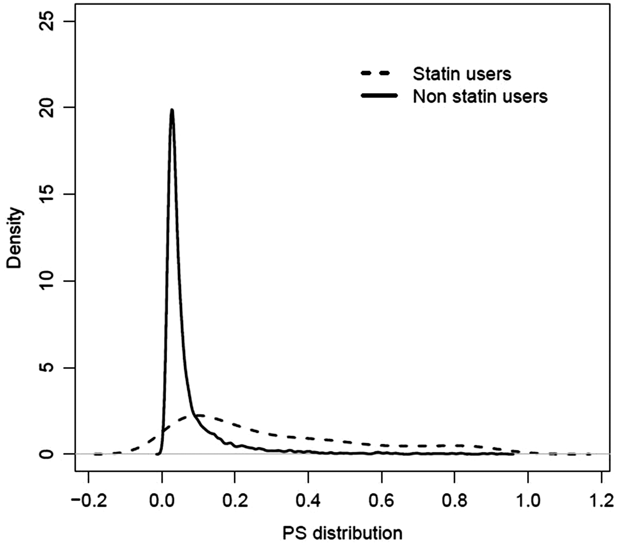
We applied CC analysis, the MP approach and the three MI strategies to estimate the effect of statin treatment on mortality after pneumonia from our motivating example dataset. For simplicity, we analysed the primary outcome, mortality within 6 months, as a binary outcome, and estimated the corresponding relative risk and its 95% confidence interval. For each approach, IPTW was used to account for the confounding. We focused the analysis on the 7158 patients without coronary heart disease. The PS was estimated from a logistic regression modelling statin use as a function of the following covariates: age, sex, body mass index (BMI), alcohol consumption, smoking status, diabetes, cardiovascular disease, circulatory disease, heart failure, dementia, cancer, hyperlipidaemia, hypertension and prescription of antipsychotics, hormone replacement therapy, antidepressants, steroids, nitrates, beta-blockers, diuretics, anticoagulants and use of antihypertensive drugs. The imbalance between the study groups is illustrated in Figure 5. Complete case (CC) analysis was conducted on the 5168 individuals with complete records. For the missingness pattern approach (MP), eight patterns were identified. However, some of these patterns were very rare. For instance, only six individuals had only the smoking status missing, and only eight had both smoking status and BMI missing. Thus, we considered only four groups:

complete records (n = 5168) for which all the covariates listed above are included

individuals with only the alcohol consumption missing (n = 455)

individuals with only BMI missing (n = 575)

individuals with the smoking status missing (alone or in addition to BMI and alcohol consumption) and individuals with both BMI and alcohol consumption missing (n = 960)

Figure 5.

Distribution of the propensity score estimated on complete cases for statin users and non users (n = 5168).

For MI, 10 imputed datasets were created. The imputation model included statin use, mortality and all the variables listed above. The standardized differences estimated before weighting and after weighting by PS for CC, MP, MIte, MIps and MIpar are presented in Table 5. The MP and the three MI approaches lead to a similar reduction in imbalance between groups on the observed variables as compared to the crude standardized differences. Nevertheless, because of the poor overlap of the patients characteristics between groups (Figure 5), some covariates are still unbalanced even after MI. However, for binary covariates, large standardized differences can occur even for slight imbalance when the prevalence is low. Estimated RRs are presented in Table 6. First, all approaches based on IPTW lead to a treatment effect estimate smaller than the unweighted treatment effect. The three MI approaches lead to similar RR and these were smaller than the RR obtained from CC and MP analyses. The small differences between the three MI approaches in this example can be explained by a low rate of missing data and the fact that the three partially observed covariates were not strong confounders.

Table 5.

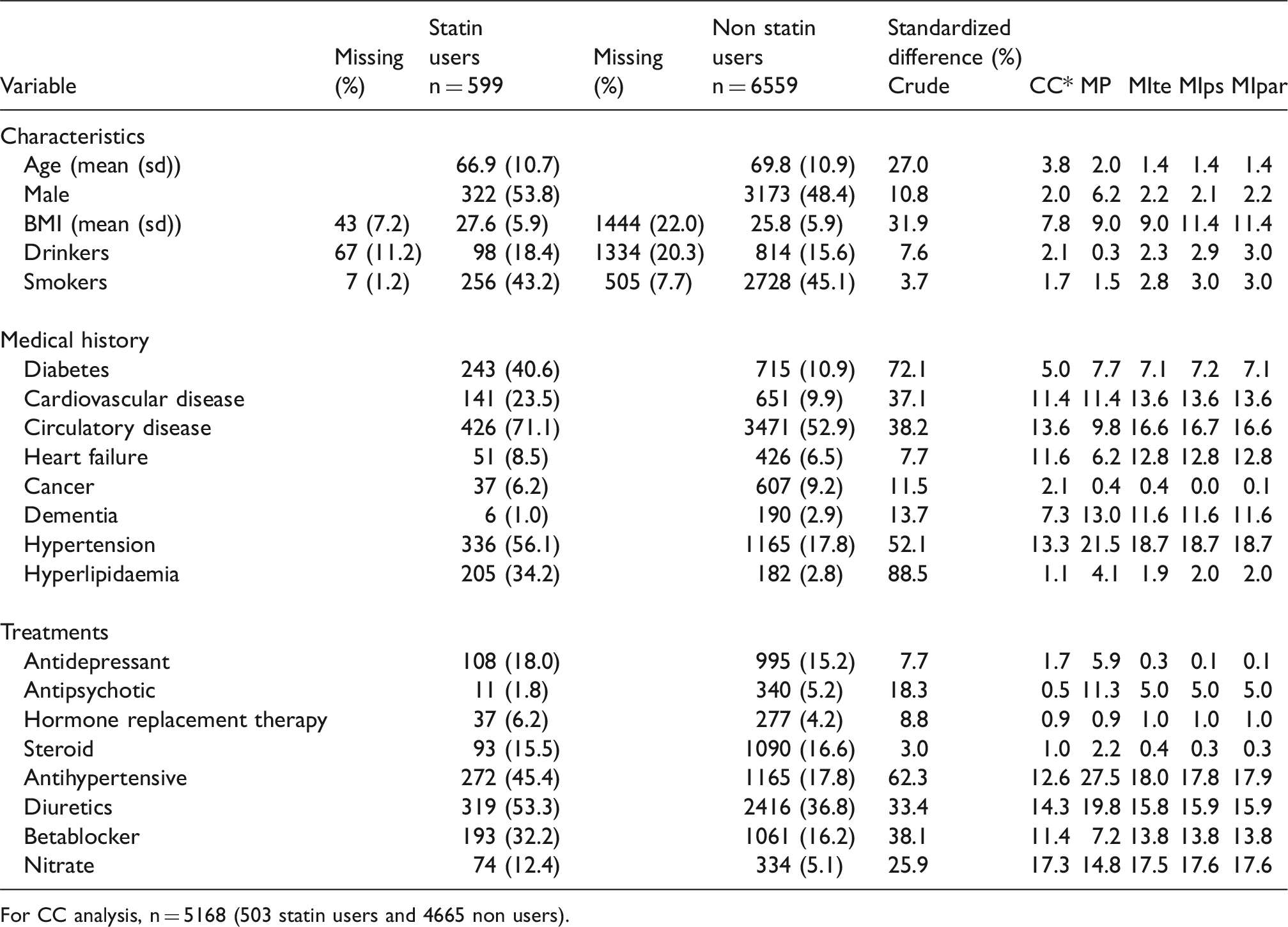
Description and comparison of statin users and non users (n = 7158).

Variable	Missing (%)	Statin users	Missing (%)	Non statin users	Standardized difference (%)
		n = 599		n = 6559	Crude	CC*	MP	MIte	MIps	MIpar
Characteristics
Age (mean (sd))		66.9 (10.7)		69.8 (10.9)	27.0	3.8	2.0	1.4	1.4	1.4
Male		322 (53.8)		3173 (48.4)	10.8	2.0	6.2	2.2	2.1	2.2
BMI (mean (sd))	43 (7.2)	27.6 (5.9)	1444 (22.0)	25.8 (5.9)	31.9	7.8	9.0	9.0	11.4	11.4
Drinkers	67 (11.2)	98 (18.4)	1334 (20.3)	814 (15.6)	7.6	2.1	0.3	2.3	2.9	3.0
Smokers	7 (1.2)	256 (43.2)	505 (7.7)	2728 (45.1)	3.7	1.7	1.5	2.8	3.0	3.0

Medical history
Diabetes		243 (40.6)		715 (10.9)	72.1	5.0	7.7	7.1	7.2	7.1
Cardiovascular disease		141 (23.5)		651 (9.9)	37.1	11.4	11.4	13.6	13.6	13.6
Circulatory disease		426 (71.1)		3471 (52.9)	38.2	13.6	9.8	16.6	16.7	16.6
Heart failure		51 (8.5)		426 (6.5)	7.7	11.6	6.2	12.8	12.8	12.8
Cancer		37 (6.2)		607 (9.2)	11.5	2.1	0.4	0.4	0.0	0.1
Dementia		6 (1.0)		190 (2.9)	13.7	7.3	13.0	11.6	11.6	11.6
Hypertension		336 (56.1)		1165 (17.8)	52.1	13.3	21.5	18.7	18.7	18.7
Hyperlipidaemia		205 (34.2)		182 (2.8)	88.5	1.1	4.1	1.9	2.0	2.0

Treatments
Antidepressant		108 (18.0)		995 (15.2)	7.7	1.7	5.9	0.3	0.1	0.1
Antipsychotic		11 (1.8)		340 (5.2)	18.3	0.5	11.3	5.0	5.0	5.0
Hormone replacement therapy		37 (6.2)		277 (4.2)	8.8	0.9	0.9	1.0	1.0	1.0
Steroid		93 (15.5)		1090 (16.6)	3.0	1.0	2.2	0.4	0.3	0.3
Antihypertensive		272 (45.4)		1165 (17.8)	62.3	12.6	27.5	18.0	17.8	17.9
Diuretics		319 (53.3)		2416 (36.8)	33.4	14.3	19.8	15.8	15.9	15.9
Betablocker		193 (32.2)		1061 (16.2)	38.1	11.4	7.2	13.8	13.8	13.8
Nitrate		74 (12.4)		334 (5.1)	25.9	17.3	14.8	17.5	17.6	17.6

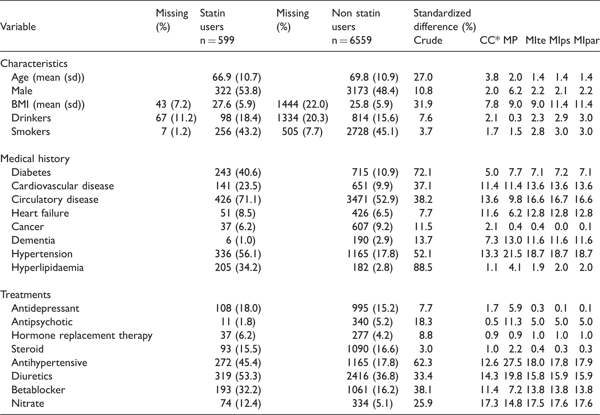
For CC analysis, n = 5168 (503 statin users and 4665 non users).

Table 6.

Estimate of the relative risk of mortality and its 95% confidence interval for statin vs non statin users (motivating example) (n = 7158).

Method	$\hat{RR}$	95% CI( $\hat{RR}$ )
Crude	0.587	[0.497;0.684]
CC	0.702	[0.534;0.924]
MP	0.708	[0.555;0.904]
MIte	0.654	[0.513;0.835]
MIps	0.653	[0.512;0.834]
MIpar	0.654	[0.513;0.834]

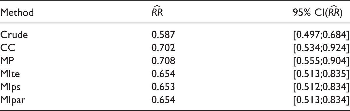
RR: relative risk; CC: complete case; MP: missingness pattern; MIte: treatment effects combined after multiple imputation; MIps: propensity scores combined after multiple imputation; MIpar: propensity score parameters combined after multiple imputation; RR: relative risk.

9 Discussion

This article aimed to address three main questions about MI in the context of IPTW: (a) does the outcome have to be included in the imputation model? (b) should we apply Rubin’s rules on the IPTW treatment effect estimates or on the PS estimates themselves? (c) how should we estimate the variance of the IPTW estimator after MI? First, results showed that the outcome must be included in the imputation model, even if the outcome is not a predictor of missingness. This is well known in the context of multivariable regression, but can be seen as counter-intuitive in the PS paradigm, because the PS model for the full data does not use the outcome data. The simulation results showed a bias in the three MI estimators when the outcome was omitted from the imputation model, even when the outcome was not a predictor of missingness. In practice, to obtain an unbiased estimate of the intervention effect when using MI, the outcome should be included in the imputation model. This may not be always possible if the outcome data has not been yet recorded and the PS is used at the design stage of the study (to find good matched controls for example), rather than at the analysis stage. In such situations, it is worth considering whether the assumptions required for CC analysis or the MP approach may be valid. If they are, one of these methods could be used instead of using MI omitting the outcome. Furthermore, the inclusion of the outcome in the imputation model may go against the principle of objective design, as described by Rubin.⁴⁴ However, when using MI, this is necessary to obtain a consistent estimator of the treatment effect. Second, we showed that combining the treatment effects after MI (MIte approach) is the preferred MI strategy in terms of bias reduction under a MAR mechanism. This estimator is the only estimator of the three MI estimators to be consistent and to provide good balancing properties. Even though MIps and MIpar are not consistent estimators of the treatment effect, they can reduce the bias of the CC analysis, if the rate of missing data is not too high. Combining the PS or the PS parameters has no clear advantage for IPTW, but may be useful in the context of PS matching: because it involves only one estimation of the treatment effect, it could provide a computational advantage for large datasets. In addition, MIte for PS matching implies that the M treatment effect estimates are estimated from different matched sets, potentially of different sample sizes, leading to a more complex variance estimation because of these different sample sizes.

Third, as long as the uncertainty in the PS estimation is taken into account in the variance estimation,³⁴ Rubin’s rules perform well for MIte, even for moderate sample size (n = 500). For MIpar, the proposed variance approximation (Appendix 1) showed good performance in our simulation study.

The three MI approaches differ in terms of their balancing properties. We showed that whereas the PS estimated in each dataset in the MIte approach can balance covariates between groups in each imputed dataset, this is no longer true for MIps and MIpar. However, the best method to assess covariate balance after MI remains unknown. With MIte, the aim being to estimate a treatment effect from each dataset, we require balance between groups within each imputed dataset. In contrast, for MIps and MIpar, further investigation is needed to know if we should assess the balancing properties of the pooled PS on the average covariate values across the imputed dataset or on each dataset.

Our recommendations for the optimal way to implement MI for PS analysis are in contradiction to those given by Mitra and Reiter, who suggest that pooling PSs across imputed datasets can sometimes out-perform our recommended method of pooling treatment effects.⁹ In their simulation studies MIps (or MIpar) led to a bigger reduction in bias than MIte in some scenarios. This was due to a near violation of the positivity assumption in their simulated datasets⁴⁵ combined with the omission of the outcome from the imputation model. Penning de Vries and Groenwold⁴⁶ used Mitra and Reiter’s data-generating mechanism to perform a simulation study but they increased the effective sample size to ensure positivity. Under this condition and when the outcome was included in the imputation model, as we recommend, they showed MIte was superior, in accordance with our findings. While we understand the desire to adhere to the principle of objective design by omitting the outcome from the imputation model, our results show that this leads to bias in MIte and an increase in bias for MIps (and MIpar). Thus, when it is either undesirable or impossible to include the outcome in the imputation model, we would suggest considering the validity of alternative approaches, such as CC analysis or the MP approach, rather than adopting the systematically biased approach of imputation omitting the outcome from the imputation model.

The MP approach, which is widely used in practice to handle missing data for PS analysis, showed poor performance under a MAR mechanism. In our simulation study, the MP approach does not perform well, because missing data were generated under a MAR mechanism, but the MP approach relies on different assumptions about the missing data mechanism.³⁷ When the assumptions for the MP approach are valid, it avoids the need for an imputation model altogether, and hence avoids the need to use the outcome when calculating the PS. Because the assumptions for MI and MP are different, we believe that MP could be a promising alternative when the assumptions for MI are not valid. Further investigations are needed to understand the usefulness of the MP approach in practice. Moreover, its application to our real-life example dataset was challenging, because the sample size within each missingness pattern was not large enough to estimate the PS.

This work has some limitations. We generated only three covariates in our simulation, whereas PS are often calculated from a large number of covariates. Moreover, we studied only the common situation where the PS model only includes main effects, and we assumed as well the model including main effects only for the outcome given the covariates. When there are interactions or quadratic terms in these two models, the specification of the imputation model can be less straightforward, requiring further efforts to ensure the imputation model is compatible with the substantive (analysis) model.⁴⁶ Furthermore, we focussed on the IPTW estimator only, because of its increasing use and its application in the presence of time-varying covariates and treatment. Indeed, IPTW is widely used in marginal structural models (MSMs) to handle time-dependent confounding. Although this article is about the simpler situation of a single time-point, it is important to clarify how to use IPTW after MI correctly in this context, because otherwise it is unlikely to be done correctly in the more complex situation of time-dependent confounding. However, some issues may arise with IPTW when some estimated weights are too extreme; PS matching can be a better solution in this context.⁴⁷ Nevertheless, because the PS estimated in either MIps or MIpar is not a balancing score, PS matching (like IPTW – and like also PS stratification and PS covariate adjustment) would not be expected to perform well when used in combination with MIPs or MIPar. Conversely, because in MIte, the estimated PS can balance both the observed and imputed component of the covariates in the imputed dataset, we would expect all the PS-based methods (PS matching, stratification, covariate adjustment and IPTW) to perform well to estimate the treatment effect within each imputed dataset as long as the underlying assumptions for these methods are fulfilled.

In conclusion, for IPTW, MI followed by pooling of treatment effect estimates is the preferred approach amongst those studied, when data are MAR, and the outcome must be included in the imputation model.

Footnotes

Declaration of conflicting interests

The author(s) declared no potential conflicts of interest with respect to the research, authorship, and/or publication of this article.

Funding

The author(s) disclosed receipt of the following financial support for the research, authorship, and/or publication of this article: This work was supported by the Medical Research Council (Project Grant MR/M013278/1 and Unit Programme Number U105260558).

Supplemental material

Supplemental material is available for this article online.

References

Concato

Shah

Horwitz

. Randomized, controlled trials, observational studies, and the hierarchy of research designs. New Engl J Med 2000; 342: 1887–1892.

Cochran

Rubin

. Controlling bias in observational studies: A review. Sankhyā: Indian J Stat Ser A (1961-2002) 1973; 35: 417–446.

Rosenbaum

Rubin

. The central role of the propensity score in observational studies for causal effects. Biometrika 1983; 70: 41–55.

Guo

. Propensity score analysis: statistical methods and applications, Thousand Oaks, CA: Sage Publications, 2009.

Hirano

Imbens

. Estimation of causal effects using propensity score weighting: An application to data on right heart catheterization. Health Serv Outcome Res Methodol 2001; 2: 259–278.

White

Carlin

. Bias and efficiency of multiple imputation compared with complete-case analysis for missing covariate values. Stat Med 2010; 29: 2920–2931.

Rosenbaum

Rubin

. Reducing bias in observational studies using subclassification on the propensity score. J Am Stat Assoc 1984; 79: 516–524.

Carpenter

Kenward

. Multiple imputation and its application, Chichester: John Wiley & Sons, 2012.

Mitra

Reiter

. A comparison of two methods of estimating propensity scores after multiple imputation. Stat Methods Med Res 2012; 0: 1–17.

10.

Mitra R and Reiter JP. Estimating propensity scores with missing covariate data using general location mixture models, http://eprints.soton.ac.uk/67154/ (2009, accessed 20 May 2017).

11.

Seaman

White

. Inverse probability weighting with missing predictors of treatment assignment or missingness. Commun Stat - Theory Methods 2014; 43: 3499–3515.

12.

Moons

KGM

Donders

RART

Stijnen

et al.

Using the outcome for imputation of missing predictor values was preferred. J Clin Epidemiol 2006; 59: 1092–1101.

13.

Lipkovich

. Propensity score estimation with missing values using a multiple imputation missingness pattern (MIMP) approach. Stat Med 2009; 28: 1402–1414.

14.

Sulkowski

Cooper

Duggan

et al.

Does timing of neonatal inguinal hernia repair affect outcomes?

J Pediatr Surg 2015; 50: 171–176.

15.

de Groot

Redekop

Sleijfer

et al.

Survival in patients with primary metastatic renal cell carcinoma treated with sunitinib with or without previous cytoreductive nephrectomy: Results from a population-based registry. Urology 2016; 95: 121–127.

16.

Goel

Aksoy

Gupta

et al.

Renin-angiotensin system blockade therapy after surgical aortic valve replacement for severe aortic stenosis: a cohort study. Ann Int Med 2014; 161: 699–710.

17.

Franklin

Eddings

Schneeweiss

et al.

Incorporating linked healthcare claims to improve confounding control in a study of in-hospital medication use. Drug Saf 2015; 38: 589–600.

18.

Neuderth

Schwarz

Gerlich

et al.

Work-related medical rehabilitation in patients with musculoskeletal disorders: the protocol of a propensity score matched effectiveness study (EVA-WMR, DRKS00009780). BMC Publ Health 2016; 16: 804–804. DOI: 10.1186/s12889-016-3437-7.

19.

Jobarteh

Shiraishi

Malimane

et al.

Community ART support groups in mozambique: The potential of patients as partners in care. PloS One 2016; 11: e0166444–e0166444.

20.

Weber-Schoendorfer

Hoeltzenbein

Wacker

et al.

No evidence for an increased risk of adverse pregnancy outcome after paternal low-dose methotrexate: an observational cohort study. Rheumatology (Oxford, England) 2014; 53: 757–763.

21.

Hayes

Groner

. Using multiple imputation and propensity scores to test the effect of car seats and seat belt usage on injury severity from trauma registry data. J Pediatr Surg 2008; 43: 924–927.

22.

Douglas

Evans

Smeeth

. Effect of statin treatment on short term mortality after pneumonia episode: cohort study. BMJ 2011; 342: d1642–d1642.

23.

Lewis

Schinnar

Bilker

et al.

Validation studies of the health improvement network (THIN) database for pharmacoepidemiology research. Pharmacoepidemiol Drug Saf 2007; 16: 393–401.

24.

Blak

Thompson

Dattani

et al.

Generalisability of The Health Improvement Network (THIN) database: demographics, chronic disease prevalence and mortality rates. Inform Prim Care 2011; 19: 251–255.

25.

Imbens

Rubin

. Causal inference for statistics, social, and biomedical sciences: An introduction, New York, NY: Cambridge University Press, 2015.

26.

D’Agostino

. Propensity score methods for bias reduction in the comparison of a treatment to a non-randomized control group. Stat Med 1998; 17: 2265–2281.

27.

Rubin

. Estimating causal effects of treatments in randomized and nonrandomized studies. J Educ Psychol 1974; 66: 688–701.

28.

Cole

Hernán

. Constructing inverse probability weights for marginal structural models. Am J Epidemiol 2008; 168: 656–664.

29.

Rubin

. Comment: Which ifs have causal answers. J Am Stat Assoc 1986; 81: 961–962.

30.

Austin

. A comparison of 12 algorithms for matching on the propensity score. Stat Med 2014; 33: 1057–1069.

31.

. Bayesian propensity score estimators: incorporating uncertainties in propensity scores into causal inference. Sociol Methodol 2010; 40: 151–189.

32.

Hade

. Bias associated with using the estimated propensity score as a regression covariate. Stat Med 2014; 33: 74–87.

33.

Rosenbaum

. Model-based direct adjustment. J Am Stat Assoc 1987; 82: 387–394.

34.

Williamson

Forbes

White

. Variance reduction in randomised trials by inverse probability weighting using the propensity score. Stat Med 2014; 33: 721–737.

35.

Lunceford

Davidian

. Stratification and weighting via the propensity score in estimation of causal treatment effects: a comparative study. Stat Med 2004; 23: 2937–2960.

36.

Hill J. Reducing bias in treatment effect estimation in observational studies suffering from missing data. Columbia University Commons, http://hdl.handle.net/10022/AC:P:9697 (2004, accessed 20 May 2017).

37.

D’Agostino

Rubin

. Estimating and using propensity scores with partially missing data. J Am Stat Assoc 2000; 95: 749–759.

38.

Azur

Stuart

Frangakis

et al.

Multiple imputation by chained equations: What is it and how does it work?

Int J Methods Psychiatr Res 2011; 20: 40–49.

39.

Imbens

. The role of the propensity score in estimating dose-response functions. Biometrika 2000; 87: 706–710.

40.

Austin

. The performance of different propensity score methods for estimating marginal odds ratios. Stat Med 2007; 26: 3078–3094.

41.

Gelman

Hill

. Multiple imputation with diagnostics (mi) in r: Opening windows to the black box. J Stat Softw 2011; 40: 1–31.

42.

Collett

. Modelling binary data, 2nd ed. Chapman & Hall, London: CRC Press, 2002.

43.

Tsiatis

. Semiparametric theory and missing data, New York: Springer Science & Business Media, 2007.

44.

Rubin

. For objective causal inference, design trumps analysis. Ann Appl Stat 2008; 2: 808–840.

45.

Penning de Vries

Groenwold

. Comments on propensity score matching following multiple imputation. Stat Methods Med Res 2016; 25: 3066–3068.

46.

Bartlett

Seaman

White

et al.

Multiple imputation of covariates by fully conditional specification: Accommodating the substantive model. Stat Methods Med Res 2015; 24: 462–487.

47.

Gutman

Rubin

. Estimation of causal effects of binary treatments in unconfounded studies with one continuous covariate. Stat Methods Med Res 2015.

Supplementary Material

Please find the following supplemental material available below.

For Open Access articles published under a Creative Commons License, all supplemental material carries the same license as the article it is associated with.

For non-Open Access articles published, all supplemental material carries a non-exclusive license, and permission requests for re-use of supplemental material or any part of supplemental material shall be sent directly to the copyright owner as specified in the copyright notice associated with the article.

0.00 MB

0.32 MB

Propensity score analysis with partially observed covariates: How should multiple imputation be used?

Abstract

Keywords

1 Introduction

2 Motivating example: Effect of statin use on short-term mortality after pneumonia

3 IPTW

3.1 PS estimation and assumptions

3.2 IPTW estimator and its variance for complete data

4 Handling missing data in PS analysis

4.1 CC analysis

4.2 Missingness pattern approach

4.3 MI

5 Balancing properties and consistency of IPTW estimator after MI

5.1 Combining the treatment effects after MI (MIte)

5.1.1 Balancing properties

5.1.2 Consistency

5.2 Combining the PS or the PS parameters after MI (MIps and MIpar)

6 Simulation study design

6.1 Data generation mechanisms

6.2 Methods

6.2.1 Estimands

6.2.2 Measures of performance

7 Simulation study results

7.1 Main simulation study

7.1.1 Bias

Full data, CC and MP analyses

MI

7.1.2 Standardized differences between groups

7.1.3 Coverage rate and standard errors

7.2 Sensitivity simulation study

8 Application to the motivating example

9 Discussion

Footnotes

Declaration of conflicting interests

Funding

Supplemental material

References

Supplementary Material