
Abstract
Multivariate meta-analysis is used to synthesize estimates of multiple quantities (“effect sizes”), such as risk factors or treatment effects, accounting for correlation and typically also heterogeneity. In the most general case, estimation can be intractable if data are sparse (for example, many risk factors but few studies) because the number of model parameters that must be estimated scales quadratically with the number of effect sizes. This article presents a new command,
Keywords
1 Introduction
Meta-analysis is used to synthesize multiple estimates, most often of one quantity. This is called univariate or pairwise meta-analysis (after pairs of treatments that are compared to estimate treatment effect). Multivariate meta-analysis is used to synthesize one or more estimates of each of multiple quantities. This article is about multivariate meta-analysis when data are sparse, which easily occurs when the number of quantities of interest is even moderately large. For consistency with the nomenclature used in
The canonical application of multivariate meta-analysis is arguably diagnostic test accuracy, in which sensitivity and specificity are of interest (Riley, Thompson, and Abrams 2008; Riley 2009). Stata 16 introduced an excellent suite of built-in meta-analysis commands. Support for multivariate meta-analysis was added in Stata 17 (see [META]
Naïvely, multivariate meta-analysis can be posed as multiple independent univariate meta-analyses or meta-regressions. However, these approaches fail to model potentially important correlations between effect sizes or heterogeneity (differences in the included studies’ estimation targets). Such approaches are expected to yield excessively biased and imprecise estimates (Riley 2009). Multivariate models are recommended in meta-analyses of diagnostic test accuracy because sensitivity and specificity are interdependent, and it is therefore beneficial to account for the correlation between them.
Higher-dimensional problems, such as questions on risk factors, can be challenging because data are often sparse (informally, the number of effect sizes published by studies is less than the number of model parameters that must be estimated). A more detailed description of the sparsity problem is given in section 4. Existing multivariate metaanalysis methods can be applied when data are sparse, but results may be untrustworthy (White 2009) and performance may be poor (White 2011). Sparse multivariate metaanalysis has been addressed previously, for example, by Lin and Chu (2018).
This article describes a new command,
Figure 1 illustrates how

Multivariate random-effects meta-analysis can be intractable when there are many effect sizes (for example risk factors) but few studies. In the most general case, the number of model parameters that must be estimated scales quadratically with the number of effect sizes (the models of Riley, Thompson, and Abrams [2008] and Lin and Chu [2018]).
2 The smvmeta command
2.1 Syntax
2.1.1 Specify generic effect sizes, standard errors, and a factor variable identifying them
Specify the variables containing generic effect sizes, their standard errors, and a factor variable that identifies the distinct effect sizes to be estimated (for example, risk factors) using
where data are arranged with one estimate per row. esvar and sevar correspond to variables containing point estimates of effect sizes and their standard errors, respectively. fvvar specifies a factor variable identifying the distinct effect sizes to be estimated. The factor variable operator is not allowed.
esvar (and therefore sevar) must be specified in the metric closest to normality, such as log odds-ratios instead of odds ratios.
It is not necessary to specify which study provides a given estimate, and there is no
Data must be
2.1.2 Sparse multivariate random-effects meta-analysis as declared with smvmeta set
Meta-analysis is performed using the following syntax:

The options est_opts and rep_opts are explained in section 2.2.
2.1.3 Make a forest plot showing estimates obtained using smvmeta estimate
Stored estimation results can be displayed as a forest plot using the following syntax:

Options rep_opts are not “remembered” from previous

2.1.4 Redisplay stored estimation results
Stored estimation results can be redisplayed using the following syntax:
Options rep_opts are not “remembered” from previous
2.1.5 Display coefficient legend after estimation
The coefficient legend (how to specify coefficients in an expression) can be displayed after estimation using the following syntax:

2.2 Options
2.2.1 est_opts specifies how estimates are computed and stored
2.2.2 rep_opts specifies how stored estimates are reported
P-scores are computed in the metric of esvar; this is relevant to the
2.2.3 forest_opts facilitate some control over forest plots
2.3 Stored results
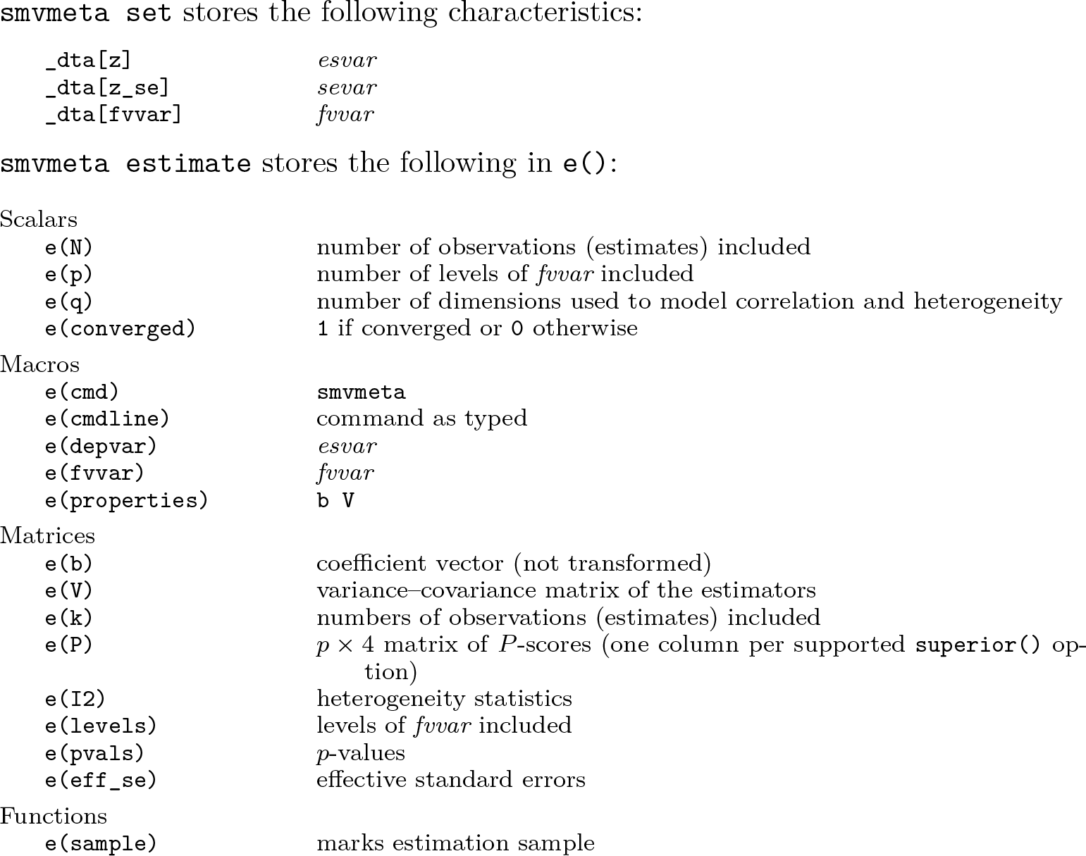
In addition to the above, the following are stored in

Note that results stored in
3 Example: Risk factors for pain after knee replacement
3.1 Background
The development of
The review identified and extracted estimates of association between risk factors measured at baseline prior to surgery and pain measured 12 months after surgery. Because it is generally not possible to randomize patients to risk factors, the review was based on observational studies. To facilitate meta-analysis of estimates of association reported using various metrics (for example, risk ratios, odds ratios, mean differences, and correlations) and between risk factors and pain assessments measured using a mix of binomial and continuous variables, correlation coefficients were extracted or imputed and then Fisher z-transformed. The following example is illustrative and may differ from the published systematic review.
3.2 Overview of pain12.dta
We begin by loading
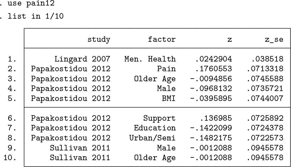
There are four variables with one effect-size estimate per row, as required by
Preprocessing would have been required had the data not been arranged in
3.3 Specify generic effect sizes, standard errors, and risk factors
The meta-analysis is specified using

Similarly to Stata’s
3.4 Meta-analysis using smvmeta estimate
Before running the meta-analysis, we first set the random-number generator’s seed to ensure that we can reproduce results and define a local macro,

We then use

The header section of the results table summarizes the analysis, providing information such as the number of observations (effect-size estimates) included in the analysis and the number of dimensions used to model correlation and heterogeneity. Each row of the table shows results for a particular risk factor. The first result is for Rey–Osterrieth complex figure (ROCF) recall, which assesses functional decline on multiple cognitive dimensions. Working left to right, the mean correlation between this variable and pain is estimated to be 0.342 with an effective standard error of 0.126 (section 4.3.3). The p-value testing the hypothesis that the mean correlation is zero is 0.005 (section 4.3.3). The 95% CI for mean correlation is [0.089 to 0.554] (section 4.3.3). Only one observation (study result) of correlation was used in the meta-analysis (column
In principle, we can now use almost all of Stata’s postestimation commands. For example, we could

This test gives a p-value of 0.045, suggesting that studies like those included in the metaanalysis generally estimate nonzero correlations between urban or semiurban residency and pain. However, the p-value provided by
3.5 Present estimates graphically using smvmeta forestplot
The command below uses


Forest plot showing estimates of mean correlation between risk factors and pain 12 months after total knee arthroplasty, the number of studies (k) contributing estimates, P-scores that measure the mean extent of certainty of superiority, and I2 values that measure the percentage of heterogeneity not explained by sampling error
The forest plot is shown in figure 2. The three risk factors estimated to have the greatest mean extent of certainty of superiority (that is, the highest P-scores; see section 4.4) are cognitive in nature: ROCF recall (see above; mean correlation 0.34; 95% CI [0.09 to 0.55]; P-score 92.4%). However, this finding is supported only by one study. Pain catastrophizing (0.28; 95% CI [0.12 to 0.42]; P-score 89%; 2 studies; I2 59.9%). Temporal summation, which—informally—assesses pain experienced with respect to the frequency of a controlled pain stimulus (0.21; 95% CI [0.05 to 0.36]; P-score 77.1%; 2 studies; I2 0.0%).
While it is useful to show estimates for all risk factors and all quantities that we can report, we might want to produce a simpler forest plot, for example, showing only a subset of the available columns, for “interesting” results. This can be done by specifying the forest plot columns of interest and an expression that restricts the results that should be presented (but does not change the estimates). We specify that we want to show columns for the names of the risk factors, the forest graph, effect-size point estimates (correlations, as transformed via the


A simplified presentation of the results, restricted to correlations with point estimates of at least 0.15 in magnitude and p-values less than 0.05
The forest plot is shown in figure 3. In addition to the three cognitive risk factors discussed above, the plot shows estimates for Kellgren–Lawrence grade (a tool for assessing radiological evidence of osteoarthritis) and number of symptomatic joints.
4 The estimator and its implementation
4.1 Assumptions and nomenclature
Let The n estimates of the p effect sizes are exchangeable across study. There are no nonrandom study-level effects. There is nonnegligible correlation and heterogeneity between effect sizes and studies that is well approximated in a low-dimensional space using a q × q covariance matrix No further information is available about the structure of the correlations and heterogeneity (for example, studies do not publish correlations between estimates).
Assumptions 1 and 2 explain why it is not necessary to specify to
4.2 Sparsity and smvmeta’s multivariate random-effects model
In the most general case, there may be correlation and heterogeneity between each pair of effect sizes. This gives p mean effect sizes, p(p − 1)/2 correlations, and p(p + 1)/2 covariances that model heterogeneity for a total of p+p2 model parameters. If p is even moderately large, then p + p2 is likely to be substantially larger than n, the number of estimates available to support estimation.
Assuming unstructured

A related dimensionality-reduction problem is principal component analysis (Pearson 1901; Jolliffe 2005). In principal component analysis, a linear transformation into a low-dimensional space can be defined via eigendecomposition of a known or estimated covariance matrix. A matrix of the eigenvectors with largest eigenvalues defines a transform that preserves at least a chosen proportion of total variation. This is possible if the covariance matrix is known or can be estimated but cannot be used to choose q because
The term “random projection” is typically used in the context of mapping point sets from high- to low-dimensional spaces in a way that approximately preserves some useful aspect of the data, particularly relative distances between points.
For some meta-analyses, it may be possible to use a priori domain knowledge to choose q. For example, perhaps it is reasonable to consider some effect sizes as facets of a common construct for which distinct estimates are desired, preventing pooling at the level of the construct, but facilitating dimensionality reduction. In general, however, domain knowledge may not be available to choose q. If q is not specified via the
4.3 Estimation
4.3.1 Penalized maximum likelihood
The primary estimation target is
The log density corresponding to

where
4.3.2 Optimization strategy
The optimization problem described above can be nontrivial. I found that Stata’s default optimization algorithm (modified Newton–Raphson) sometimes failed to converge and other algorithms often failed to start in a fruitful direction. Optimization is performed by initializing the elements of
Optimization can fail if q is too high.
4.3.3 Constructing CIs and p-values
We seek a test statistic and its sampling distribution to construct 100(1 − α)% CIs and p-values on the elements of effect-size vector
Cole, Chu, and Greenland (2014) provide a useful introduction to likelihood ratiobased CIs. Briefly, in the nonpenalized case, CIs can be constructed for βj (the jth effect size) on the basis that

where f is the log-likelihood function and
Let g and gj be log-penalty equivalents of f and fj. To account for penalization, we are interested in the distribution of
The sum of an arbitrary number of gamma variates has moment-generating function M(s) = s−1 ∏ i (1 − λis) −a , where a is a shape parameter common to the gamma variates and λi is the ith eigenvalue of a matrix constructed from the scale parameters and the correlation coefficients between the variates (Alouini, Abdi, and Kaveh 2001). In the case of the sum of two gamma variates with correlation ρ, this simplifies to

The inverse Laplace transform of (3) can be used to obtain the cumulative distribution function of Uj for a particular value of ρ and hence a sampling distribution that can be used to compute critical values and p-values.

Equation (4) can be used to test the hypothesis Hj : βj = 0. The test statistic is
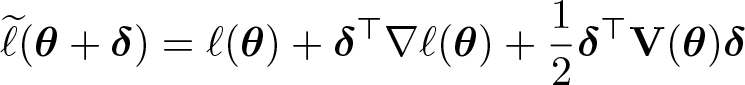
Having identified the distribution from which a critical value can be computed, we can find bounds βL and βU for βj efficiently via a quadratic approximation of ℓ around

where ℓ(
is used to find a value of

where η is a Lagrange multiplier and

Negative and positive values of η yield lower and upper bounds βL and βU, respectively. The quantities in (5) are iteratively updated, starting at

Constructing the test statistic, uj for Hj : βj = 0, and approximate CI bounds βL and βU for βj, via profile penalized likelihood
Recall that Wald-type CIs that are constructed from standard errors obtained from the variance–covariance matrix of the estimators do not necessarily have nominal coverage.
4.3.4 Alternative approaches to penalization
Penalized maximum likelihood is used by
The model used by
4.4 Assessing superiority
Multivariate meta-analyses are often motivated by a need to know which effect size is “superior” or to rank them. For example, it is natural to ask which risk factor is most important or which of several treatments is most effective.
4.4.1 Computing P-scores
The following presentation differs slightly from that of Rücker and Schwarzer (2015) but describes the method concisely in a way that is hopefully relatively intuitive. Assume momentarily that, of two effect sizes, the one closest to +∞ is superior. Let πi,j be a one-sided p-value for the null hypothesis βi ≤ βj. Then define the p × p matrix

The elements of this matrix are simply 1 minus the one-sided p-values, such that Pi,j will be close to unity if there is strong evidence that βi > βj.
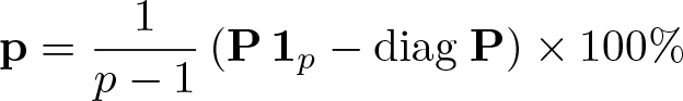
where
4.4.2 Defining superiority
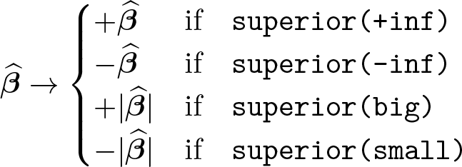
So far we have assumed that, of two effect sizes, the one closest to +∞ is superior. This corresponds to the
If relative risks less than unity were associated with the outcome, it may be useful to reverse the definition of superiority so that a P-score of 100% would have the interpretation of superiority rather than inferiority. Similarly, in meta-analyses of correlation coefficients, correlations with large magnitudes may be considered superior to small correlations. Section 2.2.2 describes four options for
4.4.3 Alternative methods for assessing superiority
P-scores and their Bayesian equivalent, surface under the cumulative ranking curve (SUCRA) values (Salanti, Ades, and Ioannidis 2011), have been argued to be preferable to the simpler approach of estimating a Bayesian posterior probability that a given effect size is superior to all others, for example, as implemented by the
A weakness of estimating posterior probabilities of superiority is that an imprecisely estimated effect size may have substantial probability mass for effect sizes that are implausibly large in magnitude. This phenomenon is most apparent in meta-analyses of correlations in which the magnitude of a coefficient, rather than its magnitude and direction, determines superiority. The probability mass in the tails of a posterior distribution that extends far in the negative and positive directions “doubles up” after taking the magnitude of the effect size. Consequently, the posterior probability that the effect size is indeed superior (or inferior) may also be large.
There is nothing wrong with such a probability: there really is a high posterior probability of superiority. 3 However, such a result can lack face validity and cause nonstatisticians to doubt the entire analysis. This is not unreasonable. Few people should accept that an imprecisely estimated quantity is highly likely to be superior to other quantities that are supported by much stronger evidence. P-scores and SUCRA values are quite robust to this problem but are admittedly more challenging to interpret.
An additional benefit of P-scores is that they are trivial to compute. In particular, it is not necessary to use sampling-based estimation methods, as is the case with SUCRA values and posterior probabilities of superiority. This means that results can be obtained quickly.
5 Simulation-based validation
I ran three simulation experiments to validate a prerelease version of
In the first two experiments, effect-size estimates were missing within each simulated study either completely at random (MCAR) or not at random (MNAR). The MNAR scenario used almost the same data as the MCAR scenario, but I discarded effect-size estimates—the values “published” by simulated studies—if their CIs included ±0.05. This models a publication bias scenario in which studies do not publish effect-size estimates if they are small or imprecisely estimated. I assumed no “domain knowledge” was available to choose q, the dimension in which correlation and heterogeneity are approximated. In these scenarios,
The third experiment was an MCAR scenario in which a priori estimates of q were assumed to be available. Values of q were obtained by applying principal components analysis to the known correlation matrices used to generate the simulated data. In each of these meta-analyses, I set
I generated synthetic data for 1,000 meta-analyses for each experiment. I used the known mean effect sizes to quantify and compare bias and empirical coverage of 95% CIs with results of random-effects meta-regressions in which mean effect size is estimated via a categorical covariate. This is a simple alternative model choice that can be applied to high-dimensional sparse data. It does not account for correlations between effect sizes and assumes heterogeneity is the same for all effect sizes.
Results for the three scenarios were very similar, suggesting that
These findings are perhaps unsurprising given that random projection works less well in lower dimensions and that it will not always be possible to model correlation and heterogeneity between many effect sizes in a low-dimensional space. The experiments suggest that
In the third experiment, the prespecified value of q was used in about 87% of metaanalyses. Around 10% of meta-analyses used a value of q 1 less than the prespecified value. The median number of dimensions used was six. Fewer than 1% of analyses used a value of q less than 4, and fewer than 1% used a value greater than 7. These findings suggest that 4 ≤ q ≤ 7 is probably reasonable if you want to specify q and the number of effect sizes is not more than 30, but
6 Conclusions
This article has presented
The command was demonstrated in an example multivariate meta-analysis of pain after total knee arthroplasty. Mathematical and computational details of the model and P-scores were then presented. Simulation-based validation experiments show that, in the higher-dimensional sparse setting for which
The fundamental limitations of
8 Programs and supplemental materials
Supplemental Material, sj-zip-1-stj-10.1177_1536867X241258008 - Multivariate random-effects meta-analysis for sparse data using smvmeta
Supplemental Material, sj-zip-1-stj-10.1177_1536867X241258008 for Multivariate random-effects meta-analysis for sparse data using smvmeta by Christopher James Rose in The Stata Journal
Footnotes
7 Acknowledgments
The author thanks Unni Olsen, Maren Falch Lindberg, and Anners Lerdal (University of Oslo and Lovisenberg Diaconal Hospital, Norway), Eva Marie-Louise Denison (Norwegian Institute of Public Health), and Arild Aamodt (Lovisenberg Diaconal Hospital) for their work on the systematic reviews that motivated development of
8 Programs and supplemental materials
To install a snapshot of the corresponding software files as they existed at the time of publication of this article, type
Notes
References
Supplementary Material
Please find the following supplemental material available below.
For Open Access articles published under a Creative Commons License, all supplemental material carries the same license as the article it is associated with.
For non-Open Access articles published, all supplemental material carries a non-exclusive license, and permission requests for re-use of supplemental material or any part of supplemental material shall be sent directly to the copyright owner as specified in the copyright notice associated with the article.