Sage Journals: Discover world-class research

Abstract

In this article, we describe the mixrandregret command, which extends the randregret command introduced in Gutiérrez-Vargas, Meulders, and Vandebroek (2021, Stata Journal 21: 626–658) by allowing random coefficients in random regret minimization models. The newly developed mixrandregret command allows the user to specify a combination of fixed and random coefficients in the regret function of the classical random regret minimization model introduced in Chorus (2010, European Journal of Transport and Infrastructure Research 10: 181–196). In addition, the user can specify normal and lognormal distributions for the random coefficients using the appropriate command’s options. The models are fit by maximum simulated likelihood estimation using numerical integration to approximate the choice probabilities.

Keywords

st0746 mixrandregret mixrpred mixrbeta discrete choice models random regret model logit model random coefficients

1 Introduction

McFadden (1974) introduced the conditional logit model to explain individuals’ choice behaviors and to predict market shares of products and services. The conditional logit model forms the basis for most discrete choice models, which assume that individuals use a decision rule based on random utility maximization (RUM) when choosing among alternatives. In contrast, Chorus, Arentze, and Timmermans (2008) proposed an alternative decision rule known as random regret minimization (RRM), which assumes that decision makers aim to minimize regret when making their choices. McFadden and Train (2000) extended the random utility model by allowing the parameters to vary across individuals, leading to the so-called mixed logit model. Similarly, Hensher, Greene, and Ho (2016) extended the RRM models to include random effects, which account for preference heterogeneity and allow for correlation among choices made by the same individual. This article introduces the mixrandregret command, which allows users to fit this mixed version of the RRM models.

There is a growing literature on empirical applications of RRM to various topics, including wildfire evacuation (Wong et al. 2020), students’ travel patterns (Anowar et al. 2019), healthcare choices (Boeri et al. 2013), and consumer choices (Chorus, Koetse, and Hoen 2013). Unfortunately, there is no clear guidance on how to choose between an RRM and a RUM model, and selecting the decision rule is, indeed, still an open question within the discrete choice literature. In practice, the decision rule is often selected using information criteria or the models’ predictive power, depending on the research objectives. Some researchers even tried to combine different decision rules into one model (Hess, Stathopoulos, and Daly 2012; Lim and Hahn 2020), which is a very promising research avenue and also one of the potential extensions of our own mixrandregret command (see section 7).

One article that provides theoretical guidance on the effects of regret in the context of consumer psychology is Pieters and Zeelenberg (2007). The authors argue that regret becomes more relevant when consumers find the decision complex, important, or significant to themselves or their peers. Hence, the relevance of the regret is tied to the individuals’ perception of the choices they are making. Additionally, the empirical application of Lim and Hahn (2020) using regulatory focus theory (Higgins 1997, 1998) surveyed the individuals and gave them scores using the chronic regulatory focus index (CRFI), which is a continuous index that has two opposite profiles. On one hand, negative CRFI values are associated with “prevention-focused” consumers who value safety and security and are concerned about potential losses. On the other hand, positive CRFI values are associated with “promotion-focused” consumers who value the existence of positive outcomes and emphasize the rewards, focusing on the potential gains. Using the CRFI, Lim and Hahn (2020) found that “prevention-focused” consumers tended to behave more as regret minimizers and “promotion-focused” individuals tended to behave as utility maximizers. Hence, the individuals’ characteristics might also affect the intensity of the regret they are experiencing.

As mentioned, determining an individual’s decision rule is still an open question and, as of now, is generally selected by examining the model fit. However, regret-based models have additional behavioral components compared with their utility counterparts. For instance, regret-based models exhibit so-called semicompensatory behavior, meaning that the regret experienced by a given difference in attribute levels has more weight than the rejoicing obtained from the same attribute-level difference when comparing the alternatives in the choice set. As a consequence of the semicompensatory behavior of the regret models, the so-called compromise effect (Chorus and Bierlaire 2013) can be observed. Consequently, alternatives with more balanced overall performances across attributes are preferred to high-performing alternatives with potentially only one severely underperforming attribute. This is due to the semicompensatory behavior, by which the regret derived from this poorly performing attribute is not entirely compensated by the rejoicing of the high-performing ones. A detailed description of this behavior and a comparison of the semicompensatory behavior among different regret functions can be found in Gutiérrez-Vargas, Meulders, and Vandebroek (2021)

Both the RRM and the RUM models can be extended by allowing random coefficients to model heterogeneous preferences in the population. By doing so, we can model that not all individuals experience the same magnitude of regret (or utility) for a given attribute. We can estimate the distribution of the population’s regret coefficients, and afterward, using postestimation procedures, we can compute the individual-level regret parameters. This extension of the model results in so-called unobserved preference heterogeneity, where a parametric distribution captures the differences in taste across individuals that are beyond what we can do using the information on the sample (that is, interaction terms with individual characteristics). We refer to this random-coefficient regret model as the mixed RRM model. The mixed RRM has been used by Boeri and Masiero (2014) and Hensher, Greene, and Ho (2016) in the past using transport data. In both articles, the authors find that the mixed RRM has a slightly better model performance than mixed RUM models, which is not to say that this will always be the case, but it does show that in some contexts, regret-based models might outperform their utility-based models and that it is worth investigating them, especially if the modeler considers that the conditions presented in Pieters and Zeelenberg (2007) for a strong regret effect to hold are applicable.

The rest of the article is organized as follows. In section 2, we briefly introduce the classic RRM model, some of its properties, and its corresponding likelihood function. Section 3 introduces the mixed RRM model, which extends the classic RRM model by allowing for random coefficients. This section also comments on how the formulas presented in section 2 are updated to allow the inclusion of random parameters. It also presents the likelihood function of the mixed RRM model and introduces the maximum simulated likelihood estimation procedure that we use to maximize it. Section 4 describes the estimation of individual-level parameters after the estimation of the mixed RRM model, allowing us to find the regret-specific parameters for each individual in the sample. Section 5 describes the syntax of every command included in our package. Section 6 provides a comprehensive example of the usage of the package using discrete choice data from van Cranenburgh (2018), showing how to fit a mixed RRM model using the mixrandregret command and how to compute the individual-level parameters using the mixrbeta command. Additionally, it shows how to compute predicted probabilities with the mixrpred command. Finally, section 7 concludes and lists some potential improvements and extensions.

2 Classical random regret models

On one hand, RUM models assume that individuals are utility maximizers when selecting an alternative from a discrete set of alternatives. On the other hand, RRM models assume that individuals are regret minimizers. Regret occurs when, compared with other available alternatives, the selected alternative is outperformed by the other alternatives in some attributes (Loomes and Sugden 1982). RRM models assume that individuals will choose the alternative that minimizes the random regret resulting from comparing their relative performance with the other nonchosen alternatives in the choice set. Formally, Chorus, Arentze, and Timmermans (2008) presented an initial model for RRM models, and Chorus (2010) modified the regret function to obtain a smooth likelihood function. Accordingly, he proposed the model in (1) to denote the regret of an individual n when choosing alternative i of the J possible alternatives.

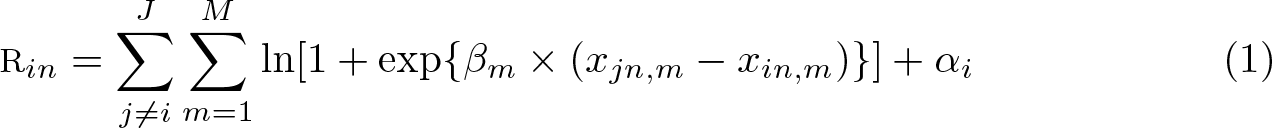
R_{i n} = \sum_{j \neq i}^{J} \sum_{m = 1}^{M} \ln [1 + \exp {β_{m} \times (x_{j n, m} - x_{i n, m})}] + α_{i}

More specifically, (1) represents the regret that an individual (referred to by n) experiences when choosing alternative i out of J alternatives (referred to by j or i). Additionally, each alternative is described in terms of the value of M attributes (referred to by m). Consequently, x_in,m represents the values of attribute m of alternative i for individual n, and β_m is the taste parameter of attribute m that is shared by every individual n. The parameter β_m indicates that with each unit increase in the difference between the attribute level of alternative i and the rest of the alternatives, regret would either increase (if β_m is positive) or decrease (if β_m is negative). Besides, we can include alternative specific constants (ASC) by simply adding them to the systematic part of the regret. The inclusion of the ASC serves the same purpose as in RUM models: to account for omitted attributes for a particular alternative i. As usual, for identification purposes, we need to exclude one of the ASC from the model specification, so we define α = (α_i,…, α_J−₁) as the vector of J − 1 ASC included in the model. For a detailed discussion of the ASC in the context of RRM models, check van Cranenburgh and Prato (2016). Consequently, R _in describes the total systematic regret for an individual n choosing alternative i.

As with RUM models, we can obtain the random regret function, RR _in , by adding an independent and identically distributed extreme-value type I error term to the systematic regret function R _in to account for pure random noise and the impact of omitted attributes on the regret function: RR _in = R _in + ε_in. Mathematically, the minimization of the random regret function is equivalent to maximizing the negative function, which results in the conventional closed-form logit formula for the choice probabilities given in (2).

P_{i n} = \frac{\exp (- R_{i n})}{\sum_{j = 1}^{J} \exp (- R_{j n})}

The log-likelihood (LL) function of the regret model for N individuals is given by (3), where β = (β₁,…, β_m) is the vector of taste parameters and y_in is the dummy variable that takes the value of 1 when alternative i is chosen by individual n and 0 otherwise.

LL (α, β) = \sum_{n = 1}^{N} \sum_{i = 1}^{J} y_{i n} \times \ln (P_{i n})

In the literature, there are several extensions of the classical RRM models. For instance, Chorus (2014) proposed the generalized RRM, which replaces the “1” in the regret function with a new parameter, γ_m, denoting the regret weight for attribute m. Additionally, van Cranenburgh, Guevara, and Chorus (2015) incorporated a scale parameter into the RRM, which is now referred to as µRRM. The pure RRM was proposed in the same article (van Cranenburgh, Guevara, and Chorus 2015) as a special case of µRRM when µ is arbitrarily small. For a review that compares the different types of RRM models and RUM models, see Gutiérrez-Vargas, Meulders, and Vandebroek (2021). In what follows, we will focus on the classical regret function of Chorus (2010) as described in (1) and allow for random taste parameters as introduced by Hensher, Greene, and Ho (2016). This model will be referred to as the mixed RRM model, which assumes a parametric distribution for the taste parameters.

3 Mixed RRM models

In this section, we describe the mixed RRM model, which has two major differences with respect to the classic RRM model. First, it includes random coefficients that follow a parametric distribution to model taste heterogeneity. Second, as we will explain in this section, the model can accommodate the presence of panel structure in the data. Introducing the parametric distribution for the taste parameters triggers a new subindex to the taste parameters vector, β _n = (β_n,₁,…, β_n,m), which now follows a parametric distribution f( β|φ ), where φ are the parameters that describe the distribution.¹ Hence, β_n,m is now an individual-specific taste parameter that represents the regret sensitivity of individual n to changes in attribute m. Additionally, when multiple choice situations (referred to by s) are answered by the same individual, we are in the presence of a paneldata structure, which triggers the inclusion of a new subindex for the choice situations in our formulas. Hence, x_ins,m will now represent the value of attribute m in alternative i for individual n in choice situation s. Similarly, y_ins is now a binary variable that takes the value of 1 when individual n chooses alternative i in choice situation s and 0 otherwise. That being said, we will define the new regret function in (4), where R _ins describes the systematic regret for individual n choosing alternative i in choice situation s.

R_{i n s} = \sum_{j \neq i}^{J} \sum_{m = 1}^{M} \ln [1 + \exp {β_{n, m} \times (x_{j n s, m} - x_{i n s, m})}] + α_{i}

Similarly, as in the classical RRM model, we add an independent and identically distributed extreme value type I error term to the systematic regret function, and we obtain the choice probabilities given by (5).

P_{i n s} = \frac{\exp (- R_{i n s})}{\sum_{j = 1}^{J} \exp (- R_{j n s})}

The probability of the entire sequence of observed choices of individual n (conditional on knowing β _n ) is given by (6), which replaces (2) in the classic RRM model. By doing so, the model considers each individual’s sequence of choices as independent blocks of observations, contrary to the classic model, which assumes that every choice set is independent (regardless of the individual who answered it).

P_{n} (α, β) = \prod_{s = 1}^{S} \prod_{j = 1}^{J} {(P_{i n s})}^{y_{i n s}}

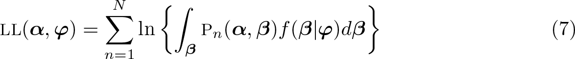
The unconditional choice probabilities of the observed sequence of choices are the conditional choice probabilities [see (6)] integrated over the entire domain of the distribution. Consequently, the LL function of the mixed RRM model is in (7).

L L (α, φ) = \sum_{n = 1}^{N} \ln {\int_{β} P_{n} (α, β) f (β ∣ φ) d β}

Given that the integral described in (7) does not have a closed-form solution, it is approximated using simulation (Train 2009). Accordingly, we fit the model by maximum simulated likelihood. We approximate the LL function by (8), where R is the number of draws and β ^r is the rth draw from f( β |φ). We use Halton draws to create the draws used to approximate the choice probabilities. We maximize this simulated log-likelihood (SLL) function to obtain estimates for the parameters α and φ .

SLL (α, φ) = \sum_{n = 1}^{N} \ln {\frac{1}{R} \sum_{r = 1}^{R} P_{n} (α, β^{r})}

4 Individual-level parameters

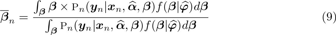
After maximizing the SLL function to obtain estimates for $\hat{φ}$ and $\hat{α}$ , we can compute estimates for the individual-level parameters. This is conditional on their sequences of choices (denoted by y _n ) and given the attribute levels for every alternative and choice set, denoted by x _n , that the individual faced when making the choices. For instance, we can compute the individual-level parameter ${\bar{β}}_{n}$ for an individual n, which corresponds to the mean of the distribution of β _n conditional on y _n , x _n , and our estimated $\hat{φ}$ and $\hat{α}$ . The expression for ${\bar{β}}_{n}$ is given in (9), and its derivation can be found in Train (2009):

{\bar{β}}_{n} = \frac{\int_{β} β \times P_{n} (y_{n} ∣ x_{n}, \hat{α}, β) f (β ∣ \hat{φ}) d β}{\int_{β} P_{n} (y_{n} ∣ x_{n}, \hat{α}, β) f (β ∣ \hat{φ}) d β}

Again, because there is no closed-form solution for the integrals in (9), we approximate them using simulations yielding (10),

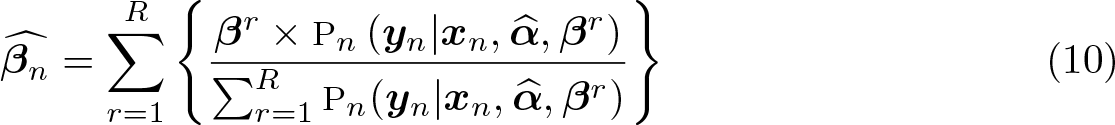
\hat{β_{n}} = \sum_{r = 1}^{R} {\frac{β^{r} \times P_{n} (y_{n} ∣ x_{n}, \hat{α}, β^{r})}{\sum_{r = 1}^{R} P_{n} (y_{n} ∣ x_{n}, \hat{α}, β^{r})}}

R is the number of draws, and β ^r is the rth draw from f( β | φ ).

5 Commands

5.1 mixrandregret

Syntax

depvar equal to 1 identifies the chosen alternative, whereas depvar equal to 0 indicates that the alternative was not selected. There is only one chosen alternative for each choice set. fweights, iweights, and pweights are allowed (see [U] 11.1.6 weight), but they are applied to decision-makers, not to individual observations.

Description

Mixrandregret fits the mixed RRM model described in Hensher, Greene, and Ho (2016), a mixed version of the classic RRM model introduced in Chorus (2010). mixrandregret extends the randregret command (Gutiérrez-Vargas, Meulders, and Vandebroek 2021) and allows the user to specify normally and lognormally distributed taste parameters inside the regret function. The command uses maximum simulated likelihood for estimation (Train 2009).

Options

id(varname) is required and specifies a numeric identifier variable for the decisionmakers.

group(varname) is required and specifies a numeric identifier variable for the choice situations.

rand(varlist) is required and specifies the independent variables whose coefficients are random. The random coefficients can be specified to be normally or lognormally distributed (see the ln() option). The variables immediately following the dependent variable in the syntax have fixed coefficients.

alternatives(varname) is required to identify the alternatives available for choice situations.

basealternative(#) sets the base alternative for defining the ASC if they are not suppressed.

noconstant suppresses the ASC.

cluster(varname), robust; see [R] vce_option . The cluster variable must be numeric.

ln(#) specifies that the last # variables in rand() have lognormally rather than normally distributed coefficients. The default is ln(0).

nrep(#) specifies the number of Halton draws used for the simulation. The default is nrep(50).

burn(#) specifies the number of initial elements to be dropped when creating the Halton sequences. The default is burn(15). Specifying this option helps reduce the correlation between the sequences in each dimension.

level(#) sets the confidence level. The default is level(95).

maximize_options are difficult, technique(algorithm_spec), iterate(#), trace, gradient, showstep, hessian, tolerance(#), ltolerance(#), gtolerance(#), nrtolerance(#), from(init_specs); see [R] Maximize.

5.2 mixrpred

Syntax

Description

Following mixrandregret, mixrpred can be used to obtain the predicted probabilities.

Options

proba calculates the choice probability for each alternative for each choice situation; this is the default option.

nrep(#) specifies the number of Halton draws used for the simulation. The default is nrep(50).

5.3 mixrbeta

Syntax

Description

mixrbeta can be used after mixrandregret to calculate individual-level parameters for all the variables in the specified varname using (10). The individual-level parameters are stored in a user-specified data file.

Options

saving(filename) saves individual-level parameters to filename. saving() is required.

plot plots the distributions of the individual-level parameters.

nrep(#) specifies the number of Halton draws used for the simulation. The default is nrep(50).

burn(#) specifies the number of initial sequence elements to be dropped when creating the Halton sequences. The default is burn(15). Specifying this option helps reduce the correlation between the sequences in each dimension.

replace overwrites filename.

6 Examples

To show how we can fit mixed RRM models using the mixrandregret command, we use data from a stated choice experiment that was utilized in van Cranenburgh, Rose, and Chorus (2018). The participants answered 10 choice situations where they chose from 3 unlabeled route alternatives with 2 attributes: travel cost and travel time. The following variables are used in our illustration:

altern: the alternative faced by the user (subindex i or j).

choice: whether the alternative was chosen by the individual (dummy, 1 if chosen).

id: ID of the individual.

cs: ID of the choice situation faced by the individual.

tt: total travel time of the alternative in minutes.

tc: total travel cost of the alternative in euros.

We follow the data setup in randregret (see Gutiérrez-Vargas, Meulders, and Vandebroek [2021]), and the setup for mixrandregret is also identical to that required by mixlogit (see Hole [2007]), which is the panel representation in long format where each row represents an alternative for a given choice set. The dataset can be downloaded directly from van Cranenburgh (2018) and then loaded in Stata. We keep the variables of interest and list the first three observations. As can be seen below, the data loaded are in wide format because each row corresponds to a choice situation.

Following the data manipulation in Gutiérrez-Vargas, Meulders, and Vandebroek (2021), we transform the dataset using the reshape command and present the data in the required long format below. We list the first 12 rows, and each row now corresponds to an alternative. The dependent variable choice is 1 for the chosen alternative in each choice situation and 0 otherwise. altern identifies the alternatives in a choice situation, cs identifies the choice situation faced by the individual, and id identifies the individual. Furthermore, total_time and total_cost are obtained from the tt and tc variables.

We begin by fitting a classical RRM model using the randregret command to obtain reasonable starting values for mixrandregret. We also declare noconstant, suppressing the ASC given that alternatives are nonlabeled in the survey. If we have labeled data, we can specify the base alternative by declaring the base() option. Because we have repeated choices from a given individual, the standard errors are corrected by specifying cluster(id).

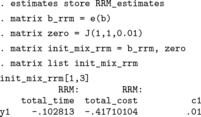
As expected, both parameter estimates are negative and highly significant, suggesting that regret decreases as the level of travel time or travel cost increases in a nonchosen alternative compared with the same attribute level in the chosen one. The coefficients are saved in init_mix_rrm for later use as initial values for mixrandregret.

We then fit a mixed RRM model in which we let the coefficient for total_cost be nonrandom, but we specify the coefficient for total_time as normally distributed. We use the option from() in mixrandregret to initialize the optimization routine using the values saved in init_mix_rrm as the starting point for the mean for the total_time parameter. We fit the model using 500 Halton draws to approximate the choice probabilities as in (8). We also clustered the standard errors at the individual level using cluster(id).

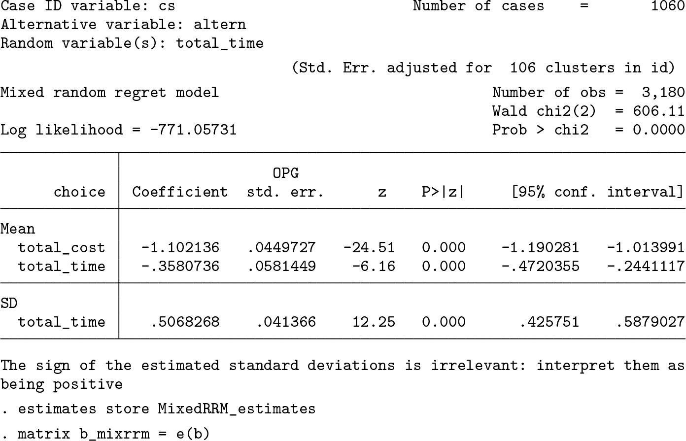
On average, the regret decreases as the total travel time increases in a nonchosen alternative, compared with the same level of travel time in the chosen alternative. The interpretation is similar for the total travel cost attribute. Additionally, we observe that the estimated standard deviation for the normal distribution of total travel time is significantly different from zero, which implies the existence of heterogeneity in the sample.

We can also perform a likelihood-ratio test to see whether the mixed RRM fits the data better than the previously fitted classical RRM model. It is crucial to notice that a standard deviation cannot be negative, and that by testing whether the standard deviation parameter is larger than zero, we are performing a statistical test with a null hypothesis in which the parameter is on the boundary of its parametric space. This is a well-studied problem in the literature of generalized linear mixed models (Verbeke and Molenberghs 2000), and we have to correct the distribution for the statistic under the null hypothesis using a mixture of χ² distributions in which 50% of the probability mass is at 0 and the other 50% uses the conventionally used (uncorrected) χ² distribution. This correction implies we must halve the p-values found using the uncorrected distribution. Notably, the correction described here is valid only when testing the inclusion of one extra random coefficient to the utility specification. However, details for the corrections needed when including more than one random coefficient can be found in Stram and Lee (1994) and Verbeke and Molenberghs (2000, sec. 6.3.4). Looking at the results of the likelihood-ratio test, we can see that we reject the null hypothesis even when halving the p-value.² Hence, the mixed RRM model does fit the data better than the classic RRM model. As an alternative heuristic procedure, Hensher and Greene (2003) suggested using a model with all attributes included as random and then inspecting whether the standard deviation parameters of the random coefficients are different from zero using t-test statistics.

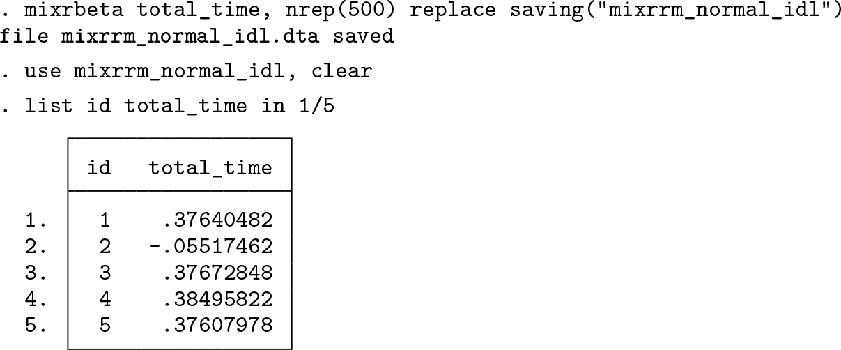
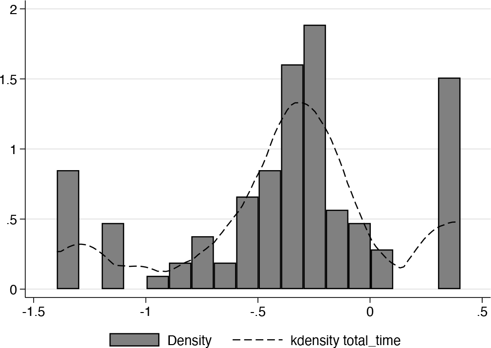
After fitting the mixed RRM model, we can compute individual-level parameters using mixrbeta. In the code below, we use (10) to approximate the value for the regret coefficient for each individual using 500 Halton draws. mixrbeta creates a new dataset with one observation per individual (id) and its corresponding parameter estimates. We display the estimates for the first five individuals in the sample, where we observe that some of them have a positive coefficient for the total_time attribute. Besides, we plot the individual-level parameters for total_time in figure 1 for all the individuals in the sample and observe that there are individuals with positive estimates for the total_time coefficient, which is counterintuitive.

Figure 1.

Distribution of total time coefficient (normal)

One solution to obtain nonpositive estimates for the total_time coefficient is to use a bounded distribution. For this purpose, when using mixrandregret, we can specify that a coefficient is lognormally distributed. In our case, because we want a nonpositive distribution for the total_time coefficient, we have to multiply the total_time attribute by −1 to ensure that it is nonpositive. To this end, we create the new variable ntt, which corresponds to the negative of total_time.

The estimated parameters correspond to the mean ntt and the standard deviation of the natural logarithm of the coefficient, and we can transform them back to the estimates of the coefficients themselves. The median of the coefficient is given by exp(b_ntt), the mean is given by $\exp (b_{ntt} + s_{ntt}^{2} / 2)$ , and the standard deviation is given by $\exp (b_{ntt} + s_{ntt}^{2} / 2)$ × $\sqrt{\exp (s_{ntt}^{2}) - 1}$ (Train 2009). The sign change prior to the estimation is reversed by multiplying the estimates by −1.

Again, we calculate individual-level parameters. As we can observe in the listed data and distribution presented in figure 2, all individual-level parameters are now negative as we expected.

Figure 2.

Distribution of total time coefficient (lognormal)

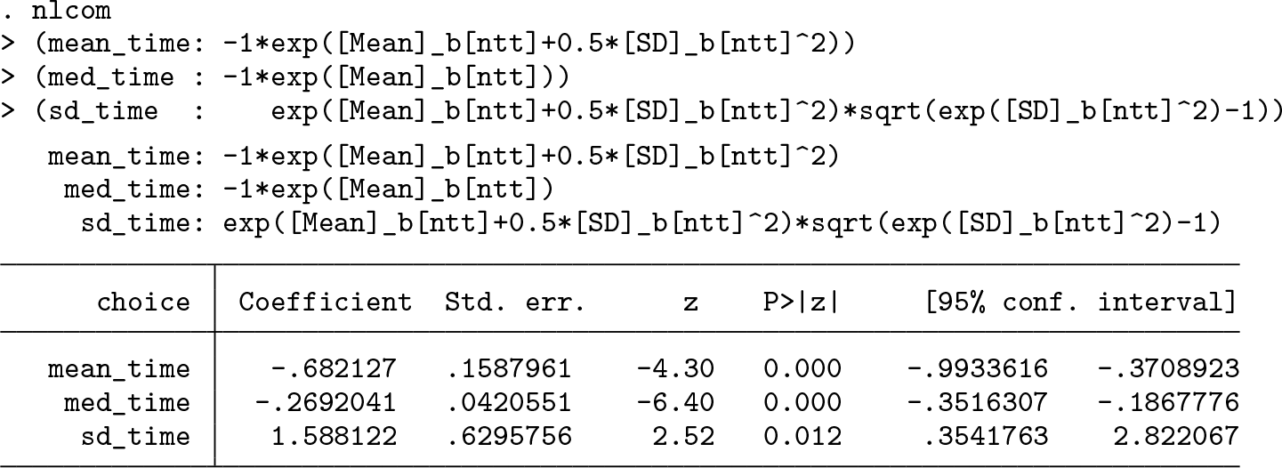
After running mixrandregret, we can also generate predictions using mixrpred. Using the option proba, we generate the pred_p_ln variable containing the predicted probability for each alternative. The code and output are listed below.

Additionally, mixrandregret allows for the inclusion of ASC if users have labeled data. Although the dataset is unlabeled in this example, we treat it as a labeled one assuming that each alternative represents a distinct category. We run the model including the basealternative(1) option, which specifies that the first alternative is the reference group for ASC.

7 Conclusions

This article presented the mixrandregret command to fit RRM models with random parameters. We showed how to use two postestimation commands. First, we used mixrpred to compute each alternative’s predicted probability. Second, we illustrated the use of mixrbeta to estimate individual-level parameters for the random coefficients. The commands’ usage and options are illustrated using discrete choice data from van Cranenburgh (2018).

The package we presented in this article still has room for improvement, and the most critical current deficiency is its speed. Given that the model has to compute attribute-level differences, the computation time also increases considerably when the size of the choice set increases. One possible solution to this issue is to use Stata’s C++ plugin, which compiles a portion of the code in the C++ programming language and loads the results into Stata. Several extensions can be implemented to the presented package. First, the package can be extended by implementing mixed versions of the generalizations of the RRM models, namely, the γRRM (Chorus 2014), the µRRM, and the pure RRM models (van Cranenburgh, Guevara, and Chorus 2015). Besides, the package could include more distributions for the random coefficients, such as uniform, triangular, or restricted normals. Another avenue for further extending the command is to combine regret-based models with latent class (LC) models (Bhat 1997). LC models assume that there are several LCs present in the data and each class has different taste coefficients. Utility-based LC models are readily available in Stata using the commands lclogit (Pacifico and Yoo 2013) and lclogit2 (Yoo 2020). One extension might be to develop a package that can fit an LC model in which some LCs follow RUM while other classes follow RRM decision rules as was done in Hess, Stathopoulos, and Daly (2012). Even further, the LC model could be extended into an LC model with random coefficients, allowing some taste parameters to follow a given distribution inside each class. Using the LC allocation model, we can also use individuals’ characteristics to allocate individuals into different classes with different decision rules. This can also provide further insights into which kinds of individuals might be performing regret-based decisions instead of utility-based decisions.

12 Programs and supplemental material

Supplemental Material, sj-zip-1-stj-10.1177_1536867X241257802 - Fitting mixed random regret minimization models using maximum simulated likelihood

Supplemental Material, sj-zip-1-stj-10.1177_1536867X241257802 for Fitting mixed random regret minimization models using maximum simulated likelihood by Ziyue Zhu, Álvaro A. Gutiérrez-Vargas and Martina Vandebroek in The Stata Journal

Footnotes

8 Acknowledgments

We thank Michel Meulders, Jan De Spiegeleer, and the participants from the 2022 London Stata Conference for their helpful comments and constructive suggestions. Additionally, substantial portions of our programs were inspired by the book Maximum Likelihood Estimation with Stata, Fifth Edition by Jeffrey Pitblado, Brian Poi, and William Gould (2024). Finally, many of the previous checks to the data and the construction of the LL functions were greatly inspired by the randregret (Gutiérrez-Vargas, Meulders, and Vandebroek 2021) and mixlogit () commands.

9 Funding

This work was produced while Álvaro A. Gutiérrez-Vargas was a PhD student at the Research Centre for Operations Research and Statistics at KU Leuven, funded by Bijzonder Onderzoeksfonds KU Leuven (Special Research Fund KU Leuven).

10 Conflict of interest

Ziyue Zhu, Álvaro A. Gutiérrez-Vargas, and Martina Vandebroek declare no conflicts of interest.

11 Contribution

Ziyue Zhu and Álvaro A. Gutiérrez-Vargas contributed equally to the article by developing the command and drafting the article. Martina Vandebroek critically commented on both the article and the command’s functionality.

12 Programs and supplemental material

To install the software files as they existed at the time of publication of this article, type

Notes

References

Anowar

Faghih-Imani

Miller

E. J.

Eluru

2019. Regret minimization based joint econometric model of mode choice and departure time: A case study of university students in Toronto, Canada. Transportmetrica A: Transport Science 15: 1214–1246. https://doi.org/10.1080/23249935.2019.1573859.

Bhat

C. R.

1997. An endogenous segmentation mode choice model with an application to intercity travel. Transportation Science 31: 34–48. https://doi.org/10.1287/trsc.31.1.34.

Boeri

Longo

Grisolía

J. M.

Hutchinson

W. G.

Kee

2013. The role of regret minimisation in lifestyle choices affecting the risk of coronary heart disease. Journal of Health Economics 32: 253–260. https://doi.org/10.1016/j.jhealeco.2012.10.007.

Boeri

Masiero

2014. Regret minimisation and utility maximisation in a freight transport context. Transportmetrica A: Transport Science 10: 548–560. https://doi.org/10.1080/23249935.2013.809818.

Chorus

C. G.

2010. A new model of random regret minimization. European Journal of Transport and Infrastructure Research 10: 181–196. https://doi.org/10.18757/ejtir.2010.10.2.2881.

Chorus

C. G.

2014. A generalized random regret minimization model. Transportation Research, B part 68: 224–238. https://doi.org/10.1016/j.trb.2014.06.009.

Chorus

C. G.

Arentze

T. A.

Timmermans

H. J. P.

2008. A random regretminimization model of travel choice. Transportation Research, B part 42: 1–18. https://doi.org/10.1016/j.trb.2007.05.004.

Chorus

C. G.

Bierlaire

2013. An empirical comparison of travel choice models that capture preferences for compromise alternatives. Transportation 40: 549–562. https://doi.org/10.1007/s11116-012-9444-3.

Chorus

C. G.

Koetse

M. J.

Hoen

2013. Consumer preferences for alternative fuel vehicles: Comparing a utility maximization and a regret minimization model. Energy Policy 61: 901–908. https://doi.org/10.1016/j.enpol.2013.06.064.

10.

Gutiérrez-Vargas

Á. A.

Meulders

Vandebroek

2021. randregret: A command for fitting random regret minimization models using Stata. Stata Journal 21: 626–658. https://doi.org/10.1177/1536867X211045538.

11.

Hensher

D. A.

Greene

W. H.

2003. The mixed logit model: The state of practice. Transportation 30: 133–176. https://doi.org/10.1023/A:1022558715350.

12.

Hensher

D. A.

Greene

W. H.

C. Q.

2016. Random regret minimization and random utility maximization in the presence of preference heterogeneity: An empirical contrast. Journal of Transportation Engineering 142: Article 04016009. https://doi.org/10.1061/(ASCE)TE.1943-5436.0000827.

13.

Hess

Stathopoulos

Daly

2012. Allowing for heterogeneous decision rules in discrete choice models: An approach and four case studies. Transportation 39: 565–591. https://doi.org/10.1007/s11116-011-9365-6.

14.

Higgins

E. T.

1997. Beyond pleasure and pain. American Psychologist 52: 1280–1300. https://doi.org/10.1037/0003-066X.52.12.1280.

15.

Higgins

E. T.

1998. Promotion and prevention: Regulatory focus as a motivational principle. In Vol. 30 of Advances in Experimental Social Psychology, ed. Zanna

M. P.

, 1–46. Academic Press. https://doi.org/10.1016/S0065-2601(08)60381-0.

16.

Hole

A. R.

2007. Fitting mixed logit models by using maximum simulated likelihood. Stata Journal 7: 388–401. https://doi.org/10.1177/1536867X0700700306.

17.

Lim

Hahn

2020. Regulatory focus and decision rules: Are preventionfocused consumers regret minimizers? Journal of Business Research 120: 343–350. https://doi.org/10.1016/j.jbusres.2019.11.066.

18.

Loomes

Sugden

1982. Regret theory: An alternative theory of rational choice under uncertainty. Economic Journal 92: 805–824. https://doi.org/10.2307/2232669.

19.

McFadden

1974. Conditional logit analysis of qualitative choice behavior. In Frontiers in Econometrics, ed. Zarembka

, 105–142. New York: Academic Press.

20.

McFadden

Train

2000. Mixed MNL models for discrete response. Journal of Applied Econometrics 15: 447–470. https://doi.org/10.1002/1099-1255(200009/10)15:5%3C447::AID-JAE570%3E3.0.CO;2-1.

21.

Pacifico

Yoo

H. I.

2013. lclogit: A Stata command for fitting latent-class conditional logit models via the expectation-maximization algorithm. Stata Journal 13: 625–639. https://doi.org/10.1177/1536867X1301300312.

22.

Pieters

Zeelenberg

2007. A theory of regret regulation 1.1. Journal of Consumer Psychology 17: 29–35. https://doi.org/10.1207/s15327663jcp1701_6.

23.

Pitblado

Poi

Gould

2024. Maximum Likelihood Estimation with Stata. 5th ed. College Station, TX: Stata Press.

24.

Stram

D. O.

Lee

J. W.

1994. Variance components testing in the longitudinal mixed-effects model. Biometrics 50: 1171–1177. https://doi.org/10.2307/2533455.

25.

Train

K. E

2009. Discrete Choice Methods with Simulation. 2nd ed. Cambridge: Cambridge University Press. https://doi.org/10.1017/CBO9780511805271.

26.

van Cranenburgh

2018. Small value-of-time experiment, Netherlands. 4TU.Centre for Research Data, Dataset. https://doi.org/10.4121/uuid:1ccca375-68ca-4cb6-8fc0-926712f50404.

27.

van Cranenburgh

Guevara

C. A.

Chorus

C. G.

2015. New insights on random regret minimization models. Transportation Research, A part 74: 91–109. https://doi.org/10.1016/j.tra.2015.01.008.

28.

van Cranenburgh

Prato

C. G.

2016. On the robustness of random regret minimization modelling outcomes towards omitted attributes. Journal of Choice Modelling 18: 51–70. https://doi.org/10.1016/j.jocm.2016.04.004.

29.

van Cranenburgh

Rose

J. M.

Chorus

C. G.

2018. On the robustness of efficient experimental designs towards the underlying decision rule. Transportation Research, A part 109: 50–64. https://doi.org/10.1016/j.tra.2018.01.001.

30.

Verbeke

Molenberghs

2000. Linear Mixed Models for Longitudinal Data. New York: Springer. https://doi.org/10.1007/978-1-4419-0300-6.

31.

Wong

S. D.

Chorus

C. G.

Shaheen

S. A.

Walker

J. L.

2020. A revealed preference methodology to evaluate regret minimization with challenging choice sets: A wildfire evacuation case study. Travel Behaviour and Society 20: 331–347. https://doi.org/10.1016/j.tbs.2020.04.003.

32.

Yoo

H. I.

2020. lclogit2: An enhanced command to fit latent class conditional logit models. Stata Journal 20: 405–425. https://doi.org/10.1177/1536867X20931003.

Supplementary Material

Please find the following supplemental material available below.

For Open Access articles published under a Creative Commons License, all supplemental material carries the same license as the article it is associated with.

For non-Open Access articles published, all supplemental material carries a non-exclusive license, and permission requests for re-use of supplemental material or any part of supplemental material shall be sent directly to the copyright owner as specified in the copyright notice associated with the article.

0.01 MB

0.00 MB