randregret: A command for fitting random regret minimization models using Stata

Abstract

In this article, we describe the randregret command, which implements a variety of random regret minimization (RRM) models. The command allows the user to apply the classic RRM model introduced in Chorus (2010, European Journal of Transport and Infrastructure Research 10: 181–196), the generalized RRM model introduced in Chorus (2014, Transportation Research, Part B 68: 224–238), and also the µRRM and pure RRM models, both introduced in van Cranenburgh, Guevara, and Chorus (2015, Transportation Research, Part A 74: 91–109). We illustrate the use of the randregret command by using stated choice data on route preferences. The command offers robust and cluster standarderror correction using analytical expressions of the score functions. It also offers likelihood-ratio tests that can be used to assess the relevance of a given model specification. Finally, users can obtain the predicted probabilities from each model by using the randregretpred command.

1 Introduction

Chorus, Arentze, and Timmermans (2008) proposed an alternative to random utility maximization (RUM) (Manski 1977) discrete choice behavior by introducing a family of models rooted in regret theory (Loomes and Sugden 1982; Bell 1982) called random regret minimization (RRM). Intuitively, RRM claims that individuals base their choices between alternatives on the desire to avoid the situation where a nonchosen alternative ends up being more attractive than the chosen one, which would cause regret. Therefore, individuals are assumed to minimize anticipated regret when choosing among alternatives, in contrast to utility maximization.

2 Early model

The model proposed in Chorus, Arentze, and Timmermans (2008) assumes that decision makers (referred to as n) face a set of J alternatives (referred to as i or j indistinctly), each alternative being described in terms of the value of M attributes (referred to as m). Therefore, the value of attribute m of alternative i of individual n is denoted by x_imn . When the decision maker n is choosing between alternatives, he or she aims to minimize the anticipated random regret of a given alternative i. Consequently, the regret of alternative i on attribute m of individual n will be described by $R_{i\leftrightarrow j,mn}^{\max }=\text{max}\{0,{\beta }_m\times (x_{jmn}-x_{imn})\}$ . From this formulation, we can see two things. First, the regret is 0 when alternative j performs worse than i in terms of attribute m. Second, the regret grows as a linear function of the difference in attribute values in case alternative i performs worse than alternative j in terms of attribute m. Here the estimable parameter β_m gives the slope of the regret function for attribute m. Furthermore, the original version of RRM postulates that the systematic regret, $R_{in}^{\max },$ of a considered alternative i can then be written as in (1), taking the maximum regret over all alternatives:

$R_{in}^{\max }=\underset{j\ne i}{\max }\hspace{0.17em}\left({\displaystyle \sum _{m=1}^M{R}_{i\leftrightarrow j,mn}^{\max }}\right)=\underset{j\ne i}{\max }\hspace{0.17em}\left[{\displaystyle \sum _{m=1}^M\max \left\{0,{\beta }_m\times \left(x_{jmn}-x_{imn}\right)\right\}}\right]\hspace{0.17em}$

1

Finally, the anticipated random regret $\left(R{R}_{in}^{\max }\right)$ is composed of the systematic regret $\left(R{R}_{in}^{\max }\right)$ and an additive independent and identically distributed (i.i.d.) extreme-value distributed error ε_in , which represents the unobserved component in the regret: $R{R}_{in}^{\max }=R{R}_{in}^{\max }+\hspace{0.17em}{\epsilon }_{in}$ Assuming that the negative of ε_in is extreme-value type I distributed and acknowledging that the minimization of the random regret is mathematically equivalent to maximizing the negative of the random regret, probabilities may be derived using the well-known multinomial logit formulation. Therefore, the choice probability associated with alternative i is defined in (2):

$P_{in}^{\max }=\frac{\exp \hspace{0.17em}\left(-R_{in}^{\max }\right)}{{\Sigma }_{j=i}^J\hspace{0.17em}\exp \hspace{0.17em}\left(-R_{jn}^{\max }\right)}\text{for }i\text{ = 1, . . . , }J$

2

3 Classical model

The major contribution made by Chorus (2010) is an elegant way to get rid of the two max operators on the attribute-level regret of the original version (Chorus, Arentze, and Timmermans 2008), which results in a nonsmooth likelihood function and triggers the need for customized optimization routines. Instead, in Chorus (2010), the new attributelevel regret is redefined by R_i↔j,mn = ln [1 + exp {β_m × (x_jmn − x_imn )}]. Therefore, the deterministic part of the regret of alternative i of individual n is now described by (3):

$R_{in}=\hspace{0.17em}{\displaystyle \sum _{j\ne i}^J{\displaystyle \sum _{m=1}^M{R}_{i\leftrightarrow j,mn}=}}{\displaystyle \sum _{j\ne i}^J{\displaystyle \sum _{m=1}^M\text{In}\hspace{0.17em}\left[1+\exp \hspace{0.17em}\{{\beta }_m\times \left(x_{jmn}-x_{imn}\right)\right\}]\hspace{0.17em}}}$

3

The two most important differences are as follows. First, the exterior max operator is replaced by a summation over all the alternatives, meaning that the choice maker’s systematic regret considers not only the best nonchosen alternative as in Chorus, Arentze, and Timmermans (2008) but also the aggregate regret of all the others. Particularly, when the choice set is large, it does not seem quite reasonable to consider just one nonchosen alternative. Second, the replacement of the inner max operator has a mathematical justification because it is a continuously differentiable function that approximates the original max operator and will generate a smooth likelihood.

Following the same idea as in Chorus, Arentze, and Timmermans (2008), assuming that the random regret function (RR _in ) also includes an additive i.i.d. extreme-value type I error term that captures the pure random noise and impact of omitted attributes in the regret: RR _in = R_in +ε_in . Finally, we obtain the same well-known and convenient closed-form logit formula for the choice probability given by (4). The last model is referred to as the classical RRM and is one of the models implemented in the command.

$P_{in}=\frac{\exp \hspace{0.17em}\left(-R_{in}\right)}{{\Sigma }_{j=i}^J\hspace{0.17em}\exp \hspace{0.17em}\left(-R_{jn}\right)}\hspace{0.17em}\text{for }i=1,\dots ,J$

4

3.1 $R_{i\leftrightarrow j,mn}$ as an approximation of $R_{i\leftrightarrow j,mn}^{max}$

To illustrate how those two definitions of the regret differ from each other, a graph is presented in figure 1. The x axis represents the difference on an attribute m of two alternatives i and j for individual n, (x_jmn − x_imn ), and the y axis represents the regret (r) that this difference generates conditional on β_m = 1.

Figure 1.

Comparison of $R_{i\leftrightarrow j,mn}^{\max }$ (1) and $R_{i\leftrightarrow j,mn}$ (3) conditional on β_m = 1. Adapted from Chorus (2010); reprinted with permission.

In figure 1, we can see that R_i↔j,mn is a smooth version of $R_{i\leftrightarrow j,mn}^{\max }$ , creating a continuous differentiable likelihood function. Also, both functions can capture semicompensatory behavior, meaning that poor performance of a given alternative with respect to an attribute is not necessarily compensated by a good performance with respect to another attribute, which is a key feature of RRM models.

Additionally, when two alternatives have the same level for some attribute, the corresponding regret is not 0 but is equal to ln(2) ≈ 0.69. Though counterintuitive at first glance, note that only differences in regret or utility matter for choice probabilities (Train 2009). Hence, they remain unchanged regardless of the inclusion of this constant in the systematic regret. This can be easily checked in (4).

4 Differences between RUM and RRM models

Before we introduce three different models that generalize the underlying paradigm of the classical RRM model, we describe some essential differences between RRM and RUM while getting more insights into the RRM model.

4.1 Semicompensatory behavior and the compromise effect

Probably the most remarkable difference with the RUM model is the semicompensatory behavior that is described by RRM models. To illustrate this, we show the R_i↔j,mn function with β_m = 1 in figure 2, which describes the regret generated by attribute m when a considered alternative i is being compared with alternative j, as a function of the difference between the attribute values, that is, x_jmn − x_imn . Segments (A) and (B) in the figure represent the magnitude of rejoice and regret, respectively, on an equal difference of attribute levels of 2.5 units. As shown in figure 2, the regret is much larger than the rejoice at an equal difference in the attribute levels. We can also see that this discrepancy becomes larger for differences with higher attribute values due to the regret function’s convexity.

Figure 2.

Semicompensatory behavior of R_i↔j,mn (3) conditional on β_m = 1. Adapted from van Cranenburgh, Guevara, and Chorus (2015); reprinted with permission.

Conversely, in RUM models, linear specification of utility leads to a fully compensatory model, where the poor performance of one attribute could be compensated easily with a better performance in another attribute.

A consequence of the semicompensatory behavior of RRM models is the so-called compromise effect. Given that having an inferior performance in one attribute causes a large regret, RRM models tend to predict that alternatives with a relatively good performance in all the attributes will be preferred to alternatives with a fairly good performance in almost all attributes but a rather poor performance in just one attribute. The compromise effect has been discussed in detail by Chorus and Bierlaire (2013) and by Chorus, Rose, and Hensher (2013).

4.2 Taste parameter interpretation in RRM models

When it comes to interpretation of the RRM parameters, note that they cannot be compared with the utilitarian counterpart of RUM models. On one hand, parameters of RUM models are interpreted as the change in utility caused by an increase of a particular attribute level. On the other hand, parameters of RRM models represent the potential change in regret associated with comparing a considered alternative with another alternative in terms of the attribute, caused by one unit change in a particular attribute level. For instance, an attribute that exhibits a positive and significant coefficient suggests that regret increases as the level of that attribute increases in a nonchosen alternative compared with the level of the same attribute in the chosen one.

5 Extensions of the classical RRM model

5.1 Generalized RRM

The generalization proposed by Chorus (2014), namely, the generalized random regret minimization (GRRM) model, replaces the number 1 in the attribute-regret function (3) with a new estimable parameter γ _m ∊ [0, 1], which represents the regret weight for a particular attribute. Chorus (2014) proves that depending on the value of the parameter γ _m , we can recover RUM behavior (γ _m = 0) or the classical RRM behavior (γ _m = 1), showing that GRRM is a generalization not only of the classical RRM model but also of RUM models. In our randregret command, detailed in section 4, we allow for only one generic and common γ for all the attributes because of its computational simplicity, which is one of the particular cases of this model implemented by Chorus (2014). Consequently, the attribute-level regret in the GRRM is described by $R_{i\leftrightarrow j,mn}^{\text{GRRM}}=\text{In} [\gamma + exp\{{\beta }_m(x_{jmn}-x_{imn})\}]$ , and the systematic part of regret in this model is given by (5):

$R_{in}^{\text{GRRM}}=\hspace{0.17em}{\displaystyle \sum _{j\ne i}^J{\displaystyle \sum _{m=1}^M{R}_{i\leftrightarrow j,mn}^{\text{GRRM}}=}}{\displaystyle \sum _{j\ne i}^J{\displaystyle \sum _{m=1}^M\text{In}\hspace{0.17em}\left[\gamma +\exp \hspace{0.17em}\{{\beta }_m\times \left(x_{jmn}-x_{imn}\right)\right\}]\hspace{0.17em}}}\hspace{0.17em}$

5

When an additive type I extreme-value i.i.d. error is added to the systematic regret function in (5), we obtain the random regret expression for the GRRM model: ${\text{RR}}_{in}^{\text{GRRM}}=\hspace{0.17em}{R}_{in}^{GRRM}+\hspace{0.17em}{\epsilon }_{in}$ Finally, the choice probability of the GRRM model is presented in (6):

$P_{in}^{\text{GRRM}}=\frac{\exp \hspace{0.17em}\left(-R_{in}^{\text{GRRM}}\right)}{{\Sigma }_{j=i}^J\hspace{0.17em}\exp \hspace{0.17em}\left(-R_{jn}^{\text{GRRM}}\right)}\text{for }i=1,\dots ,J\hspace{0.17em}$

6

An illustration of how different values of γ affect the shape of the attribute-level regret function $R_{i\leftrightarrow j,mn}^{GRRM}$ is presented in figure 3.

Figure 3.

$R_{i\leftrightarrow j,mn}^{\text{GRRM}}$ (5) at different values of γ conditional on β_m = 1. Adapted from Chorus (2014); reprinted with permission.

As before, we have asymmetries regarding regret and rejoice produced by the difference in an attribute level. However, in the GRRM model, γ controls the convexity of $R_{i\leftrightarrow j,mn}^{\text{GRRM}}$ as can be seen in figure 3. Smaller γ values imply a less convex attribute-level regret function and consequently a smaller asymmetry between regret and rejoice. In particular, when γ = 0, the convexity of the regret function vanishes, yielding a fully compensatory behavior. Additionally, Chorus (2014) proved that the likelihood of a GRRM model with γ = 0 is equivalent to the likelihood of a linear RUM model. Finally, when γ ∊ [0, 1], the sensitivity of the regret function is still higher in the regret domain but is smaller than in the classical RRM, where γ = 1.

5.2 µRRM

van Cranenburgh, Guevara, and Chorus (2015) present a new generalization of the classical RRM model that is linked to the scale parameter of the RRM model. They show that the classic regret function (3) is not scale-invariant. This property, which at first seems unfortunate, has been shown potentially useful to obtain more flexibility and also, as we will see later, for providing insights related to the observed regret in the data.

The first model proposed by van Cranenburgh, Guevara, and Chorus (2015) is the socalled µRRM model. In particular, this model is capable of estimating the scale parameter µ, which is linked to the error variance as var(ε_i ) = (π ² µ ² /6). In this new model,the attribute-level regret function is described by $R_{i\leftrightarrow j,mn}^{\mu \text{RRM}}=In\hspace{0.17em}\left[1+\exp \hspace{0.17em}\left\{\left({\beta }_m/\mu \right)\hspace{0.17em}\left(x_{jmn\hspace{0.17em}}-x_{imn}\right)\right\}\right]$ , and consequently, the systematic regret function is given by (7):

$\begin{array}{l}{R}_{in}^{\mu \text{RRM}}={\displaystyle \sum _{j\ne i}^J{\displaystyle \sum _{m=1}^M\hspace{0.17em}\mu \times R_{i\leftrightarrow j,mn}^{\mu \text{RRM}}\hspace{0.17em}}}\\ ={\displaystyle \sum _{j\ne i}^J{\displaystyle \sum _{m=1}^M\hspace{0.17em}\mu \times \text{In}\hspace{0.17em}\left[1+\exp \hspace{0.17em}\left\{\left({\beta }_m/\mu \right)\hspace{0.17em}\left(x_{jmn}-x_{imn}\right)\right\}\right]\hspace{0.17em}}}\end{array}$

7

Interestingly, in this model, we can estimate the scale parameter µ, which is well known to be nonidentifiable in the RUM context because only differences in utility matter. However, as we mentioned earlier, RRM models can describe a semicompensatory behavior, meaning that regret and rejoice do not cancel out entirely, allowing identification of the µ parameter.

As before, an additive type I extreme-value i.i.d. error term is added to the systematic regret function in (7) to obtain the random regret expression for the µRRM: ${\text{RR}}_{in}^{\mu \text{RRM}}=\hspace{0.17em}{R}_{in}^{\mu \text{RRM}}+\hspace{0.17em}{\epsilon }_{in}$ . Finally, the choice probabilities of this model are given by (8):

$P_{in}^{\mu \text{RRM}}=\frac{\exp \hspace{0.17em}\left(-R_{in}^{\mu \text{RRM}}\right)}{{\Sigma }_{j=i}^J\hspace{0.17em}\exp \hspace{0.17em}\left(-R_{jn}^{\text{μRRM}}\right)}\text{for }i=1,\dots ,J\hspace{0.17em}$

8

van Cranenburgh, Guevara, and Chorus (2015) claim that the size of µ in the µRRM model is informative of the degree of regret imposed by the model or, stated otherwise, how much semicompensatory behavior we are observing in the decision maker’s choice behavior. Given that the taste parameter β_m is divided by the scale parameter µ, then the larger the value of µ, the smaller the ratio β_m/µ and therefore the smaller the regret. Conversely, the smaller the value of µ, the bigger the ratio β_m/µ and therefore the larger the regret. This behavior is illustrated in figure 4, below, where we plotted different $R_{i\leftrightarrow j,mn}^{\mu \text{RRM}}\hspace{0.17em}$ for a fixed value of β_m = 1 and different values of µ.

Figure 4 shows that for arbitrarily large values of µ, the regret function becomes flatter, with the obvious consequence that the semicompensatory behavior of the model vanishes when µ tends to infinity. A formal proof of such a behavior is provided by van Cranenburgh, Guevara, and Chorus (2015), where the authors show that the µRRM model collapses into a linear RUM model when µ goes to infinity.

Figure 4.

$R_{i\leftrightarrow j,mn}^{\mu \text{RRM}}\hspace{0.17em}$ (7) for different values of µ conditional on β_m = 1. Adapted from van Cranenburgh, Guevara, and Chorus (2015); reprinted with permission.

On the other hand, when the value of µ is arbitrarily small, the µRRM model represents the strongest semicompensatory behavior possible among the RRM family models. This scheme is explained in the following section.

Finally, in this model, note that the convexity of the attribute-level regret function $\left(R_{i\leftrightarrow j,mn}^{\mu \text{RRM}}\hspace{0.17em}\right)$ is based on the taste parameter β and on µ; therefore, large values of the taste parameter could compensate large values of µ, generating a ratio close to 1.

5.3 Pure RRM

The second model proposed by van Cranenburgh, Guevara, and Chorus (2015) is a particular case of the µRRM model that is generated by arbitrarily small values of µ in the µRRM model. As explained earlier, small values of µ mean that the ratio β_m/µ is very large, causing the regret function to yield very strong differences between regrets and rejoices. This can be seen graphically in figure 4, where the smaller the value of µ, the larger the slope of the regret function within the regret domain.

Interestingly, the authors formally proved that for µ going to 0 in the µRRM model in (7), the model collapses into a linear specification (van Cranenburgh, Guevara, and Chorus 2015, appendix D). The authors call the resulting model the pure-RRM (hereafter PRRM) model, which describes the strongest semicompensatory behavior of all RRM models. The specification of systematic regret imposed by the PRRM model is presented in (9) and (10):

$R_{in}^{\text{PRRM}}={\displaystyle \sum _{m=1}^M{\beta }_{m\hspace{0.17em}}{x}_{imn}^{\text{PRRM}}}\hspace{0.17em}$

9

$\hspace{0.17em}{x}_{imn}^{\text{PRRM}}=\{\begin{array}{c}\{{\Sigma }_{j\ne i}^J\max \left(0,x_{jmn}-x_{imn}\right)\hspace{0.17em}\text{if}\hspace{0.17em}{\beta }_m\hspace{0.17em}>\hspace{0.17em}0\\ \{{\Sigma }_{j\ne i}^J\mathrm{m}\text{in}\left(0,x_{jmn}-x_{imn}\right)\hspace{0.17em}\text{if}\hspace{0.17em}{\beta }_m\hspace{0.17em}<\hspace{0.17em}0\end{array}\hspace{0.17em}$

10

From (10), we can see that the PRRM model can be understood as a traditional logit model using transformed attribute levels. Notice here that to estimate the PRRM, we need to know the sign of the attributes a priori. In some situations, this requisite is not very restrictive. For instance, in transport contexts where the alternatives are mainly described in terms of its travel time (tt) and total cost (tc), we can expect the coefficients β _tc and β _tt to have negative signs, given that cheaper and faster routes are preferred to costlier and slower ones. The negative sign can be understood in terms of regret as follows: when the total time (total cost) in nonchosen alternatives increases, our regret decreases, given that the chosen alternative becomes relatively faster (cheaper).

Finally, adding the usual additive i.i.d. type I extreme-value error as in the previous models to the systematic regret in (9), we obtain the random regret of the model: $R{R}_{in}^{\text{PRRM}}=R_{in}^{\text{PRRM}}+\hspace{0.17em}{\epsilon }_{in}$ Consequently, the choice probability of the PRRM model under the stated distributional assumption is given by (11):

$P_{in}^{\text{PRRM}}=\frac{\exp \hspace{0.17em}\left(-R_{in}^{\text{PRRM}}\right)}{{\Sigma }_{j=i}^J\hspace{0.17em}\exp \hspace{0.17em}\left(-R_{jn}^{\text{PRRM}}\right)}\text{for }i=1,\dots ,J\hspace{0.17em}$

11

6 Alternative-specific constants

The inclusion of alternative-specific constants (ASC) in the presented models is possible by simply adding them into the systematic part of the regret. To exemplify this, let $R_{in}^{*}$ denote a generic systematic regret of alternative i as defined in (3), (5), (7), or (9). We denote by α_i the ASC of alternative i in (12). The inclusion of the ASC serves the same purpose as in RUM models, which is to account for omitted attributes for a particular alternative. As usual, for identification purposes, we need to exclude one of the ASC from the model specification. For a detailed discussion of ASC in the context of RRM models, see van Cranenburgh and Prato (2016).

$R_{in}^{*}={\displaystyle \sum _{j\ne 1}^J{\displaystyle \sum _{m=1}^M{R}_{i\leftrightarrow j,mn\hspace{0.17em}}^{*}+}}\hspace{0.17em}{\alpha }_i\hspace{0.17em}$

12

7 Relationships among the different models

In figure 5, we present the relationships among all the presented models. Solid arrows state that a model collapses onto another model for a specific value of some parameter. For instance, we can see the connection between the classical RRM model and the GRRM model when γ = 1. On the other hand, dotted arrows indicate that the choice probabilities and the likelihood of two models are the same, but not necessarily the estimated parameters. For instance, Chorus (2014) showed that the relationship among RUM and RRM parameters is described by ${\beta }_m^{\text{RRM}}=J\times \hspace{0.17em}{\beta }_m^{\text{RUM}}$ when γ = 0, where J is the size of the choice set. Similarly, van Cranenburgh, Guevara, and Chorus (2015) showed that when µ goes to infinity the relationship is described by ${\beta }_m^{\text{RUM}}\hspace{0.17em}\cong \hspace{0.17em}\left(J/2\right)\times \hspace{0.17em}{\beta }_m^{\text{RRM}}\hspace{0.17em}$ .

Figure 5.

Interrelationship among the models based on parameters

The relationships in figure 5 allow us to use a likelihood-ratio (LR) test to compare nested models and check which model fits the data best. In particular, table 1 lists the relevant hypotheses with the corresponding LR statistic and the asymptotic distribution of the test. The first column lists the models that we can compare based on a particular parameter. The second column lists the formal hypotheses for the relevant parameter. The third column presents the LR statistic in each case, where ℓ(·) represents the log likelihood of the model and $\widehat{\theta }$ _RRM, $\widehat{\theta }$ _GRRM, $\hspace{0.17em}\widehat{\theta }$ _{µ RRM}, and $\widehat{\theta }$ _RUM represent the full set of parameters of the classical RRM, GRRM, µRRM, and linear-in-parameters RUM models, respectively. Finally, the fourth column lists the asymptotic distribution of the statistic under the null hypothesis. The fact that the two first hypotheses follow a different distribution from the traditional $x_1^2$ is because we are testing a null hypothesis on the boundary of the parametric space of γ. For details about deriving the distribution of the LR test under nonstandard conditions, see Self and Liang (1987). Additionally, illustrations of this matter can be found in Molenberghs and Verbeke (2007) and Gutierrez, Carter, and Drukker (2001).

Table 1.

LR test for model comparison

Models	Hypothesis	LR statistic	Distribution under H 0
RRM versus GRRM	H 0 : γ = 1 H 1 : γ < 1	$2\left\{l\hspace{0.17em}\left(\widehat{\theta }{\hspace{0.17em}}_{\text{GRRM}}\right)-\hspace{0.17em}l\hspace{0.17em}\left(\widehat{\theta }{\hspace{0.17em}}_{\text{RRM}}\right)\right\}$	$0\cdot 5\hspace{0.17em}\left(x_0^2+x_1^2\right)$
RUM versus GRRM	H 0 : γ = 0 H 1 : γ > 0	$2\left\{l\hspace{0.17em}\left(\widehat{\theta }{\hspace{0.17em}}_{\text{GRRM}}\right)-\hspace{0.17em}l\hspace{0.17em}\left(\widehat{\theta }{\hspace{0.17em}}_{\text{RUM}}\right)\right\}$	$0\cdot 5\hspace{0.17em}\left(x_0^2+x_1^2\right)$
RRM versus µRRM	H 0 : µ = 1 H 1 : µ ≠ 1	$2\left\{l\hspace{0.17em}\left(\widehat{\theta }{\hspace{0.17em}}_{\mu \text{RRM}}\right)-\hspace{0.17em}l\hspace{0.17em}\left(\widehat{\theta }{\hspace{0.17em}}_{\text{RRM}}\right)\right\}$	$x_1^2$

The randregret command always fits the classical RRM model to use those estimates as starting points for the extended versions of the model, GRRM and µRRM. The LR tests for γ = 1 and µ = 1 do not require extra computations. However, for testing γ = 0, an additional linear RUM model is fit. Regardless, the user has the option to deactivate the tests to speed up computations if desired.

Additionally, it is worth mentioning that the presented asymptotic distributions of the LR test are only valid when no robust or cluster corrected variance–covariance matrices are applied. If said corrections are used, a Wald test should be applied instead. This test can be straightforwardly implemented using the postestimation command test.

8 Robust standard errors

The use of robust standard errors corrected by cluster in discrete choice models is a common practice given the panel structure that is created when an individual answers multiple-choice situations in state-preference surveys. To illustrate this, we can write our maximum-likelihood estimation equations as in (13). Where θ is the full set of parameters, $S(\theta ;y_n,x_n) =\partial \hspace{0.17em}\text{ln}\hspace{0.17em}{L}_n/\partial \theta$ represents the score functions, ln L_n is the log likelihood of observation n, x_n is the full set of attributes, and y_n is the response variable that takes the value of 1 when alternative i is selected and 0 otherwise.

$G\hspace{0.17em}\left(\mathit{\theta }\right)={\displaystyle \sum _{n=1}^N\mathit{S}\left(\mathit{\theta };y_n,{\mathit{x}}_n\right)=\mathbf{0}}\hspace{0.17em}$

13

We can compute the robust variance estimator of θ using (14), where D = − H ^{− 1} is the negative of the inverse of the Hessian resulting from the optimization procedure, and $u_n=S(\widehat{\theta };y_n,x_n)$ are row vectors that contain the score functions evaluated at $\widehat{\theta }$ .

$\widehat{V}\left(\widehat{\mathit{\theta }}\right)=\mathit{D}\hspace{0.17em}\left(\begin{array}{cc}\frac{n}{n-1}& {\displaystyle \sum _{n=1}^N{\mathit{u}}_n^{\prime }\hspace{0.17em}{\mathit{u}}_n}\end{array}\right)\hspace{0.17em}$

14

Equation (14) is appropriate only if the observations are independent. However, when the same individual answers several choice situations, we can expect some degree of dependency. When such a structure is present in the data, a more appropriate robust variance estimate is given by (15), where C_k contains the indices of all observations belonging to the same individual k for k = 1, 2,…, n_c , with n_c being the total number of different individuals present in the dataset.

$\widehat{V}\left(\widehat{\mathit{\theta }}\right)=\mathit{D}\hspace{0.17em}\left\{\frac{n_c}{n_c-1}{\displaystyle \sum _{k=1}^{n_c}{\left({\displaystyle \sum _{n\in C_k}{\mathit{u}}_n}\right)}^{\prime }}\left({\displaystyle \sum _{n\in C_k}{\mathit{u}}_n}\right)\right\}\mathit{D}\hspace{0.17em}$

15

Appendix A provides details on the analytical form of the scores by each model presented in this article. Additionally, the randregret command can compute corrected standard errors by using the analytical expressions of the score functions without relying on numerical approximations.

9 Commands

9.1 randregret

9.1.1 Syntax

randregret depvar [indepvars] [if] [in] , rrmfn(string) group(varname)

alternatives( varname ) [positive( varlist ) negative( varlist )

basealternative( #) noconstant uppermu(#) showancillary notlr initgamma(#) initmu(#) cluster(varname) robust level(#) maximize_options ]

9.1.2 Description

randregret is implemented as a Mata-based d0 ml evaluator. The command allows one to implement four different regret functions.

9.1.3 Options

rrmfn(string) is required and specifies the regret function that will be used. classic uses the systematic regret of (3), gene uses (5), mu uses (7), and pure uses (9). The last option will use the randregret_pure command (see section 9.2) to create the transformed alternative-specific attributes.

group(varname) is required and specifies a numeric identifier variable for the choice situation.

alternatives(varname) is required and specifies a numeric identifier variable of the alternative for each choice situation.

positive(varlist) specifies to include attributes with an assumed positive sign when performing rrmfn(pure). Either positive() or negative() is required when using rrmfn(pure).

negative(varlist) specifies to include attributes with an assumed negative sign when performing rrmfn(pure). Either negative() or positive() is required when using rrmfn(pure).

basealternative(#) sets the reference level in dummy coding for ASC.

noconstant suppresses the ASC from the specification.

uppermu(#) alters the optimization procedure using an ancillary parameter on the logit scale searching for µ in the space [0, #]. The default is uppermu(5).

showancillary specifies to show the value of the estimated ancillary parameter when performing rrmfn(gene) or rrmfn(mu).

notlr specifies to suppress the computations of the LR test over γ and µ, respectively, when performing rrmfn(gene) or rrmfn(mu).

initgamma(#) specifies to set the initial value for the ancillary parameter for γ when performing rrmfn(gene). The default is initgamma(0).

initmu(#) specifies to set the initial value for the ancillary parameter for µ when performing rrmfn(mu). The default is initmu(0).

cluster(varname) specifies to adjust the variance–covariance matrix using (15) computing clusters across individuals answering multiple questions.

robust specifies to adjust the variance–covariance matrix using (14).

level(#) sets the confidence level. The default is level(95).

maximize_options: difficult, iterate( #), trace, gradient, showstep, hessian, tolerance( #), ltolerance( #), gtolerance( #), nrtolerance( #), technique( algorithm_spec), from( init_specs); see [R] Maximize. technique(bhhh) is not allowed.

9.2 randregret_pure

9.2.1 Syntax

randregret_pure varlist [if] [in] , group(varname) signbeta(string)

prefix( stubname )

9.2.2 Description

randregret_pure implements the alternative-specific attribute transformations required to fit the PRRM model in (10).

9.2.3 Options

group(varname) is required and specifies a numeric identifier variable for the choice situation.

signbeta(string) is required and specifies the sign of all the alternative-specific attributes included in varlist. Specifying pos indicates that the sign of the attributes is positive, and specifying neg indicates that the sign is negative.

prefix(stubname) is required and specifies the prefix of the new transformed alternative-specific attributes that randregret_pure will create.

9.3 randregretpred

9.3.1 Syntax

randregretpred newvar [if] [in] , group(varname) alternatives(varname)

[proba xb]

9.3.2 Description

randregretpred can be invoked after randregret to obtain both predicted probabilities and systematic estimated regret. randregretpred automatically identifies the last fitted model, calculates the predicted-choice probabilities recovering the parameters obtained from the likelihood maximization, and then plugs them back in using (4), (6), (8), or (11) depending on the previously fitted model. Additionally, it is also possible to recover the linear prediction of the systematic regret from (3), (5), (7), or (9).

9.3.3 Options

group(varname) is required and specifies a numeric identifier variable for the choice situation.

alternatives(varname) is required and specifies a numeric identifier variable of the alternative for each choice situation.

proba, the default, calculates the predicted-choice probabilities of each alternative.

xb calculates the linear prediction in the regret function.

10 Examples

To show the use of the randregret command, we use data from van Cranenburgh (2018) that correspond to a value of time–stated choice experiment. The choice situation in this experiment consisted of three unlabeled route alternatives, each consisting of two generic attributes: travel cost (tc) and travel time (tt). In this experiment, each respondent answered a total of 10 choice situations. Table 2 presents the first choice situation presented to respondents in the stated choice experiment. The authors used a so-called D-efficient design to optimize the statistical efficiency of the experiment. ¹

Table 2.

English translation of first choice situation

Attribute	Route A	Route B	Route C
Travel time (one way)	23 min.	27 min.	35 min.
Travel cost (one way)	6 euros	4 euros	3 euros

The following variables will be used in our specifications of randregret:

altern: ID of the alternative faced by the user.

choice: whether the alternative was chosen by an individual (0–1 dummy).

id: ID of the individual.

cs: ID of the choice situation faced by the individual.

tt: Total travel time (one way) of alternative i in minutes.

tc: Total travel cost (one way) of alternative i in euros.

The data setup for randregret is equivalent to that used by clogit (see [R] clogit) and the latest released command cmclogit (see [CM] cmclogit), meaning it has a panel representation in terms of individual–alternative, that is to say, in long format. The data are loaded from the server to Stata directly by using import delimited and the URL given in van Cranenburgh (2018). The data are currently in wide format, and just for the sake of illustration, we show the data manipulations required to use randregret. We list the first four choice situations answered by the first individual with the corresponding alternative-specific attributes, total time and total cost.

Given that randregret requires the data to be presented in long format, we will perform the required transformation by using the reshape command and present the same information in long format.

After the data manipulation, we can fit the four different RRM models that the command randregret can estimate. Before going into the details of each possible specification of the regret function, we will discuss two required options for every model: group() and alternatives(). The group() option contains an identifier of each choice situation in the sample, which in our case corresponds with the variable obs. The alternatives() option identifies the available alternatives of the choice set, which in our case corresponds with the variable altern.

We start with the classical RRM that uses (3) as systematic regret. To obtain such a model, we need to specify rrmfn(classic). Additionally, we declare noconstant because alternatives were nonlabeled in the survey; therefore, we suppress the ASC. Here we can see that, as expected, both variables’ coefficients are negative and highly significant. This latter result can be interpreted as follows. A negative and significant coefficient suggests that regret decreases as the level of that attribute increases in a nonchosen alternative compared with the same attribute level in a chosen one. For example, a negative coefficient estimated for the attribute “total time” indicates that the regret decreases as the total time increases in a nonchosen alternative, compared with the level of the chosen option. The same interpretation can be made for the attribute “total cost”.

However, given that we observe multiple answers from each individual in the presented data, we need to correct our standard errors considering this panel structure. We can easily cluster our standard errors across individuals by using the cluster(id) option, which implements the cluster–robust variance–covariance matrix described in (15). When we refit the model using the robust cluster correction, we can see a considerable increase in the standard error. This change can mainly be explained because the cluster correction treats every set of 10 answers from each of the 106 individuals as dependent observations, which is different from the latter, which assumed each of the 1,060 choice situations were all independent. We will present the following models by using robust standard errors with clusters across individuals.

To fit the GRRM model, we simply need to declare rrmfn(gene) to use (5) as our systematic regret function. From the output, we can observe that randregret fit three models. The classical RRM (3) is fit to use the parameters as starting points for the GRRM, and it is used in the LR test of γ = 1. Afterward, a linear RUM model was fit to obtain the constrained likelihood for the LR test of γ = 0. Finally, the GRRM model was fit.

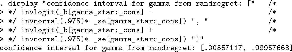
Because γ must lie between 0 and 1, the optimization uses an ancillary parameter with a logistic transformation during the optimization procedure: γ = exp(γ*)/{1 + exp (γ*)} = logit ^{− 1}(γ*) = invlogit(γ*), where γ* is an unbounded ancillary parameter. Normally, γ* is hidden from the output, but it can be shown using the option showancillary. The resulting γ* is displayed in the _cons variable of the gamma_star equation.

Finally, using $\widehat{{\gamma }^{*}}$ , we can obtain $\widehat{\gamma }$ back on the original scale from 0 to 1 by using the logistic transformation. It is displayed as gamma in the output. The standard error of gamma is computed using the delta method. To exemplify the last point, manually, it is possible to recover $\widehat{\gamma }$ (gamma) using (see [R] nlcom).

From the nlcom output, some immediate discrepancies are evident regarding the confidence interval (CI), where the upper bound violates the restriction that we imposed on γ. As Buis (2014) documented using the heckman command, the discrepancies in CI occur because nl computes the CI using $\widehat{\gamma }\hspace{0.17em}\pm \hspace{0.17em}{z}_p{\left\{\widehat{\text{Var}}(\widehat{\gamma })\right\}}^{1/2}$ . Accordingly, using the procedure of Buis (2007) and noting that the $\widehat{\gamma }$ and ${\left\{\widehat{\text{Var}}(\widehat{\gamma })\right\}}^{1/2}$ are stored in e(gamma) and e(gamma_sd), respectively, we can recover the CI of nlcom as follows.

On the other hand, randregret computes the CI using the endpoints of $\widehat{{\text{γ}}^{\ast }}$ and then transforms those endpoints back into the restricted space. Therefore, the CI is computed using invlogit $\left[{\gamma }^{*}\pm z_{\rho }{\left\{\mathrm{Var}\left({\widehat{\gamma }}^{*}\right)\right\}}^{1/2}\right]$ . We can replicate the CI produced by randregret manually as follows:

Even though both ways are asymptotically equivalent, in finite samples they are likely to differ. Moreover, the way used by randregret ensures that the restrictions imposed on the parameter are met by the CI too.

Additionally, randregret computes two LR tests for γ. As explained earlier, given that we are testing a null hypothesis at the boundaries of the parametric space, we need to adjust the critical value (Gutierrez, Carter, and Drukker 2001). This is why the test mentions a chibar2(01), which is a mixture of a ${\chi }_1^2$ (50%) and a ${\chi }_0^2$ (50%). From the test, we can see that the hypothesis for γ = 0 is rejected, meaning that there is statistical evidence in favor of the data being generated by regret minimization behavior and not from RUM. Besides, we can see that the hypothesis for γ = 1 cannot be rejected, meaning here that the GRRM model is not significantly different from the classical RRM. Finally, it is important to note that, as stated before, the conclusions derived from the LR test that randregret displays by default are only valid when no corrections to the variance–covariance matrix are implemented, which does not happen in this case. Hence, a Wald test is better suited in this context.

The µRRM model can be obtained by typing rrmfn(mu), implementing (7) as systematic regret. For this model, similar to the GRRM model, we use an ancillary parameter approach to bound the searching space of our algorithm for µ between 0 and M. The transformation used is µ = M × [exp(µ*)/{1 + exp(µ*)}] = M × {logit ^{− 1}(µ*)} = M × {invlogit(µ*)}, where ${\mu }^{\ast }$ is an unbounded ancillary parameter and M is equal to the upper bound of the searching space. The upper bound that we used in this case was equal to 10, as can be seen in the uppermu() option. From the output, we see that randregret first runs the classical RRM model and uses the common parameters with the µRRM model as starting points for the maximization procedure.

The resulting ${\widehat{\mu }}^{\ast }$ is displayed in the _cons variable of the mu_star equation because of the showancillary option. To recover the value of $\widehat{\mu }$ , randregret applies the transformation described above. The same procedure can be performed using nlcom in the same fashion as we did for the GRRM model, with the only difference being that we need to multiply by the defined upper bound of the searching space to recover the parameter $\widehat{\mu }$ correctly. The same discrepancies in the CI produced by nlcom are due to the matter explained earlier in the GRRM model context and can be addressed as stated.

Additionally, randregret shows the LR test results for testing µ = 1. We see that it is not possible to reject the hypothesis that µ is equal to 1 (p = 0.686), meaning that the model is statistically equivalent to the classical RRM. However, because we fit the model using a cluster–robust variance–covariance matrix, the inference derived from LR tests is no longer valid, and a Wald test should be performed instead. An important remark for practitioners is that if the maximum is reached at $\widehat{\mu }$ = M, it is highly likely that µ is tending to infinity. Therefore, as argued in van Cranenburgh, Guevara, and Chorus (2015), this fact suggests that there is evidence in favor that the choice behavior is better represented by a linear RUM model.

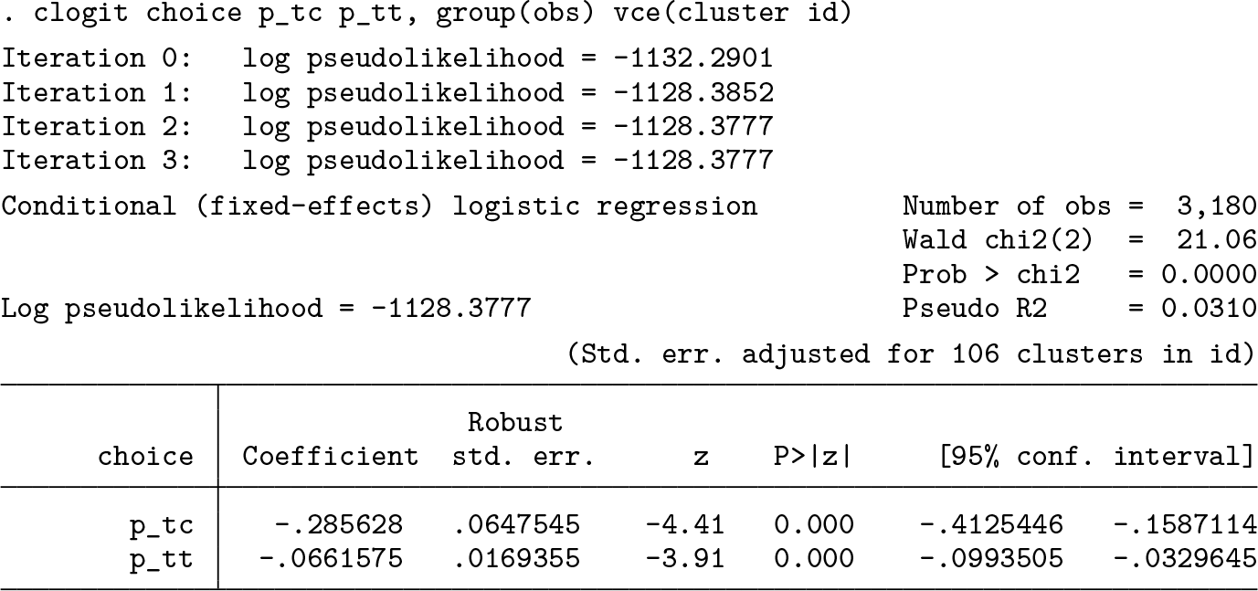
Finally, the PRRM model can be fit using the rrmfn(pure) option. As we mentioned before, this model is a particular case of the µRRM with µ arbitrarily small, and it is described by (9) and (10). Important differences with the common syntax need to be mentioned. Given that we need to feed the model with the expected signs of attributes, we do not include the explanatory variables conventionally. Instead, we split the attributes between the ones with an assumed positive sign and the ones with an assumed negative sign in the options positive() and negative(), respectively. In this particular case, both of our attributes are expected to have a negative sign because faster and cheaper routes are preferable to slower and costlier ones. Therefore, when the level on a nonchosen alternative increases, the regret decreases. Consequently, we need to include the two attributes as follows: negative(tc tt).

As mentioned in the footnote of the output, randregret performs the attribute transformation using (10). The transformed attributes are generated using the command randregret_pure. Afterwards, randregret simply invokes clogit to fit the model using these transformed attributes.

Additionally, for the sake of illustration, we will also fit the PRRM model using randregret_pure and clogit independently. The randregret_pure command can generate the transformed attributes described in (10). When dealing with a mix of positive and negative attributes, their transformations need to be created in two different runs of randregret_pure, that is to say, one for assumed positive attributes and the other for assumed negative attributes. In our case, all the attributes are assumed to have negative signs. Hence, we can create them in a single run of randregret_pure using the option signbeta(neg). Finally, given that the function will add the transformed attributes as new Stata variables, the user needs to provide a prefix to name and include them in the dataset. Consequently, we type prefix(p_) to declare that all the new attributes’ names will start with the p_ prefix.

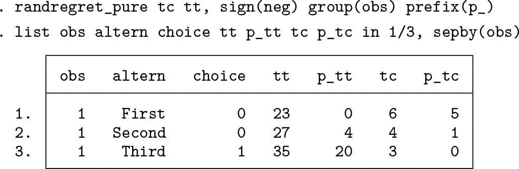
To further illustrate the process of generating the new attributes, we will follow the calculations in (10) to obtain the transformed attribute (p_tt) from the original attribute total time (tt) for the first choice situation (obs==1) of the first individual.

The new transformed attribute p_tt, conditional on an assumed negative sign from the original attribute, is given by $x_{i,tt,1}^{\text{PRRM}}={\displaystyle \sum }_{j\ne i}^3$ Subsequently, in matrix format, we will perform the following calculations to obtain p_tt.

$\begin{array}{l}{X}_{tt,1}^{\text{PRRM}}=\left(\begin{array}{l}{x}_{1,tt,1}^{\text{PRRM}}\hfill \\ x_{2,tt,1}^{\text{PRRM}}\hfill \\ x_{3,tt,1}^{\text{PRRM}}\hfill \end{array}\right)=\left(\begin{array}{c}\min \left(0,x_{2,tt,1}-x_{1,tt,1}\right)+\min \left(0,x_{3,tt,1}-x_{1,tt,1}\right)\\ \min \left(0,x_{1,tt,1}-x_{2,tt,1}\right)+\min \left(0,x_{3,tt,1}-x_{2,tt,1}\right)\\ \min \left(0,x_{1,tt,1}-x_{3,tt,1}\right)+\min \left(0,x_{2,tt,1}-x_{3,tt,1}\right)\end{array}\right)\\ =\left(\begin{array}{l}\min (0,27-23)+\min (0,35-23)\hfill \\ \min (0,23-27)+\min (0,35-27)\hfill \\ \min (0,23-35)+\min (0,27-35)\hfill \end{array}\right)\\ =\left(\begin{array}{c}0+0\\ -4+0\\ -12+-8\end{array}\right)=\left(\begin{array}{c}0\\ -4\\ -20\end{array}\right)\end{array}$

It is worth mentioning that randregret_pure flips the signs of the variables to be used directly in combination with clogit. This is because to obtain the choice probabilities using (11), we need to use the negative of (10), which is exactly what we achieve by invoking clogit using the transformed variables. Finally, we can check that we get the same results when running randregret using the rrmfn(pure) option and using randregret_pure together with clogit.

As we mentioned earlier, randregret also allows for the inclusion of ASC for all the models using (12). Below, we run a classic RRM model using the basealternative(1) option, which specifies that the first alternative is the reference for the ASC. We list the results here to illustrate the syntax only because the survey was implemented using nonlabeled alternatives.

To generate predictions, we can invoke randregretpred after running randregret. To illustrate this, we rerun the classical RRM model and generate two different predictions. First, using the option proba, we generate the prob variable, which contains the predicted probability of (4). Additionally, we also used the xb option to generate a variable containing the linear predicted systematic regret of (3).

11 Conclusions

We presented the randregret command, which allows the user to easily fit four different RRM models, namely, the classic RRM (Chorus 2010), the GRRM (Chorus 2014), the µRRM, and the PRRM (van Cranenburgh, Guevara, and Chorus 2015). We illustrated the results using stated choice discrete choice data in the context of route selection given in van Cranenburgh and Alwosheel (2019). Additionally, we have included additional LR tests that rely on the relationships among the models, which allows us to test whether the data are more likely to be generated by RRM or RUM choice behavior.

Supplemental Material

Supplemental Material, sj-zip-1-stj-10.1177_1536867X211045538 - randregret: A command for fitting random regret minimization models using Stata

Supplemental Material, sj-zip-1-stj-10.1177_1536867X211045538 for randregret: A command for fitting random regret minimization models using Stata by Álvaro A. Gutiérrez-Vargas, Michel Meulders and Martina Vandebroek in The Stata Journal