
Abstract
In this article, we describe a new command,
1 Introduction
In this article, we present a new command for estimating categorical proportions in the presence of misclassification error. The motivating case for the development and implementation of this command comes from substance use epidemiology. In this field of research, quantitative goals include measuring alcohol relative risks (RRs) and attributable fractions for specific diseases (for example, Rehm and Shield [2013]; Kehoe et al. [2012]; Meier et al. [2013]; Nelson et al. [2013]) and deriving public health guidelines for consumption (Kalinowski and Humphreys 2016). Furthermore, multinomial data and the potential for misclassification bias is commonplace in many disciplines, including medicine (for example, Chen et al. [2019]), education (for example, Goldstein, Browne, and Charlton [2018]), and marketing (for example, Gmehling and La Mura [2016]). The command we describe below implements the Bayesian model proposed by Swartz et al. (2004), which explicitly accounts for the possibility of misclassification error in a multinomial data setting. Ignoring the possibility of misclassification can lead to biased and inefficient estimates of proportions (Goldstein and Wolf 1977; Katz and McSweeney 1979; Schwartz 1985).
Bross (1954) laid out the framework for working with misclassification in the binary case. If validation data are available, both the misclassification rate and the binary proportion can be estimated (Tenenbein 1970). Without validation data, these parameters may be bounded or estimated from a fully Bayesian model (for example, Gaba and Winkler [1992]; Joseph, Gyorkos, and Coupal [1995]; Bollinger and van Hasselt [2017]). However, when data have more than two categories, misclassification is more challenging with complex and potentially asymmetric errors across categories, and a much larger parameter space needed to support underlying distributions. This latter consideration is a major reason why Bayesian approaches to the problem have been popular (see Pérez et al. [2007] for a review). One such approach is from Swartz et al. (2004), who focused on Bayesian identifiability with multinomial data. Swartz et al. (2004) extended work on the binary case approach using mixtures of Dirichlet distributions (Evans et al. 1996) and took advantage of increasing computational capability to apply Markov chains to estimate high-dimensional posterior distributions.
As noted above, our interest in the statistical problem of misclassification in multinomial data is associated with modeling alcohol exposure distributions. In this context, researchers often rely on a nationally representative self-reported survey data source. These data sources typically collect quantities (for example, number of drinks per drinking day) and frequencies (for example, number of drinking days) of alcohol consumption during some reference period (for example, past 30 days). Using these data, we can derive the average amount of alcohol consumed daily either in terms of grams per day or in terms of standard drinking units (that is, 1 standard drinking unit = 10 grams per day). Because many national drinking guidelines are framed in terms of the number of standard drinking units, it is natural to classify individuals according to a prespecified set of drinking unit ranges. For example, in the empirical applications below, we will categorize survey respondents as: i) nondrinkers; ii) persons who consume up to one drink per day; iii) persons who consume one to two drinks per day; iv) persons who consume two to three drinks per day; v) persons who consume three to four drinks per day; vi) persons who consume four to five drinks per day; and vii) persons who consume more than five drinks per day.
A common concern, however, is that there is underlying error in the amount of alcohol consumption reported by survey respondents and that this causes some individuals to be misclassified (Kilian et al. 2020). While triangulation methods have been proposed for addressing this concern (Rehm et al. 2010a; Parish et al. 2017), these methods have some important limitations. A typical triangulation approach uses data from a selfreported survey to measure the average amount of alcohol consumed and compares this with a less error-prone measure of average alcohol consumption, such as from national records of alcohol sales. The ratio of the total volume of alcohol sold nationally per capita divided by the average amount of alcohol reported in a representative survey provides a measurement of how much people are underreporting on average. For example, if this ratio is approximately two, then on average survey respondents are only reporting about half of what they actually drink. This ratio can then be used as a constant multiplier to upshift the distribution of alcohol consumption as measured by the survey (that is, double all respondents alcohol consumption). A key limitation associated with this approach is that it assumes that survey respondents underreport by a constant factor, which may be untrue. For example, it may be the case that more frequent drinkers underreport less than those drinkers who drink infrequently. Moreover, this approach implicitly assumes that there is no misclassification among nondrinkers. In the context of measuring alcohol-attributable fractions (AAFs), these limitations may be particularly important because prevalence estimates are used to weight the risk distribution and risks can vary substantially across the alcohol consumption distribution.
Swartz et al. (2004) provide a Bayesian misclassification method that can be used as an alternative method for adjusting the alcohol exposure distribution. As described below, the model is identified on the basis of constraints and by leveraging Bayesian priors. The Bayesian priors can be used to embed alternative assumptions about misclassification across the alcohol consumption distribution, and this provides greater flexibility over how the distribution is adjusted. Thus, this approach can be used to overcome the limitations of typical triangulation approaches.
2 The Swartz et al. (2004) model
2.1 The model
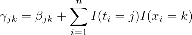
Let xi denote a multinomial variable that takes the values 1,…, m for the ith observation. The goal is to measure the probability that xi = j for j = 1,…, m. In the absence of misclassification, this would be a straightforward task (for example, the prevalence within each of the m categories would provide an unbiased estimator). However, in the presence of misclassification, xi is a fallible measure, and the proportion of the sample observed within each of the m categories may underor overstate the true prevalence. To develop a model that can correct for misclassification, Swartz et al. (2004) introduce a latent variable, denoted by ti , that indicates the correct classification for each observation and a set of misclassification probabilities, denoted by πkj ≡ Pr(xi = j | ti = k). Letting ρj ≡ Pr(ti = j), the likelihood function is
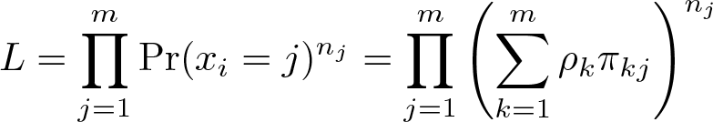
where nj
denotes the number of observations such that xi
= j. To complete the description of the model, the priors for

and

The Dirichlet distribution is a multivariate extension of the Beta distribution and is a commonly used prior distribution in many Bayesian applications. In
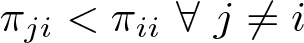
Swartz et al. (2004) provide a rigorous discussion of the concept of identification within the context of Bayesian modeling. In this discussion, they distinguish between two types of nonidentifiability. The first type corresponds with a more classical definition of parameter identification and can be resolved through the effective use of informative priors in the Bayesian specification of a prior and likelihood function. The second type is referred to as permutation-type nonidentifiability, and this type of nonidentifiability cannot be resolved through the use of priors. Mathematically, this type of nonidentifiability arises because any permutation of parameters that swaps the position of, for example, ρ
1 and ρ
2 while simultaneously swapping

To see how this constraint resolves the issue of identification, note that the likelihood function can be written in the presence of any constraint such that it returns zero for any parameter values that do not meet the constraint. For example, we could rewrite the likelihood as

If we now swap the positions of ρ
1 and ρ
2 while simultaneously swapping
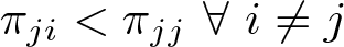
The intuition here is that constraining the misclassification parameters solves the identifiability issue by essentially eliminating from the parameter space arbitrary permutations. Additionally, specifying constraints on the misclassification parameters is also somewhat intuitive. In words, the first constraint considered in Swartz et al. (2004) says that it is most likely that the observed classification is correct and that it becomes sequentially less likely that the correct classification differs from the observed classification as classifications more distant from the observed data are considered. For example, if a person is actually in category 1, the probability of observing them in category 4 is less likely than observing them in category 3, which in turn is less likely than observing them in category 2. This type of constraint is likely reasonable in a variety of analysis contexts where the data are ordinal. The remaining constraints suggested by Swartz et al. (2004) are similar in spirit and are detailed below as part of our discussion of the command options.
While the number of categories is theoretically unbounded, ensuring these types of constraints on the parameter space are met becomes increasingly complex as larger numbers of categories are allowed. We have found that the model performs reasonably well with as many as eight categories. More may be possible, but convergence will become slow and impractical at higher numbers of categories.
Last, note that, while constraints resolve the permutation-type nonidentifiability, priors are still needed to ensure identification for this model. In fact, in our experience, stronger priors lead to significant improvements in the identification of the parameters of interest. Examples below illustrate this point.
2.2 Details of the Gibbs sampling algorithm
Swartz et al. (2004) outline a Gibbs sampling algorithm for simulating from the posterior distribution for
Step one
Sample from the discrete probability distribution for the latent unobserved variable, ti
, conditional on the observed variable, xi
, the corrected classification probabilities, ρ, and the misclassification probabilities,
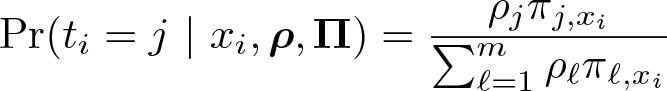
We sample from this discrete probability distribution in the usual way. Specifically, we first generate a pseudo–random uniform variate, u, and then for each j = 1,…, m, we check whether F (j − 1) ≤ u ≤ F (j), where F (a) ≡ Pr(ti ≤ a | xi,
Step two
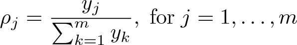
Sample from a Dirichlet distribution for the true but unobserved classification probabilities,
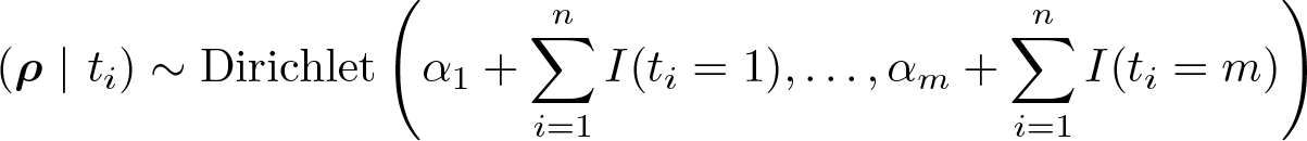
where I(c) denotes an indicator function that returns 1 if condition c is true and returns 0 otherwise. We follow a standard algorithm for generating pseudo–random Dirichlet variates, which starts by sampling from a Gamma distribution with shape set to
Step three
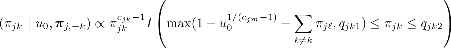
Sample from a truncated-Dirichlet distribution for the misclassification probabilities, πj , conditional on ti and xi ,

where
The truncation points for this distribution are how the constraints are captured in the Gibbs algorithm. In general, regardless of the specific constraint chosen, we can always capture the constraints by specifying a lower and upper bound, qjk 1 and qjk 2, for each of the misclassification probabilities such that 0 ≤ qjk 1 ≤ πjk ≤ qjk 2 ≤ 1.
As noted in Swartz et al. (2004), we can implement a rejection sampling scheme to sample from the truncated Dirichlet, which involves sampling from an untruncated Dirichlet and then checking whether the constraint is met. If not, then we continue sampling until the constraint is met. We use a more efficient sampling method instead, which is described in Damien and Walker (2001). This method essentially embeds a Gibbs algorithm within the larger Gibbs sampling scheme and is similar to an approach described in Swartz et al. (2004). In practice, however, we have found the Damien and Walker (2001) method to be more numerically stable.
This approach starts by sampling a pseudo–random uniform variate, u
0, between 0 and
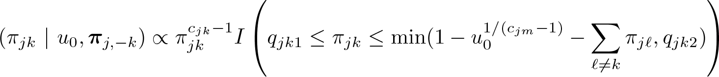
where
2.3 Model convergence and other calculations
The other major statistic that
Even when
3 The bamm command
3.1 Syntax
The syntax of
3.2 Required arguments
varname is the multinomial variable to be modeled. It must be integer valued and the minimum should be 1.
3.3 Options


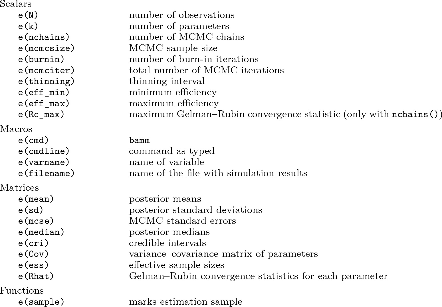
3.4 Stored results
3.5 Syntax for bammdx
The syntax of
Calling
3.6 Required arguments for bammdx
param_spec |
3.7 Options for bammdx
4 Examples
4.1 Simulation study
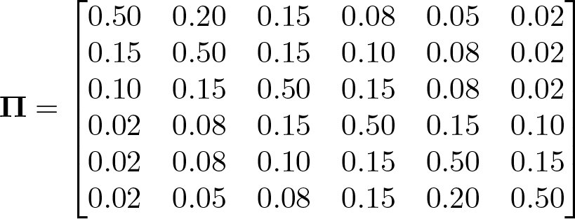
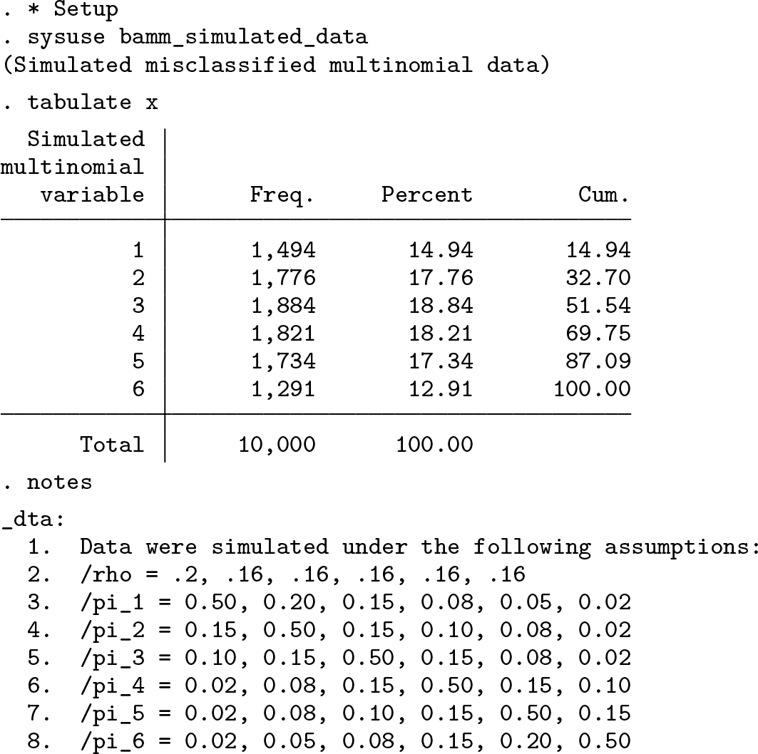
To illustrate the use of

and
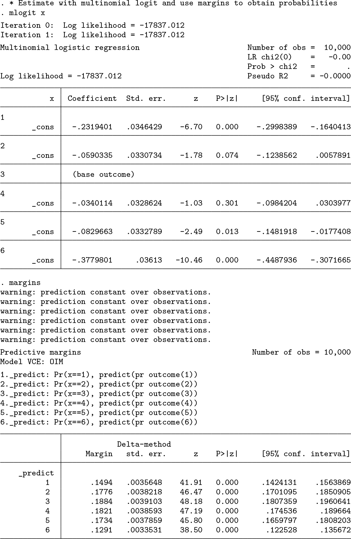
Tabulating this misclassified variate, we see that 15% of the sample is observed in the first category, between 17% and 19% of the sample are observed in the second through fifth categories, and 13% of the sample is observed in the sixth category. This shows us that the data are misclassified most strongly in the “tails” of the distribution or in the lowest and largest categories.
A naïve approach for estimating
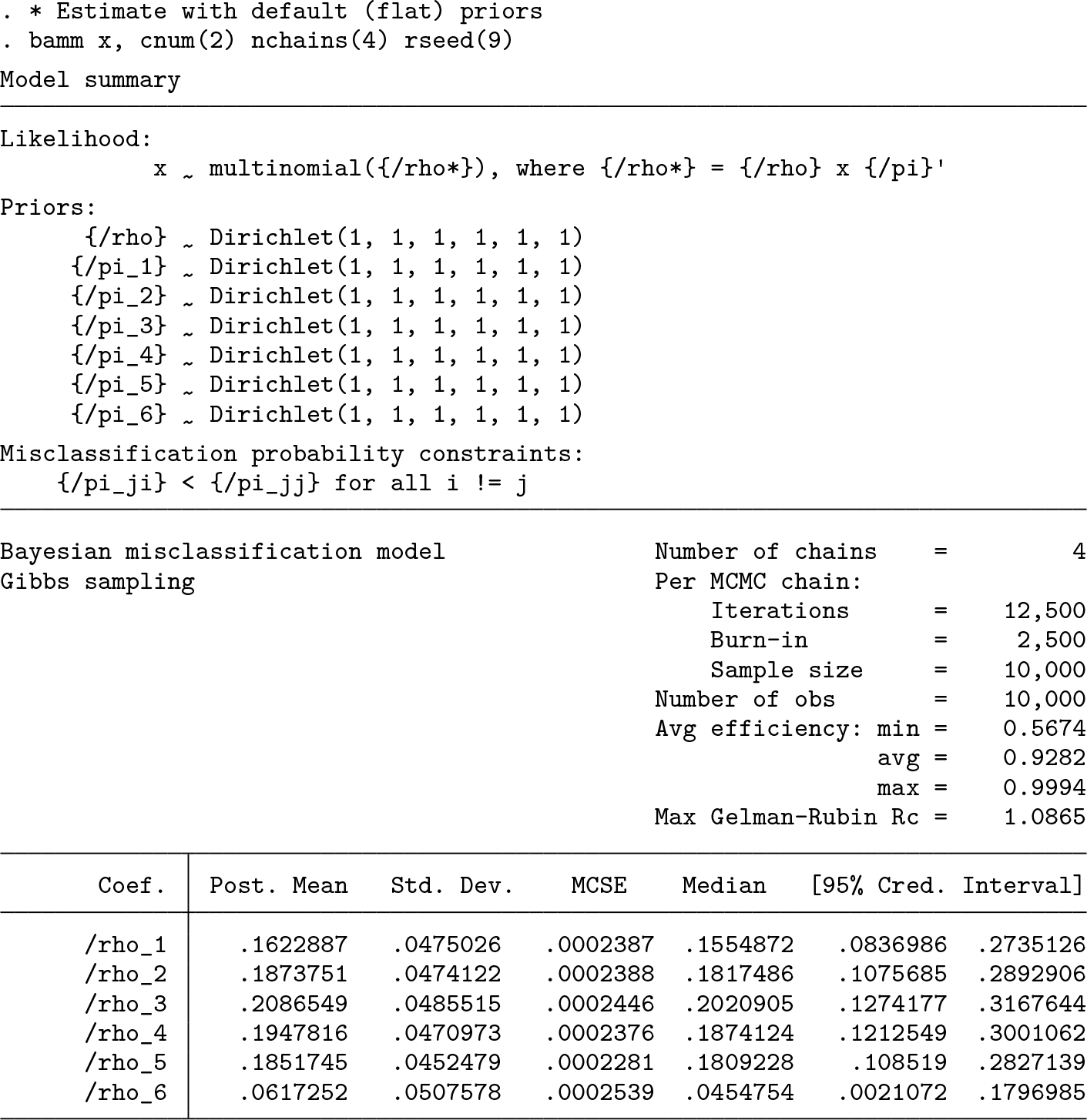
Although the model can be identified on the basis of the constraints alone, flat priors are not recommended (Swartz et al. 2004). To illustrate why, we show what happens when all the hyperparameters in the prior distribution are set equivalently to 1, which is the default. Using the second constraint, and sampling with four chains, we see that the model does slightly better than the naïve estimator, coming closer to the true parameter value for ρ
1 than the naïve estimator but performing much worse for ρ
6 than the naïve estimator. More importantly, while the posterior means are still inaccurate, the credible intervals are wider, representing greater uncertainty over the parameter values and do cover the true values of
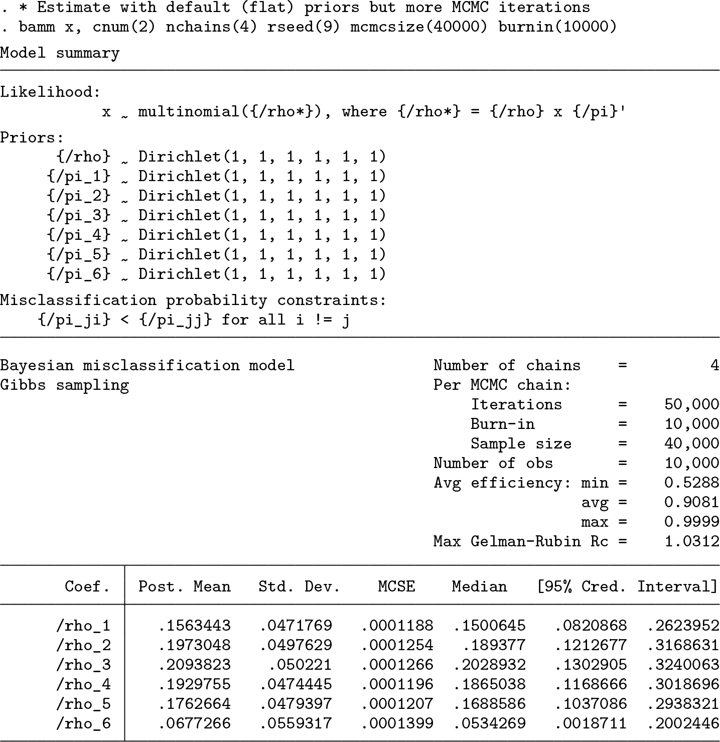
Below, we see that increasing the number of Monte Carlo repetitions leads to a smaller maximum
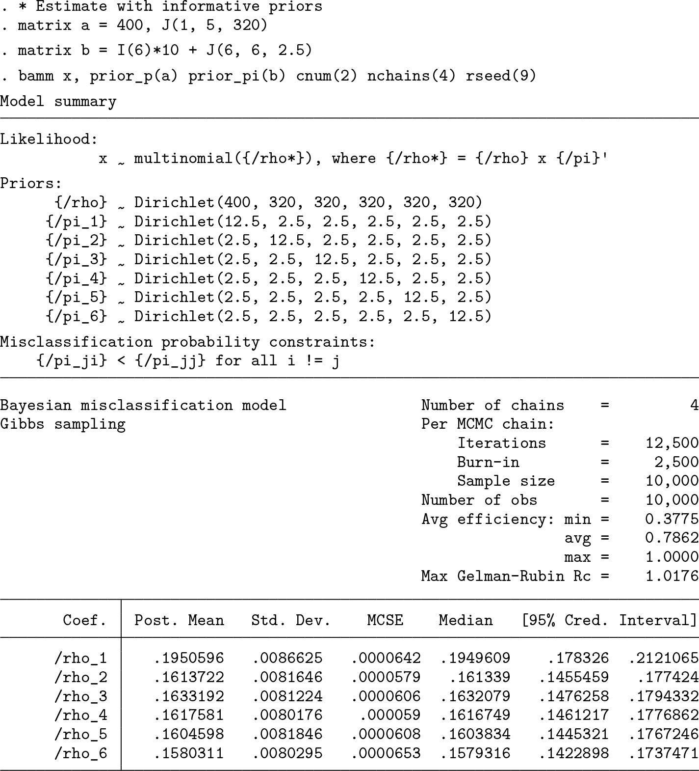
The last example shows what happens when we use informative priors for both the classification and misclassification probabilities. Specifically, we use a highly concentrated prior for the classification probabilities, which embeds an assumption that it is relatively more likely to be in the first classification than any other and that it is equally likely to be in the remaining classifications. Given our knowledge of the data-generating process, this is clearly a good assumption. We can see that the model now very accurately estimates
4.2 Empirical example
To provide an empirical example using
We accounted for binge drinking as described in Stahre et al. (2006). Straightforward quantity-frequency calculations multiply typical number of drinking days (F ) by the average number of drinks per day (Q). This may underestimate average daily consumption if respondents ever or frequently have days with higher than the average number of drinks per day reported. Because most surveillance surveys also provide data on the number of binge drinking days and average quantities consumed on binge drinking days, Stahre et al. (2006) recommend augmenting the basic quantity-frequency calculation as follows: define BQ as the binge quantity, BF as the binge frequency, and AF as the adjusted frequency of drinking (that is, AF = F − BF). Then the total drinks consumed can be calculated as Q × AF + BF × BQ.
As described in the introduction, triangulation methods require data on per capita sales (or other similar sources). We used alcohol sales data from the National Institute of Alcohol and Alcoholism (NIAAA) (Slater and Alpert 2021). These data show there were 2.38 gallons of ethanol sold in 2019 across all beverage types per person aged 14 years or older. We converted per capita gallons of ethanol sold to average grams of per capita ethanol per day. The multiplier used in the triangulation approach presented in this study was then derived as 75% of the average grams of ethanol sold per day in 2019 divided by the average grams of ethanol consumed per day in the BRFSS sample used. Adjusting to 75% of the average amount of alcohol sold provides a more conservative adjustment and is consistent with what other epidemiological studies have done (see for example, Esser et al. [2022]). While the per capita sales data do not account for nondrinkers, the denominator for the multiplier (that is, average daily alcohol consumption from the BRFSS) includes both drinkers and nondrinkers, with nondrinkers assigned zero grams of ethanol consumed per day. The BRFSS sample includes only individuals aged 18 to 64, and the per capita sales data represents sales per person aged 14 years or older. While the per capita sales data do provide separate estimates by beverage type, we did not consider different effects by beverage type for this analysis.
After deriving the triangulation multiplier, we multiplied the derived alcohol consumption variable by the multiplier. Other approaches (for example, Rehm et al. [2010a]; Parish et al. [2017]) adjust the parameters of estimated distributions (for example, the parameters of an estimated gamma distribution) rather than directly adjusting the data points themselves. We chose to directly adjust the data in this way for illustration purposes, because this allows us to provide the adjusted data to Stata users who can then apply our code examples and more easily replicate the examples in this article.
Using prevalence estimates (unadjusted, triangulation adjusted, and adjusted with
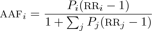
where Pi denotes the prevalence of drinking in the ith drinking category and RR i denotes the risk of liver cirrhosis mortality associated with drinking in category i. The formula used in this article decomposes the attributable fractions from each of the drinking categories as compared with no drinking. The total AAF can be calculated as the sum of the categorical-specific attributable fractions. Data on the RR of liver cirrhosis mortality were obtained from Rehm et al. (2010b).
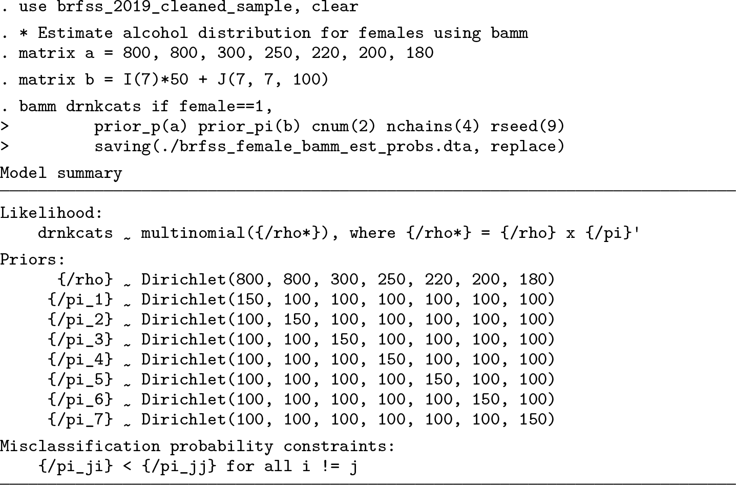
Below, we use

and
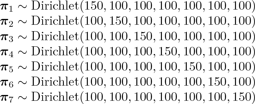
The prior for ρ reflects a prior belief that there is more underreporting among persons who are actually in higher drinking categories relative to those who are actually in lower drinking categories. The priors on πj for j = 1,…, 7 were chosen to be consistent with the second constraint, which we have used below.
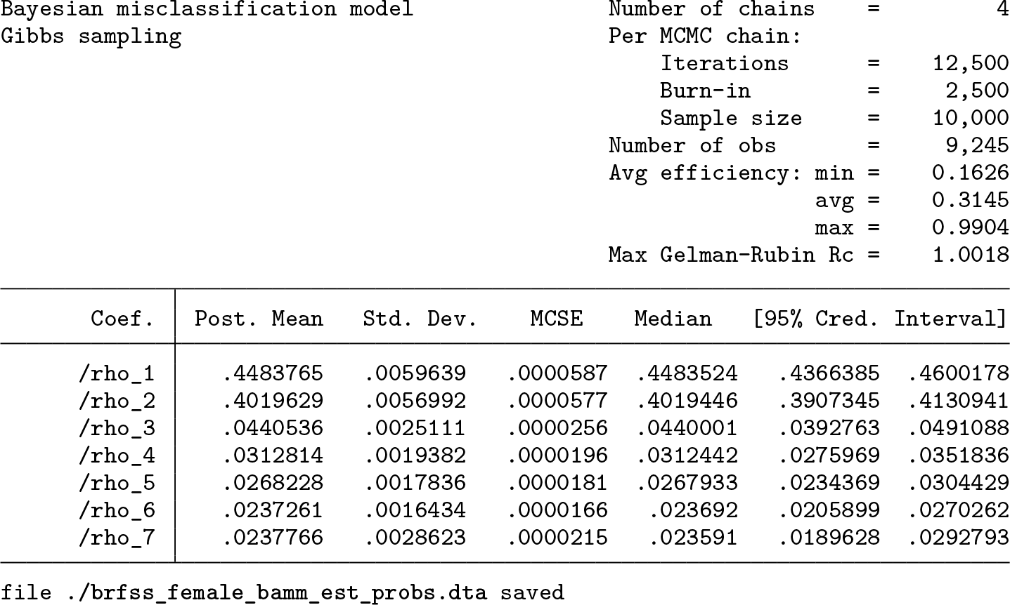
As can be seen in the output above, all parameters have
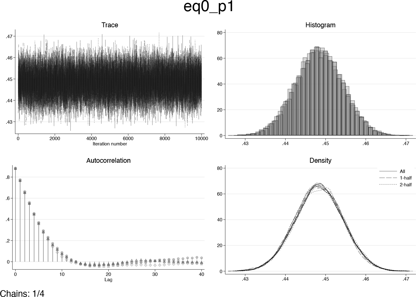
Diagnostic plots for ρ
1 after initial run of
Table 1 summarizes the results. Triangulation-based estimates do not adjust the prevalence of nondrinkers for either female or male respondents. This is because triangulation upshifts consumption by a constant factor, and zero multiplied by any number remains zero. Based on the priors chosen in this analysis,
Estimates of the AAF of liver cirrhosis mortality cases
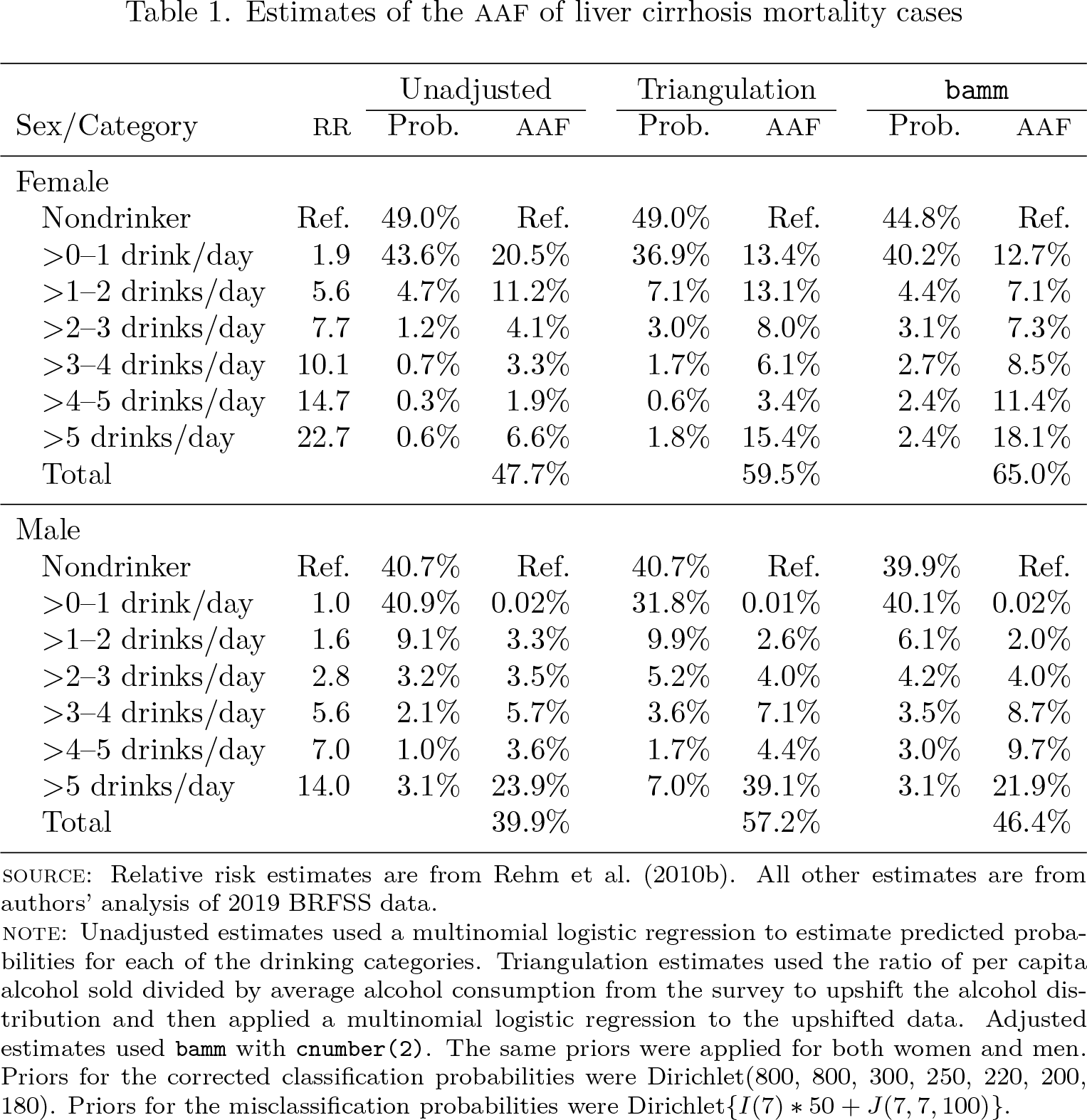
SOURCE: Relative risk estimates are from Rehm et al. (2010b). All other estimates are from authors’ analysis of 2019 BRFSS data.
NOTE: Unadjusted estimates used a multinomial logistic regression to estimate predicted probabilities for each of the drinking categories. Triangulation estimates used the ratio of per capita alcohol sold divided by average alcohol consumption from the survey to upshift the alcohol distribution and then applied a multinomial logistic regression to the upshifted data. Adjusted estimates used
5 Conclusion
This interplay between priors, credible interval width, and bias highlights the importance of the task of choosing and setting priors in empirical examples. Unfortunately, in most empirical applications, it is not likely that one can choose priors based on precise knowledge of the data-generating process, as is the case with the simulation study presented in this article. However, it may be possible to leverage external information to derive informative priors. For example, if a gold standard study exists demonstrating the degree to which a survey instrument misclassifies respondents, then results of this gold standard study could be used to derive informative priors.
The empirical study presented in this article provides some insight into the ways in which
While we have focused heavily on the use of
7 Programs and supplemental material
Supplemental Material, sj-zip-1-stj-10.1177_1536867X241233671 - A Bayesian method for addressing multinomial misclassification with applications for alcohol epidemiological modeling
Supplemental Material, sj-zip-1-stj-10.1177_1536867X241233671 for A Bayesian method for addressing multinomial misclassification with applications for alcohol epidemiological modeling by William J. Parish, Arnie Aldridge and Martijn van Hasselt in The Stata Journal
Footnotes
6 Acknowledgment
This work was supported by a research grant from the National Institute of Alcohol and Alcoholism (NIAAA: R01AA027796-01). The views expressed in this article are the authors’ own and do not necessarily represent the official views of the NIAAA.
7 Programs and supplemental material
To install the software files as they existed at the time of publication of this article, type
References
Supplementary Material
Please find the following supplemental material available below.
For Open Access articles published under a Creative Commons License, all supplemental material carries the same license as the article it is associated with.
For non-Open Access articles published, all supplemental material carries a non-exclusive license, and permission requests for re-use of supplemental material or any part of supplemental material shall be sent directly to the copyright owner as specified in the copyright notice associated with the article.