ddml: Double/debiased machine learning in Stata

Abstract

In this article, we introduce a package, ddml, for double/debiased machine learning in Stata. Estimators of causal parameters for five different econometric models are supported, allowing for flexible estimation of causal effects of endogenous variables in settings with unknown functional forms or many exogenous variables. ddml is compatible with many existing supervised machine learning programs in Stata. We recommend using double/debiased machine learning in combination with stacking estimation, which combines multiple machine learners into a final predictor. We provide Monte Carlo evidence to support our recommendation.

1 Introduction

Identification of causal effects frequently relies on an unconfoundedness assumption, which is that treatment or instrument assignment is sufficiently random given observed control covariates. Estimation of causal effects in these settings then involves conditioning on the controls. Unfortunately, estimators of causal effects that are insufficiently flexible to capture the effect of confounds generally do not produce consistent estimates of causal effects even when unconfoundedness holds. For example, Blandhol et al. (2022) highlight that two-stage least-squares estimands obtained after controlling linearly for confounds do not generally correspond to weakly causal effects even when instruments are valid conditional on controls. Even in the ideal scenario, where theory provides few relevant controls, theory rarely specifies the exact nature of confounding. Thus, applied empirical researchers wishing to exploit unconfoundedness assumptions to learn causal effects face a nonparametric estimation problem.

Traditional nonparametric estimators suffer greatly under the curse of dimensionality and are quickly impractical in the frequently encountered setting with multiple observed covariates. ¹ These difficulties leave traditional nonparametric estimators essentially inapplicable in the presence of increasingly large and complex datasets, for example, textual confounders as in Roberts, Stewart, and Nielsen (2020) or digital trace data (Hangartner, Kopp, and Siegenthaler 2021). Tools from supervised machine learning have been put forward as alternative estimators. These approaches are often more robust to the curse of dimensionality via the exploitation of regularization assumptions. A prominent example of a machine learning-based causal-effects estimator is the post double selection lasso (PDS-lasso) of Belloni, Chernozhukov, and Hansen (2014), which fits auxiliary lasso regressions of the outcome and treatments against a menu of transformed controls. Under an approximate sparsity assumption, which posits that the data-generating process (DGP) can be approximated well by relatively few terms included in the menu, this approach allows for precise treatment-effects estimation. The lasso can also be used for approximating optimal instruments (Belloni et al. 2012). Lasso-based approaches for estimation of causal effects have become a popular strategy in applied econometrics (for example, Gilchrist and Sands [2016]; Dhar, Jain, and Jayachandran [2022]), partially facilitated by the availability of software programs in Stata (pdslasso, Ahrens, Hansen, and Schaffer 2018) and R (hdm, Chernozhukov, Hansen, and Spindler 2016).

Although approximate sparsity is a weaker regularization assumption than assuming a linear functional form that depends on a known low-dimensional set of variables, it may not be suitable in a wide range of applications. For example, Giannone, Lenza, and Primiceri (2021) argue that approximate sparsity may provide a poor description in several economic examples. Thus, there is a potential benefit to expanding the set of regularization assumptions and correspondingly considering a larger set of machine learners, including, for example, random forests, gradient boosting, and neural networks. While the theoretical properties of these estimators are an active research topic (see, for example, Athey, Tibshirani, and Wager [2019] and Farrell, Liang, and Misra [2021]), machine learning methods are widely adopted in industry and practice for their empirical performance. To facilitate their application for causal inference in common econometric models, Chernozhukov et al. (2018) propose double/debiased machine learning (DDML), which exploits Neyman orthogonality of estimating equations and cross-fitting to formally establish asymptotic normality of estimators of causal parameters under relatively mild convergence rate conditions on nonparametric estimators.

DDML increases the set of machine learners that researchers can leverage for estimation of causal effects. Deciding which learner is most suitable for a particular application is difficult, however, because researchers are rarely certain about the structure of the underlying DGP. A practical solution is to construct combinations of a diverse set of machine learners using stacking (Wolpert 1992; Breiman 1996). Stacking is a meta-learner given by a weighted sum of individual machine learners (the “base learners”). When the weights corresponding to the base learners are chosen to maximize out-of-sample predictive accuracy, this approach hedges against the risk of relying on any particular poorly suited or ill-tuned machine learner.

In this article, we introduce the package ddml, which implements DDML for Stata. ² ddml adds to a few programs for causal machine learning in Stata (Ahrens, Hansen, and Schaffer 2018). We briefly summarize the four main features of the program:

ddml supports flexible estimators of causal parameters in five econometric models: a) the partially linear model, b) the interactive model (for binary treatment), c) the partially linear instrumental-variables (IV) model, d) the flexible partially linear IV model, and e) the interactive IV model (for binary treatment and instrument).

ddml supports data-driven combinations of multiple machine learners via stacking by leveraging pystacked (Ahrens, Hansen, and Schaffer 2023), our complementary Stata front-end relying on the Python library scikit-learn (Pedregosa et al. 2011; Buitinck et al. 2013). ddml also supports two novel approaches to pairing DDML with stacking introduced in Ahrens et al. (2024): Short-stacking takes a shortcut by leveraging the cross-fitted predicted values for estimating the stacking weights, and pooled stacking enforces common weights across cross-fitting folds.

Aside from pystacked, ddml can be used in combination with many other existing supervised machine learning programs available in or via Stata. ddml has been tested with lassopack (Ahrens, Hansen, and Schaffer 2020), rforest (Schonlau and Zou 2020), svmachines (Guenther and Schonlau 2018), and parsnip (Huntington-Klein 2021). Indeed, the requirements for compatibility with ddml are minimal: any eclass program with the Stata-typical “regress y x” syntax, support for if conditions, and a postestimation predict command is compatible with ddml.

ddml provides flexible multiline syntax and short one-line syntax. The multiline syntax offers a wide range of options, guides the user through the DDML algorithm step by step, and includes auxiliary programs for storing, loading, and displaying additional information. We also provide a complementary one-line version called qddml (“quick” ddml), which uses a similar syntax to pdslasso and ivlasso (Ahrens, Hansen, and Schaffer 2018).

The article proceeds as follows. Section 2 outlines DDML for the partially linear and interactive models under conditional unconfoundedness assumptions. Section 3 outlines DDML for IV models. Section 4 discusses how stacking can be combined with DDML and provides evidence from Monte Carlo simulations illustrating the advantages of DDML with stacking. Section 5 explains the features, syntax, and options of the command. Section 6 demonstrates the command’s usage with two applications.

2 DDML with conditional unconfoundedness

This section discusses DDML for the partially linear model and the interactive model in turn. The exposition follows Chernozhukov et al. (2018). Both models are special cases of the general causal model

$Y=f_0(D,\mathit{X}, U)$

1

where f ₀ is a structural function, Y is the outcome, D is the variable of interest, X are observed covariates, and U are all unobserved determinants of Y (that is, other than D and X ). ³ The key difference between the partially linear model and the interactive model is their positions in the tradeoff between functional form restrictions on f ₀ and restrictions on the joint distribution of observables (D, X ) and unobservables U. For both models, we highlight key parameters of interest, state sufficient identifying assumptions, and outline the corresponding DDML estimator. A random sample ${\left\{\left(Y_i,\hspace{0.17em}{D}_i,\hspace{0.17em}{\mathit{X}}_i\right)\right\}}_{i=1}^n$ from (Y, D, X ) is considered throughout.

2.1 The partially linear model (partial)

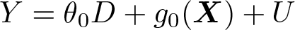
The partially linear model imposes the estimation model

$Y={\theta }_{0}D+g_0(\mathit{X}) +U$

2

where θ ₀ is a fixed unknown parameter. The key feature of the model is that the controls X enter through the unknown and potentially nonlinear function g ₀. Note that D is not restricted to be binary and may be discrete, continuous, or mixed. For simplicity, we assume that D is a scalar, although ddml allows for multiple treatment variables in the partially linear model.

The parameter of interest is θ ₀, the causal effect of D on Y . ⁴ The key identifying assumption is given in assumption 1. ⁵

Assumption 1 (Conditional orthogonality). E{Cov(U, D| X )} = 0.

To show identification of θ ₀, consider the score

$\psi (\mathit{W};\theta , m, \mathcal{l}) = [Y-\mathcal{l}(\mathit{X})-\theta \{D-m(\mathit{X})\}]\{D-m(\mathit{X})\}$

3

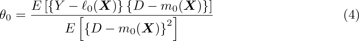
where W ≡ (Y, D, X ) and ℓ and m are nuisance functions. Letting m ₀( X ) ≡ E(D| X ) and ℓ ₀( X ) ≡ E(Y| X ), note that

$E\{\psi (\mathit{W};{\theta }_0, m_0, {\mathcal{l}}_0)\}= 0$

by assumption 1. When, in addition, E[Var(D| X )] ≠ 0, we get

${\theta }_0 = \frac{E\left[\left\{Y - {\mathcal{l}}_0(\mathit{X})\right\}\left\{D - m_0(\mathit{X})\right\}\right]}{E\left[{\left\{D - m_0(\mathit{X})\right\}}^2\right]}$

4

Equation (4) is constructive in that it motivates estimation of θ ₀ via a simple twostep procedure: First, estimate the conditional expectation of Y given X (that is, ℓ ₀) and of D given X (that is, m ₀) using appropriate nonparametric estimators (for example, machine learners). Second, residualize Y and D by subtracting their respective conditional expectation function (CEF) estimates, and regress the resulting CEF residuals of Y on the CEF residuals of D. This approach is fruitful when the estimation error of the first step does not propagate excessively to the second step. DDML leverages two key ingredients to control the impact of the first-step estimation error on the second-step estimate: 1) second-step estimation based on Neyman orthogonal scores and 2) crossfitting. As shown in Chernozhukov et al. (2018), this combination facilitates the use of any nonparametric estimator that converges sufficiently quickly in the first step and potentially opens the door for the use of many machine learners.

Neyman orthogonality refers to a property of score functions ψ that ensures local robustness to estimation errors in the first step. Formally, it requires that the Gateaux derivative with respect to the nuisance functions evaluated at the true values is meanzero. In the context of the partially linear model, this condition is satisfied for the moment condition (3),

${\partial }_r(E[\psi \{W;{\theta }_0, m_0+r(m-m_0), {\mathcal{l}}_0+r(\mathcal{l}-{\mathcal{l}}_0)\}]){|}_{r=0}=0$

where the derivative is with respect to the scalar r and evaluated at r = 0. Heuristically, we can see that this condition alleviates the impact of noisy estimation of nuisance functions as local deviations of the nuisance functions away from their true values leave the moment condition unchanged. We refer to Chernozhukov et al. (2018) for a detailed discussion but highlight that all score functions discussed in this article are Neyman orthogonal.

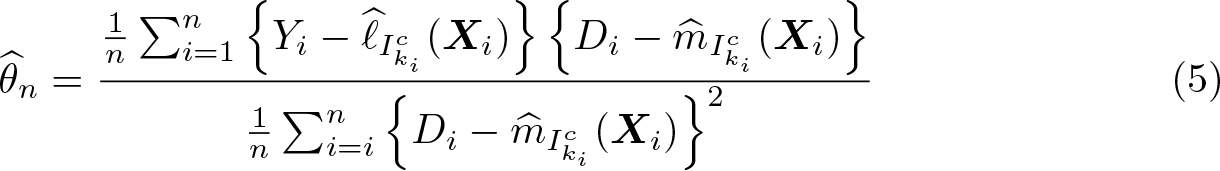
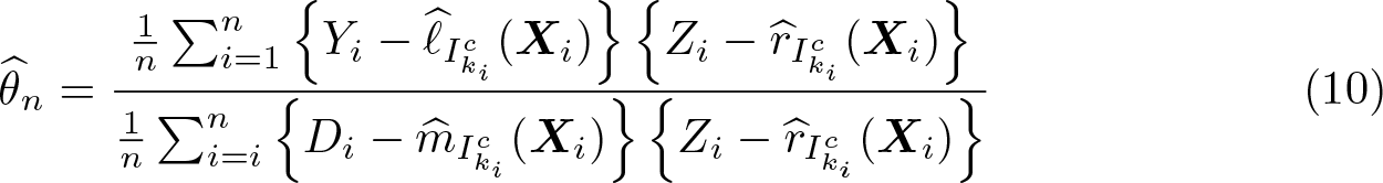
Cross-fitting ensures independence between the estimation error from the first step and the regression residual in the second step. To implement cross-fitting, we randomly split the sample into K evenly sized folds, denoted as I ₁ ,…, I_K . For each fold k, the conditional expectations ℓ ₀ and m ₀ are estimated using only observations not in the kth fold—that is, in $I_k^c\hspace{0.17em}\equiv I\backslash I_k$ —resulting in ${\widehat{\mathcal{l}}}_{I_k^c}$ and ${\widehat{m}}_{I_k^c}$ , respectively, where the subscript $I_k^c$ indicates the subsample used for estimation. The out-of-sample predictions for an observation i in the kth fold are then computed via ${\widehat{\mathcal{l}}}_{I_k^c}({\mathit{X}}_i)$ and ${\widehat{m}}_{I_k^c}({\mathit{X}}_i)$ . Repeating this procedure for all K folds then allows for computation of the DDML estimator for θ ₀:

${\widehat{\theta }}_n = \frac{\frac{1}{n}{\displaystyle {\sum }_{i=1}^n\left\{Y_i - {\widehat{\mathcal{l}}}_{I_{k_i}^c}\left({\mathit{X}}_i\right)\right\}}\left\{D_i - {\widehat{m}}_{I_{k_i}^c}\left({\mathit{X}}_i\right)\right\}}{\frac{1}{n}{\displaystyle {\sum }_{i=1}^n{\left\{D_i - {\widehat{m}}_{I_{k_i}^c}\left({\mathit{X}}_i\right)\right\}}^2}}$

5

where k_i denotes the fold of the ith observation. ⁶

We summarize the DDML algorithm for the partially linear model in algorithm 1: ⁷

Algorithm 1: DDML for the partially linear model

Split the sample ${\left\{\left(Y_i,\hspace{0.17em}{D}_i,\hspace{0.17em}{\mathit{X}}_i\right)\right\}}_{i=1}^n$ randomly in K folds of approximately equal size. Denote I_k the set of observations included in fold k and $I_k^c$ its complement.

1. For each k ∊ {1,…, K}:

Fit a CEF estimator to the subsample $I_k^c$ using Y_i as the outcome and X _i as predictors. Obtain the out-of-sample predicted values ${\widehat{\mathcal{l}}}_{I_k^c}({\mathit{X}}_i)$ for i ∊ I_k .

Fit a CEF estimator to the subsample $I_k^c$ using D_i as the outcome and X _i as predictors. Obtain the out-of-sample predicted values ${\widehat{m}}_{I_k^c}({\mathit{X}}_i)$ for i ∊ I_k .

2. Compute (5).

Chernozhukov et al. (2018) give conditions on the joint distribution of the data, particularly on g ₀ and m ₀, and properties of the nonparametric estimators used for CEF estimation, such that ${\widehat{\theta }}_n$ is consistent and asymptotically normal. Standard errors are equivalent to the conventional linear regression standard errors of $Y_i-\hspace{0.17em}{\widehat{\mathcal{l}}}_{I_{k_i}^c}({\mathit{X}}_i)$ on $D_i-\hspace{0.17em}{\widehat{m}}_{I_{k_i}^c}({\mathit{X}}_i)$ . ddml computes the DDML estimator for the partially linear model using Stata’s regress command. All standard errors available for linear regression in Stata are also available in ddml, including different heteroskedasticity and cluster–robust standard errors. ⁸

Remark 1: Number of folds

The number of cross-fitting folds is a necessary tuning choice. Theoretically, any finite value is admissible. Chernozhukov et al. (2018) report in remark 3.1 that four or five folds perform better than only using K = 2. Based on our simulation experience, we find that more folds tend to lead to better performance because more data are used for estimation of CEFs, especially when the sample size is small. We believe that more work on setting the number of folds would be useful but believe that setting K = 5 is likely a good baseline in many settings.

Remark 2: Cross-fitting repetitions

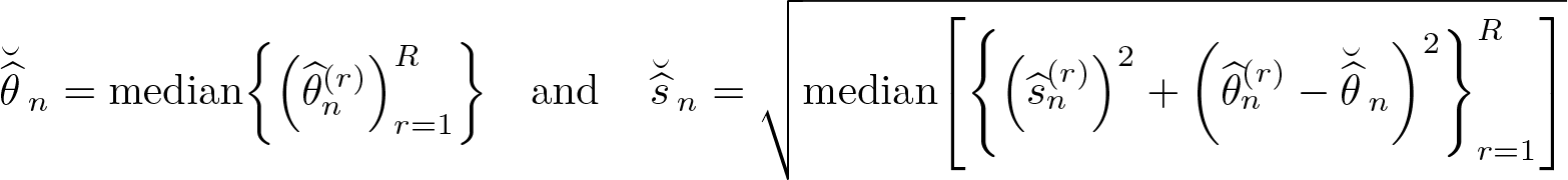
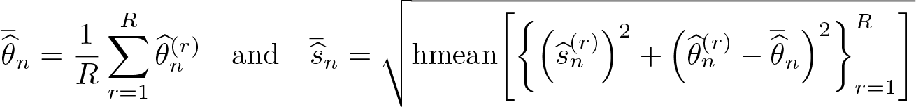
DDML relies on randomly splitting the sample into K folds. We recommend running the cross-fitting procedure more than once using different random folds to assess randomness introduced via the sample splitting. ddml facilitates this using the rep() option, which automatically fits the same model multiple times and combines the resulting estimates to obtain the final estimate. By default, ddml reports the median over cross-fitting repetitions. ddml also supports the average of estimates. Specifically, let ${\widehat{\theta }}_n^{(r)}$ denote the DDML estimate from the rth cross-fit repetition, and let ${\widehat{s}}_n^{(r)}$ denote its associated standard-error estimate with r = 1,…, R. The aggregate median point estimate and associated standard error are defined as

${\stackrel{⌣}{\widehat{\theta }}}_n = \mathrm{median}\left\{{\left({\widehat{\theta }}_n^{(r)}\right)}_{r=1}^R\right\} \hspace{0.17em}\text{and}\hspace{0.17em}{\stackrel{⌣}{\widehat{s}}}_n = \sqrt{\mathrm{median}\left[{\left\{{\left({\widehat{s}}_n^{(r)}\right)}^2+{\left({\widehat{\theta }}_n^{(r)}-{\stackrel{⌣}{\widehat{\theta }}}_n\right)}^2\right\}}_{r=1}^R\right]}$

The aggregate mean point estimate and associated standard error are calculated as

${\overline{\widehat{\theta }}}_n = \frac{1}{R}{\displaystyle \sum _{r=1}^R{\widehat{\theta }}_n^{(r)}}\text{ and }\hspace{1em}{\overline{\widehat{s}}}_n = \sqrt{\text{ hmean }\left[{\left\{{\left({\widehat{s}}_n^{(r)}\right)}^2 + {\left({\widehat{\theta }}_n^{(r)} - {\overline{\widehat{\theta }}}_n\right)}^2\right\}}_{r=1}^R\right]}$

where hmean is the harmonic mean. ⁹

Remark 3: Cluster-dependence and folds

Under cluster-dependence, we recommend randomly assigning folds by cluster; see fcluster().

2.2 The interactive model (interactive)

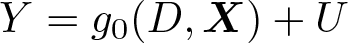
The interactive model is given by

$Y=g_0(D,\mathit{X}) +U$

6

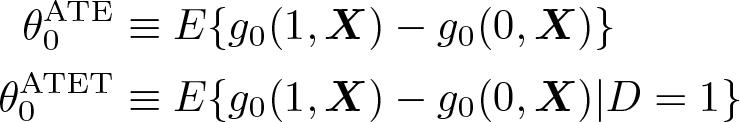
where D takes values in {0, 1}. The key deviations from the partially linear model are that D must be a scalar binary variable and that D is not required to be additively separable from the controls X . In this setting, the parameters of interest we consider are

$\begin{array}{l}\hspace{0.17em}{\theta }_0^{\text{ATE}}\equiv E\left\{g_0(1,\mathit{X})\hspace{0.17em}-\hspace{0.17em}{g}_0(0,\mathit{X})\right\}\\ {\theta }_0^{\text{ATET}}\equiv E\left\{g_0(1,\mathit{X})\hspace{0.17em}-\hspace{0.17em}{g}_0(0,\mathit{X})\mid D=1\right\}\end{array}$

which correspond to the average treatment effect (ATE) and average treatment effect on the treated (ATET), respectively.

Assumptions 2 and 3 below are sufficient for identification of the ATE and ATET. Note that the conditional mean independence condition stated here is stronger than the conditional orthogonality assumption sufficient for identification of θ ₀ in the partially linear model.

Assumption 2 (Conditional mean independence). E(U|D, X ) = 0.

Assumption 3 (Overlap). Pr(D = 1| X ) ∊ (0, 1) with probability 1.

Under assumptions 2 and 3, we have

$E(Y|D,\mathit{X}) =E\{g_0(D,\mathit{X})|D,\mathit{X}\}+E(U|D,\mathit{X}) =g_0(D,\mathit{X})$

so that identification of the ATE and ATET immediately follows from their definitions. ¹⁰

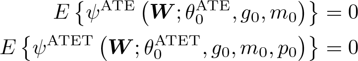
In contrast to section 2.1, second-step estimators are not directly based on the moment conditions used for identification. Additional care is needed to ensure local robustness to first-stage estimation errors (that is, Neyman orthogonality). In particular, the Neyman orthogonal score for the ATE that Chernozhukov et al. (2018) consider is the efficient influence function of Hahn (1998),

${\psi }^{\text{ATE}}(\mathit{W};\theta ,g,m) = \frac{D\{Y-g(1,\mathit{X})\}}{m(\mathit{X})} - \frac{(1-D)\{Y-g(0,\mathit{X})\}}{1-m(\mathit{X})} \hspace{0.17em}+\hspace{0.17em} g(1,\mathit{X}) - g(0,\mathit{X})- \theta$

where W ≡ (Y, D, X ). Similarly for the ATET,

${\psi }^{\mathrm{ATET}}(\mathit{W};\theta ,g,m,p)\hspace{0.17em}=\hspace{0.17em}\frac{D\{Y-g(0,\mathit{X})\}}{p}\hspace{0.17em}-\hspace{0.17em}\frac{m(\mathit{X})(1-D)\{Y-g(0,\mathit{X})\}}{p\{1-m(\mathit{X})\}}\hspace{0.17em}- \frac{D\theta }{p}$

Importantly, for g ₀(D, X ) ≡ E(Y |D, X ), m ₀( X ) ≡ E(D| X ), and p ₀ ≡ E(D), assumptions 2 and 3 imply

$\begin{array}{l}\hspace{0.17em}E\left\{{\psi }^{\text{ATE}}\left(\mathit{W};{\theta }_0^{\text{ATE}},\hspace{0.17em}{g}_0,m_0\right)\right\} = 0\\ E\left\{{\psi }^{\text{ATET}}\left(\mathit{W};{\theta }_0^{\text{ATET}},\hspace{0.17em}{g}_0,m_0,p_0\right)\right\} = 0\end{array}$

and we also have that the Gateaux derivative of each condition with respect to the nuisance parameters (g ₀ , m ₀ , p ₀) is zero.

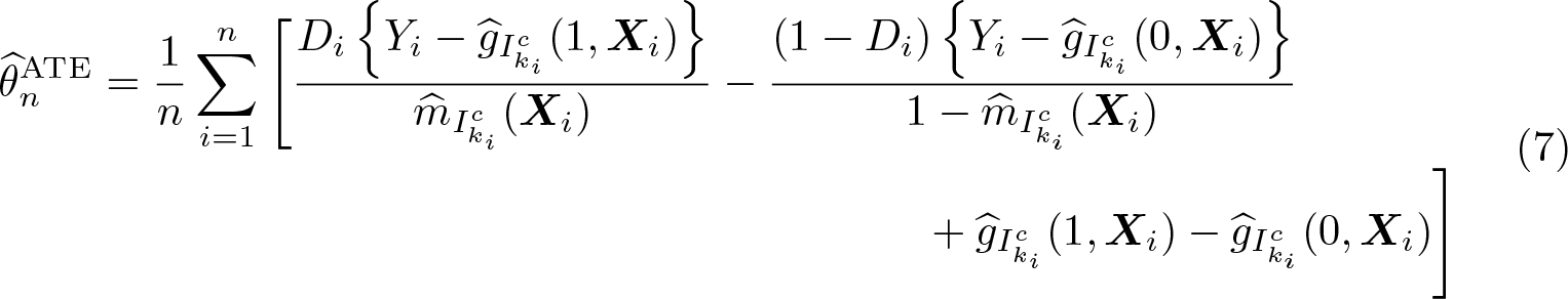
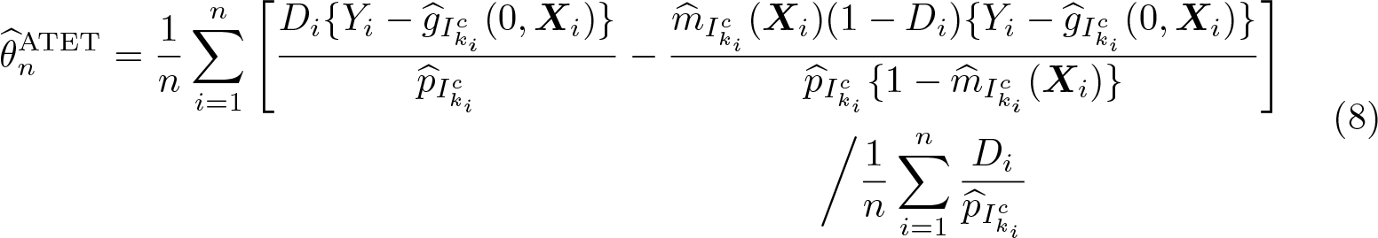
As before, the DDML estimators for the ATE and ATET leverage cross-fitting. The DDML estimators of the ATE and ATET based on ψ ^ATE and ψ ^ATET are

${\widehat{\theta }}_n^{\text{ATE}} = \frac{1}{n}{\displaystyle \sum _{i=1}^n[\frac{D_i\left\{Y_i - {\widehat{g}}_{I_{k_i}^c}\left(1,{\mathit{X}}_i\right)\right\}}{{\widehat{m}}_{I_{k_i}^c}\left({\mathit{X}}_i\right)} - \frac{\left(1 - D_i\right)\left\{Y_i - {\widehat{g}}_{I_{k_i}^c}\left(0,{\mathit{X}}_i\right)\right\}}{1 - {\widehat{m}}_{I_{k_i}^c}\left({\mathit{X}}_i\right)}} + {\widehat{g}}_{I_{k_i}^c}\left(1,{\mathit{X}}_i\right) - {\widehat{g}}_{I_{k_i}^c}\left(0,{\mathit{X}}_i\right)]$

7

${\widehat{\theta }}_n^{\text{ATET}} = \frac{1}{n}{\displaystyle \sum _{i=1}^n\left[\frac{D_i\left\{Y_i - {\widehat{g}}_{I_{k_i^c}^c}\left(0,{\mathit{X}}_i\right)\right\}}{{\widehat{p}}_{I_{k_i}^c}} - \frac{{\widehat{m}}_{I_{k_i}^c}\left({\mathit{X}}_i\right)\left(1 - D_i\right)\left\{Y_i - {\widehat{g}}_{I_{k_i}^c}\left(0,{\mathit{X}}_i\right)\right\}}{{\widehat{p}}_{I_{k_i}^c}\left\{1 - {\widehat{m}}_{I_{k_i}^c}\left({\mathit{X}}_i\right)\right\}}\right]}\hspace{0.17em}/\hspace{0.17em}\frac{1}{n}{\displaystyle \sum _{i=1}^n\frac{D_i}{{\widehat{p}}_{I_{k_i}^c}}}$

8

where ${\widehat{g}}_{I_k^c}$ and ${\widehat{m}}_{I_k^c}$ are cross-fitted estimators for g ₀ and m ₀ as defined in section 2.1. Because D is binary, the cross-fitted values ${\widehat{g}}_{I_k^c}(1,\mathit{X})$ and ${\widehat{g}}_{I_k^c}(0,\mathit{X})$ are computed by using only treated and untreated observations, respectively. ${\widehat{p}}_{I_k^c}$ is a cross-fitted estimator of the unconditional treatment probability.

ddml supports heteroskedasticity and cluster–robust standard errors for ${\widehat{\theta }}_n^{\text{ATET }}$ and ${\widehat{\theta }}_n^{\text{ATET }}$ . The algorithms for estimating the ATE and ATET are conceptually similar to algorithm 1. We delegate the detailed outline to algorithm A.1 in the online appendix. Mean and median aggregation over cross-fitting repetitions are implemented as outlined in remark 2.

3 DDML with IV

This section outlines the partially linear IV model, the flexible partially linear IV model, and the interactive IV model. The discussion is again based on Chernozhukov et al. (2018). As in the previous section, each model is a special case of the general causal model (1). The discussion in this section differs from the preceding section in that identifying assumptions leverage IVs Z . The two partially linear IV models assume strong additive separability as in (2), while the interactive IV model allows for arbitrary interactions between the treatment D and the controls X as in (6). The flexible partially linear IV model allows for approximation of optimal instruments ¹¹ as in Belloni et al. (2012) and Chernozhukov, Hansen, and Spindler (2015a) but relies on a stronger independence assumption than the partially linear IV model. Throughout this discussion, we consider a random sample ${\left\{\left(Y_i,D_i,{\mathit{X}}_i,Z_i\right)\right\}}_{i=1}^n$ from (Y, D, X , Z ).

3.1 Partially linear IV model (iv)

The partially linear IV model considers the same functional form restriction on the causal model as the partially linear model in section 2.1. Specifically, the partially linear IV model maintains

$Y={\theta }_{0}D+g_0(\mathit{X}) +U$

where θ ₀ is the unknown parameter of interest. ¹²

The key deviation from the partially linear model is that the identifying assumptions leverage IVs Z instead of directly restricting the dependence of D and U. For ease of exposition, we focus on scalar-valued instruments in this section, but we emphasize that ddml for partially linear IV supports multiple IVs and multiple treatment variables.

Assumptions 4 and 5 below are sufficient orthogonality and relevance conditions, respectively, for identification of θ ₀.

Assumption 4 (Conditional IV orthogonality). E{Cov(U, Z| X )} = 0.

Assumption 5 (Conditional linear IV relevance). E{Cov(D, Z| X )} ≠ 0.

To show identification, consider the score function

$\psi (\mathit{W};\theta , \mathcal{l}, m, r) = [Y-\mathcal{l}(\mathit{X})-\theta \{D-m(\mathit{X})\}]\{Z-r(\mathit{X})\}$

where W ≡ (Y, D, X , Z). Note that for ℓ ₀( X ) ≡ E(Y| X ), m ₀( X ) ≡ E(D| X ), and r ₀( X ) ≡ E(Z| X ), assumption 4 implies that E{ψ( W ; θ ₀ , ℓ ₀ , m ₀ , r ₀)} = 0. We will also have that the Gateux derivative of E{ψ( W ; θ ₀ , ℓ ₀ , m ₀ , r ₀)} with respect to the nuisance functions (ℓ ₀ , m ₀ , r ₀) will be zero. Rewriting E{ψ( W ; θ ₀ , ℓ ₀ , m ₀ , r ₀)} = 0 then results in a Wald expression given by

${\theta }_0 = \frac{E\left[\left\{Y - {\mathcal{l}}_0(\mathit{X})\right\}\left\{Z - r_0(\mathit{X})\right\}\right]}{E\left[\left\{D - m_0(\mathit{X})\right\}\left\{Z - r_0(\mathit{X})\right\}\right]}$

9

where assumption 5 is used to ensure a nonzero denominator.

The DDML estimator based on (9) is given by

${\widehat{\theta }}_n=\frac{\frac{1}{n}{\displaystyle {\sum }_{i=i}^n\left\{Y_i-{\widehat{\mathcal{l}}}_{I_{k_i}^c}\left({\mathit{X}}_i\right)\right\}\left\{Z_i-{\widehat{r}}_{I_{k_i}^c}\left({\mathit{X}}_i\right)\right\}}}{\frac{1}{n}\hspace{0.17em}{\displaystyle {\sum }_{i=i}^n\left\{D_i-{\widehat{m}}_{I_{k_i}^c}\left({\mathit{X}}_i\right)\right\}\left\{Z_i-{\widehat{r}}_{I_{k_i}^c}\left({\mathit{X}}_i\right)\right\}}}$

10

where ${\widehat{\mathcal{l}}}_{I_k^c}$ , ${\widehat{m}}_{I_k^c}$ , and ${\widehat{r}}_{I_k^c}$ are appropriate cross-fitted CEF estimators.

Standard errors corresponding to ${\widehat{\theta }}_n$ are equivalent to the IV standard errors where $Y_i - {\widehat{\mathcal{l}}}_{I_{k_i}^c}\left({\mathit{X}}_i\right)$ is the outcome, $D_i - {\widehat{m}}_{I_{k_i}^c}\left({\mathit{X}}_i\right)$ is the endogenous variable, and $Z_i - {\widehat{r}}_{I_{k_i}^c}\left({\mathit{X}}_i\right)$ is the instrument. ddml supports conventional standard errors available for linear IV regression in Stata, including heteroskedasticity and cluster–robust standard errors. Mean and median aggregation over cross-fitting repetitions are implemented as outlined in remark 2. When we have multiple instruments or endogenous regressors, we adjust the algorithm by residualizing each instrument and endogenous variable as above and applying two-stage least squares with the residualized outcome, endogenous variables, and instruments.

3.2 Flexible partially linear IV model (fiv)

The flexible partially linear IV model considers the same parameter of interest as the partially linear IV model. The key difference here is that identification is based on a stronger independence assumption, which allows for approximating optimal instruments using nonparametric estimation, including machine learning, akin to Belloni et al. (2012) and Chernozhukov, Hansen, and Spindler (2015a). In particular, the flexible partially linear IV model leverages a conditional mean independence assumption rather than an orthogonality assumption as in section 3.1. As in section 3.1, we state everything in the case of a scalar D.

Assumption 6 (Conditional IV mean independence). E(U| Z , X ) = 0.

Assumption 6 implies that for any function $\tilde{p} (\mathit{Z},\mathit{X})$ , it holds that

$E\left(\left[Y - {\mathcal{l}}_0(\mathit{X}) - \theta \left\{D - m_0(\mathit{X})\right\}\right]\hspace{0.17em}\left[\tilde{p}(\mathit{Z},\mathit{X}) - E\{\tilde{p}(\mathit{Z},\mathit{X})\mid \mathit{X}\}\right]\right) = 0$

11

where ℓ ₀( X ) = E(Y| X ) and m ₀( X ) = E(D| X ). Identification based on (11) requires that there exists some function $\tilde{p}$ such that

$E[\mathrm{Cov}\{D, \tilde{p}(\mathit{Z},\mathit{X})\mid \mathit{X}\}]\hspace{0.17em}\ne \hspace{0.17em}0$

12

A sufficient assumption is that D and Z are not mean independent conditional on X . This condition allows setting $\tilde{p}(\mathit{Z},\mathit{X})=E(D\mid \mathit{Z},\mathit{X})$ , which will then satisfy (12). ¹³ Assumption 7 is a consequence of this nonmean independence.

Assumption 7 (Conditional IV relevance). E{Var(D| Z , X )| X } ≠ 0.

Now consider the score function

$\psi (\mathit{W};\theta , \mathcal{l}, m, p) = [Y-\mathcal{l}(\mathit{X})-\theta \{D-m(\mathit{X})\}]\{p(\mathit{Z},\mathit{X})-m(\mathit{X})\}$

where W ≡ (Y, D, X , Z ). Note that for ℓ ₀( X ) ≡ E(Y| X ), m ₀( X ) ≡ E(D| X ), and p ₀( Z , X ) ≡ E(D| Z , X ), assumption 6 and the law of iterated expectations (LIE) imply that E{ψ( W ; θ ₀ , ℓ ₀ , m ₀ , p ₀)} = 0 and the Gateaux differentiability condition holds. Rewriting then results in a Wald expression given by

${\theta }_0 = \frac{ E\left[\left\{Y-{\mathcal{l}}_0(\mathit{X})\right\}\left\{p_0(\mathit{Z},\mathit{X})-m_0(\mathit{X})\right\}\right]}{E\left[\left\{D-m_0(\mathit{X})\right\}\left\{p_0(\mathit{Z},\mathit{X})-m_0(\mathit{X})\right\}\right]}$

13

where assumption 7 ensures a nonzero denominator.

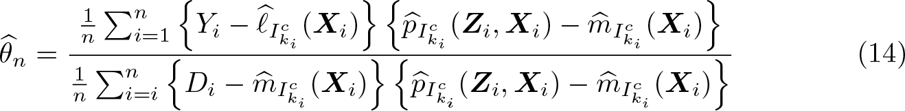
The DDML estimator based on the moment solution (13) is given by

${\widehat{\theta }}_n = \frac{\frac{1}{n} {\displaystyle {\sum }_{i=1}^n\left\{Y_i - {\widehat{\mathcal{l}}}_{I_{k_i}^c}\left({\mathit{X}}_i\right)\right\}}\left\{{\widehat{p}}_{I_{k_i}^c}\left({\mathit{Z}}_i,{\mathit{X}}_i\right) - {\widehat{m}}_{I_{k_i}^c}\left({\mathit{X}}_i\right)\right\}}{\frac{1}{n}{\displaystyle {\sum }_{i=i}^n\left\{D_i - {\widehat{m}}_{I_{k_i}^c}\left({\mathit{X}}_i\right)\right\}}\left\{{\widehat{p}}_{I_{k_i}^c}\left({\mathit{Z}}_i,{\mathit{X}}_i\right) - {\widehat{m}}_{I_{k_i}^c}\left({\mathit{X}}_i\right)\right\}}$

14

where ${\widehat{\mathcal{l}}}_{I_k^c} , {\widehat{m}}_{I_k^c},$ and ${\widehat{p}}_{I_k^c}$ are appropriate cross-fitted CEF estimators.

In simulations, we find that the finite-sample performance of the estimator in (14) improves when the LIE applied to E{p ₀( Z , X )} = m ₀( X ) is explicitly approximately enforced in estimation. As a result, we propose an intermediate step to the previously considered two-step DDML algorithm: Rather than estimating the conditional expectation of D given X directly, we estimate it by projecting first-step estimates of the conditional expectation of p ₀( Z , X ) onto X instead. Algorithm 2 outlines the LIE-compliant DDML algorithm for computation of (14).

Algorithm 2: LIE-compliant DDML for the flexible partially linear IV model

Split the sample ${\left\{\left(Y_i,D_i,{\mathit{X}}_i,{\mathit{Z}}_i\right)\right\}}_{i=1}^n$ randomly in K folds of approximately equal size. Denote I_k the set of observations included in fold k and $I_k^c$ its complement.

1. For each k ∊ {1,…, K}, do the following:

Fit a CEF estimator to the subsample $I_k^c$ using Y_i as the outcome and X _i as predictors. Obtain the out-of-sample predicted values ${\widehat{\mathcal{l}}}_{I_k^c}({\mathit{X}}_i)$ for i ∊ I_k .

Fit a CEF estimator to the subsample $I_k^c$ using D_i as the outcome and ( Z _i, X _i ) as predictors. Obtain the out-of-sample predicted values ${\widehat{p}}_{I_k^c}\left({\mathit{Z}}_i,{\mathit{X}}_i\right)$ for i ∊ I_k and in-sample predicted values ${\widehat{p}}_{I_k^c}\left({\mathit{Z}}_i,{\mathit{X}}_i\right)$ for i ∊ $I_k^c$ .

Fit a CEF estimator to the subsample $I_k^c$ using the in-sample predicted values ${\widehat{p}}_{I_k^c}\left({\mathit{Z}}_i,{\mathit{X}}_i\right)$ as the outcome and X _i as predictors. Obtain the out-of-sample predicted values ${\widehat{m}}_{I_k^c}({\mathit{X}}_i)$ for i ∊ I_k .

2. Compute (14).

Standard errors corresponding to ${\widehat{\theta }}_n$ in (14) are the same as in section 3.1, where the instrument is now given by ${\widehat{p}}_{I_{k_i}^c}\left({\mathit{Z}}_i,{\mathit{X}}_i\right)-{\widehat{m}}_{I_{k_i}^c}\left({\mathit{X}}_i\right)$ . Mean and median aggregation over cross-fitting repetitions are as outlined in remark 2.

3.3 Interactive IV model (interactiveiv)

The interactive IV model considers the same causal model as in section 2.2; specifically,

$Y=g_0(D,\mathit{X}) +U$

where D takes values in {0, 1}. The key difference from the interactive model is that this section considers identification via a binary instrument Z representing assignment to treatment.

The parameter of interest we target is

${\theta }_0=E\{g_0(1,\mathit{X})-g_0(0,\mathit{X})|p_0(1,\mathit{X})> p_0(0,\mathit{X})\}$

where p ₀(Z, X ) ≡ Pr(D = 1|Z, X ). Here θ ₀ is a local average treatment effect (LATE). Note that in contrast to the LATE developed in Imbens and Angrist (1994), we follow the exposition in Chernozhukov et al. (2018), where “local” does not strictly refer to compliers but instead to observations with a higher propensity score—that is, a higher probability of complying. ¹⁴

Identification again leverages assumptions 6 and 7, made in the context of the flexible partially linear IV model. In addition, we assume that the propensity score is weakly monotone with probability 1 and that the support of the instrument is independent of the controls.

Assumption 8 (Monotonicity). p ₀(1, X ) ≥ p ₀(0, X ) with probability 1.

Assumption 9 (IV overlap). Pr(Z = 1| X ) ∊ (0, 1) with probability 1.

Assumptions 6–9 imply that

${\theta }_0 = \frac{E\left\{{\mathcal{l}}_0(1,\mathit{X}) - {\mathcal{l}}_0(0,\mathit{X})\right\}}{E\left\{p_0(1,\mathit{X}) - p_0(0,\mathit{X})\right\}}$

15

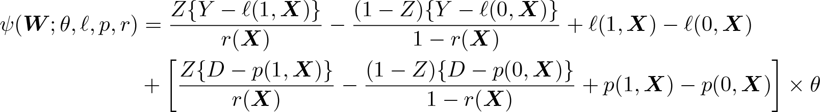
where ℓ ₀(Z, X ) ≡ E(Y|Z, X ), verifying identification of the LATE θ ₀. Akin to section 6, however, estimators of θ ₀ should not directly be based on (15) because the estimating equations implicit in obtaining (15) do not satisfy Neyman orthogonality. Hence, a direct estimator of θ ₀ obtained by plugging nonparametric estimators in for nuisance functions in (15) will potentially be highly sensitive to the first-step nonparametric estimation error. Rather, we base estimation on the Neyman orthogonal score function

$\begin{array}{l}\psi (\mathit{W};\theta ,\mathcal{l},p,r)\hspace{0.17em} =\hspace{0.17em} \frac{Z\{Y-\mathcal{l}(1,\mathit{X})\}}{r(\mathit{X})} - \frac{(1-Z)\{Y-\mathcal{l}(0,\mathit{X})\}}{1-r(\mathit{X})} + \mathcal{l}(1,\mathit{X}) - \mathcal{l}(0,\mathit{X})\\ + \left[\frac{Z\{D -p(1,\mathit{X})\}}{r(\mathit{X})}-\frac{(1-Z)\{D - p(0,\mathit{X})\}}{1 - r(\mathit{X})}\hspace{0.17em} + p(1,\mathit{X}) - p(0,\mathit{X})\right]\hspace{0.17em}\times \hspace{0.17em}\theta \end{array}$

where W ≡ (Y, D, X , Z). Note under assumptions 6–9 and for ℓ ₀(Z, X ) ≡ E(Y|Z, X ), p ₀(Z, X ) ≡ E(D|Z, X ), and r ₀( X ) ≡ E(Z| X ), we have E{ψ( W ; θ ₀ , ℓ ₀ , p ₀ , r ₀)} = 0 and can verify that its Gateaux derivative with respect to the nuisance functions local to their true values is also zero.

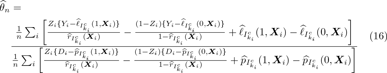
The DDML estimator based on the orthogonal score ψ is then

${\widehat{\theta }}_n\hspace{0.17em}=\hspace{0.17em}\frac{\frac{1}{n}{\displaystyle {\sum }_i\left[\frac{Z_i\left\{Y_i-{\widehat{\mathcal{l}}}_{I_{k_i^c}^c}\left(1,{\mathit{X}}_i\right)\right\}}{{\widehat{r}}_{I_{k_i}^c}\left({\mathit{X}}_i\right)}-\frac{\left(1-Z_i\right)\left\{Y_i-{\widehat{\mathcal{l}}}_{I_{k_i}^c}\left(0,{\mathit{X}}_i\right)\right\}}{1-{\widehat{r}}_{I_{k_i}^c}\left({\mathit{X}}_i\right)}+{\widehat{\mathcal{l}}}_{I_{k_i}^c}\left(1,{\mathit{X}}_i\right) - {\widehat{\mathcal{l}}}_{I_{k_i}^c}\left(0,{\mathit{X}}_i\right)\right]}}{\frac{1}{n} {\displaystyle {\sum }_i\left[\frac{Z_i\left\{D_i-{\widehat{p}}_{I_{k_i}^c}\left(1,{\mathit{X}}_i\right)\right\}}{{\widehat{r}}_{I_{k_i}^c}\left({\mathit{X}}_i\right)} - \frac{\left(1-Z_i\right)\left\{D_i-{\widehat{p}}_{I_{k_i}^c}\left(0,{\mathit{X}}_i\right)\right\}}{1-{\widehat{r}}_{I_{k_i}^c}\left({\mathit{X}}_i\right)}+{\widehat{p}}_{I_{k_i}^c}\left(1,{\mathit{X}}_i\right)-{\widehat{p}}_{I_{k_i}^c}\left(0,{\mathit{X}}_i\right)\right]}}$

16

where ${\widehat{\mathcal{l}}}_{I_k^c}$ , ${\widehat{p}}_{I_k^c}$ , and ${\widehat{r}}_{I_k^c}$ are appropriate cross-fitted CEF estimators. Because Z is binary, the cross-fitted values ${\widehat{\mathcal{l}}}_{I_k^c} \left(1,\mathit{X}\right)$ and ${\widehat{p}}_{I_k^c} (1,\mathit{X})$ , as well as ${\widehat{\mathcal{l}}}_{I_k^c} \left(0,\mathit{X}\right)$ and ${\widehat{p}}_{I_k^c} (0,\mathit{X})$ , are computed by using only assigned and unassigned observations, respectively.

ddml supports heteroskedasticity and cluster–robust standard errors for ${\widehat{\theta }}_n$ . Mean and median aggregation over cross-fitting repetitions are implemented as outlined in remark 2.

4 The choice of machine learner

Chernozhukov et al. (2018) show that DDML estimators are asymptotically normal when used in combination with a general class of machine learners satisfying a relatively weak convergence-rate requirement for estimating the CEFs. While asymptotic properties of common machine learners remain a highly active research area, recent advances provide convergence rates for special instances of many machine learners, including lasso (Bickel, Ritov, and Tsybakov 2009; Belloni et al. 2012), random forests (Wager and Walther 2015; Wager and Athey 2018; Athey, Tibshirani, and Wager 2019), neural networks (Schmidt-Hieber 2020; Farrell, Liang, and Misra 2021), and boosting (Luo, Spindler, and Kück 2016). It seems likely that many popular learners will fall under the umbrella of suitable learners as theoretical results are further developed. However, we note that currently known asymptotic properties do not cover a wide range of learners, such as very deep and wide neural networks and deep random forests, as they are currently implemented in practice.

The relative robustness of DDML to the first-step learners leads to the question of which machine learner is the most appropriate for a given application. It is ex ante rarely obvious which learner will perform best. Further, rather than restricting ourselves to one learner, we might want to combine several learners into one final learner. This is the idea behind stacking generalization, or simply “stacking”, due to Wolpert (1992) and Breiman (1996). Stacking allows one to accommodate a diverse set of base learners with varying tuning and hypertuning parameters. It thus provides a convenient framework for combining and identifying suitable learners, thereby reducing the risk of misspecification. Ahrens et al. (2024) introduce short-stacking, which reduces the computational cost of pairing DDML and stacking drastically, and pooled stacking, which enforces common weights across cross-fitting folds.

We discuss stacking approaches to DDML estimation in section 4.1. Section 4.2 demonstrates the performance of DDML in combination with stacking approaches using a simulation.

4.1 DDML and stacking

Our discussion of stacking in the context of DDML focuses on the partially linear model in (2), but we highlight that DDML and stacking can be combined in the same way for all other models supported in ddml. Suppose we consider J machine learners, referred to as base learners, to estimate the CEFs ℓ ₀( X ) ≡ E(Y| X ) and m ₀( X ) ≡ E(D| X ). The set of base learners could, for example, include cross-validated lasso and ridge with alternative sets of predictors, gradient-boosted (GB) trees with varying tree depths, and feed-forward neural nets with varying numbers of hidden layers and neurons. Generally, we recommend considering a relatively large and diverse set of base learners and including some learners with alternative tuning parameters.

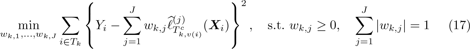
We randomly split the sample into K cross-fitting folds, denoted as I ₁ ,…, I_K . In each cross-fitting step k, we define the training sample as $I_k^c\equiv T_k$ , comprising all observations excluding the cross-fitting holdout fold k. This training sample is further divided into V cross-validation folds, denoted as T_{k, 1} ,…, T_k,V . The stacking regressor fits a final learner to the training sample T_k using the cross-validated predicted values of each base learner as inputs. A typical choice for the final learner is constrained least squares (CLS), which restricts the weights to be positive and sum to 1. The stacking objective function for estimating ℓ ₀( X ) using the training sample T_k is then defined as

$\underset{w_{k,1},\dots ,w_{k,J}}{ \min }\hspace{0.17em}{\displaystyle \sum _{i\in T_k}{\left\{Y_i - {\displaystyle \sum _{j=1}^J{w}_{k,j}}{\widehat{\mathcal{l}}}_{T_{k,v(i)}^c}^{(j)}\left({\mathit{X}}_i\right)\right\}}^2},\hspace{1em}\text{ s.t. }{w}_{k,j}\ge 0,\hspace{1em}{\displaystyle \sum _{j=1}^J|w_{k,j}|} = 1$

17

where w_k,j are referred to as stacking weights. We use ${\widehat{\mathcal{l}}}_{T_{k,v(i)}^c}^{(j)}\left({\mathit{X}}_i\right)$ to denote the crossvalidated predicted value for observation i, which is obtained from fitting learner j on the subsample $T_{k,v(i)}^c \equiv T_k\backslash T_{k,v(i)}$ , that is, the subsample excluding the fold v(i) into which observation i falls. The stacking predicted values are obtained as, ${\displaystyle {\sum }_j{\widehat{w}}_{{ }_{k,j}}}{\widehat{\mathcal{l}}}_k^{(j)}\left({\mathit{X}}_i\right)$ where each learner j is fit on the step-k training sample T_k . The objective function for estimating m ₀( X ) is defined accordingly.

CLS frequently performs well in practice and facilitates the interpretation of stacking as a weighted average of base learners (Hastie, Tibshirani, and Friedman 2009). However, it is not the only sensible choice of combining base learners. For example, stacking could instead select the single learner with the lowest quadratic loss by imposing the constraint w_k,j ∊ {0, 1} and ∑ _k,j w_k,j = 1. We refer to this choice as “single best” and include it in our simulation experiments. We implement stacking for DDML using pystacked (Ahrens, Hansen, and Schaffer 2023).

Pooled stacking

A variant of stacking specific to DDML is pooled stacking. Standard stacking fits the final learner K separate times, once in each cross-fitting step, yielding K separate sets of stacking weights ${\widehat{w}}_{k,j}$ for the J learners. With DDML pooled stacking, we can impose the additional constraint in (17) that the weights are the same across all cross-fitting folds, ${\widehat{w}}_{k,j}={\widehat{w}}_j,\forall k$ By returning one set of stacking weights, pooled stacking imposes an additional degree of regularization and facilitates interpretation but suffers from the same high computational cost as pairing DDML with (regular) stacking.

Short-stacking

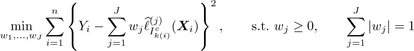
Stacking and pooled stacking rely on cross-validation. In the context of DDML, we can also exploit the cross-fitted predicted values directly for stacking. That is, we can directly apply CLS to the cross-fitted predicted values for estimating ℓ ₀( X ) [and similarly, m ₀( X )]:

$\underset{w_1,\dots ,w_J}{\min }{\displaystyle \sum _{i=1}^n{\left\{Y_i - {\displaystyle \sum _{j=1}^J{w}_j}{\widehat{\mathcal{l}}}_{I_{k(i)}^c}^{(j)}\left({\mathit{X}}_i\right)\right\}}^2},\hspace{1em}\text{ s.t. }{w}_j\ge 0,\hspace{1em}{\displaystyle \sum _{j=1}^J|w_j|} = 1$

We refer to this form of stacking that uses the cross-fitted predicted values as shortstacking because it takes a shortcut. This is to contrast it to regular stacking, which estimates the stacking weights for each cross-fitting fold k. The main advantage of short-stacking relative to standard stacking is the lower computational cost because short-stacking does not require the fitting of the j learners on subsamples to obtain the cross-validated predicted values ${\widehat{\mathcal{l}}}_{T_{k,v(i)}^c}^{(j)}\left({\mathit{X}}_i\right)$ needed for standard stacking. Furthermore, short-stacking (like pooled stacking) also produces one set of weights for the entire sample, which facilitates interpretation and implies a higher degree of regularization. A potential disadvantage of short-stacking is that it is more susceptible to overfitting issues because stacking weights and structural parameters are estimated using the same cross-fitted predicted values. We thus recommend only considering short-stacking in regular settings where the number of candidate learners is small relative to N (see also the discussion in Ahrens et al. [2024]). Algorithm A.4 in the online appendix summarizes the short-stacking algorithm for the partially linear model. ¹⁵

4.2 Monte Carlo simulation

To illustrate the advantages of DDML with stacking, we generate artificial data based on the partially linear model

$Y_i={\theta }_0{D}_i+c_{Y}g({\mathit{X}}_i) +{\sigma }_Y(D_i,{\mathit{X}}_i){\epsilon }_i$

18

$D_i=c_{D}g({\mathit{X}}_i) +{\sigma }_D({\mathit{X}}_i)u_i$

19

where both ε_i and u_i are independently drawn from the standard normal distribution. We set the target parameter to θ ₀ = 0.5 and the sample size to either n = 100 or n = 1000. The controls X _i are drawn from the multivariate normal distribution with N(0, Σ), where Σ _ij = (0.5)^{| i − j |}. The number of controls is set to p = dim( X _i ) = 50 except in DGP 5, where p = 7. The constants c_Y and c_D are chosen such that the R ² in (18) and (19) are approximately equal to 0.5. To induce heteroskedasticity, we set

${\sigma }_D\left({\mathit{X}}_i\right) = \sqrt{\frac{{\left\{1 + g\left({\mathit{X}}_i\right)\right\}}^2}{\frac{1}{n}{\displaystyle {\sum }_i{\left\{1 + g\left({\mathit{X}}_i\right)\right\}}^2}}}\hspace{1em}\text{ and }\hspace{1em}{\sigma }_Y\left(D_i,{\mathit{X}}_i\right) = \sqrt{\frac{{\left\{1 \hspace{0.17em}+ \hspace{0.17em}{\theta }_0{D}_i + g\left({\mathit{X}}_i\right)\right\}}^2}{\frac{1}{n}{\displaystyle {\sum }_i{\left\{1 + {\theta }_0{D}_i + g\left({\mathit{X}}_i\right)\right\}}^2}}}$

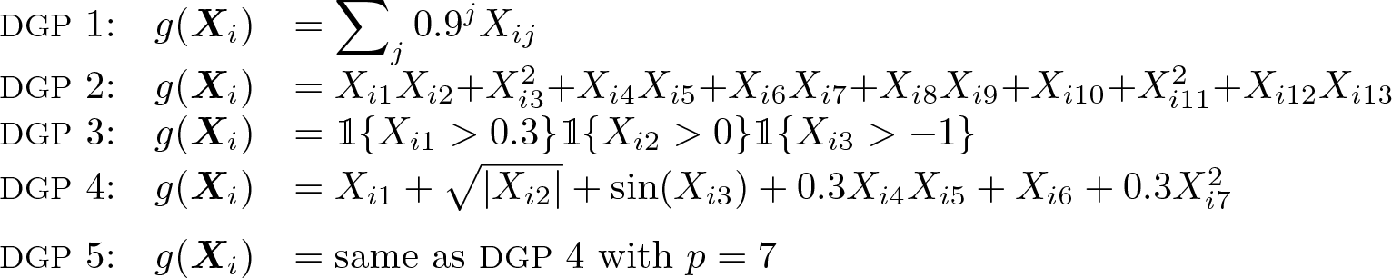
The nuisance function g( X _i ) is generated using five exemplary DGPs, which cover linear and nonlinear processes with varying degrees of sparsity and varying numbers of observed covariates:

$\begin{array}{l}\text{DGP} 1\hspace{0.17em}: \hspace{0.17em}g\left({\mathit{X}}_i\right) =\hspace{0.17em}{\displaystyle {\sum }_{j}0}{.9}^j{\mathit{X}}_{ij}\\ \text{DGP} 2\hspace{0.17em}:\hspace{0.17em}g\left({\mathit{X}}_i\right) ={\mathit{X}}_{i1}{\mathit{X}}_{i2} +{\mathit{X}}_{i3}^2 +{\mathit{X}}_{i4}{\mathit{X}}_{i5} +{\mathit{X}}_{i6}{\mathit{X}}_{i7} + {\mathit{X}}_{i8}{\mathit{X}}_{i9} + {\mathit{X}}_{i10} + {\mathit{X}}_{i11}^2 + {\mathit{X}}_{i12}{\mathit{X}}_{i13}\\ \text{DGP} 3\hspace{0.17em}:\hspace{0.17em}g\left({\mathit{X}}_i\right) =\mathbb{1}\left\{{\mathit{X}}_{i1}>0.3\right\}\mathbb{1}\left\{{\mathit{X}}_{i2}>0\right\}\mathbb{1}\left\{{\mathit{X}}_{i3}>-1\right\}\\ \text{DGP} 4\hspace{0.17em}:\hspace{0.17em}g\left({\mathit{X}}_i\right) ={\mathit{X}}_{i1} +\sqrt{|{\mathit{X}}_{i2}|} +\sin \left({\mathit{X}}_{i3}\right) +\hspace{0.17em} 0.3{\mathit{X}}_{i4}{\mathit{X}}_{i5} + {\mathit{X}}_{i6} +\hspace{0.17em}0.3{\mathit{X}}_{i7}^2\\ \text{DGP} 5\hspace{0.17em}:\hspace{0.17em}g\left({\mathit{X}}_i\right) =\text{same} \hspace{0.17em}\text{as} \hspace{0.17em} \text{DGP}\hspace{0.17em}\text{4} \hspace{0.17em} \text{with} p=\text{7}\end{array}$

DGP 1 is a linear design involving many negligibly small parameters. While not exactly sparse, the design can be approximated well through a sparse representation. DGP 2 is linear in the parameters and exactly sparse but includes interactions and secondorder polynomials. DGPs 3–5 are also exactly sparse but involve complex nonlinear and interaction effects. DGPs 4 and 5 are identical, except that DGP 5 does not add nuisance covariates that are unrelated to Y and D.

We consider DDML with the following supervised machine learners for cross-fitting the CEFs: ¹⁶

1.–2. Cross-validated lasso and ridge with untransformed base controls.

3.–4. Cross-validated lasso and ridge with fifth-order polynomials of base controls but no interactions (referred to as “Poly 5”).

5.–6. Cross-validated lasso and ridge with second-order polynomials and all first-order interaction terms (referred to as “Poly 2 + Inter.”).

7. Random forests with low regularization: base controls, maximum tree depth of 10, 500 trees, and approximately $\sqrt{p}$ features considered at each split.

8. Random forests with medium regularization: same as 7 but with maximum tree depth of 6.

9. Random forests with high regularization: same as 7 but with maximum tree depth of 2.

10. GB trees with low regularization: base controls, 1,000 trees, and a learning rate of 0.3. We enable early stopping, which uses a 20% validation sample to decide whether to stop the learning algorithm. Learning is terminated after five iterations with no meaningful improvement in the mean squared loss of the validation sample. ¹⁷

11. GB with medium regularization: same as 10 but with learning rate of 0.1.

12. GB with high regularization: same as 10 but with learning rate of 0.01.

13. Feed-forward neural net with base controls and 2 layers of size 20.

We use the above set of learners as base learners for DDML with stacking approaches. Specifically, we estimate DDML using stacking, short-stacking, and pooled stacking, which we combine with CLS and the single-best learner. We set the number of folds to K = 20 if n = 100 and to K = 5 if n = 1000. That is, we adapt the number of folds K to the total sample size n to ensure that the CEF estimators are trained on sufficiently large training samples.

For comparison, we report results for ordinary least squares (OLS) and PDS-lasso with base controls, PDS-lasso with Poly 5, PDS-lasso with Poly 2 + interactions, and an oracle estimator using the full sample. ¹⁸ The oracle estimator presumes knowledge of the function g( X ) and obtains estimates by regressing Y on the two variables D and g( X ).

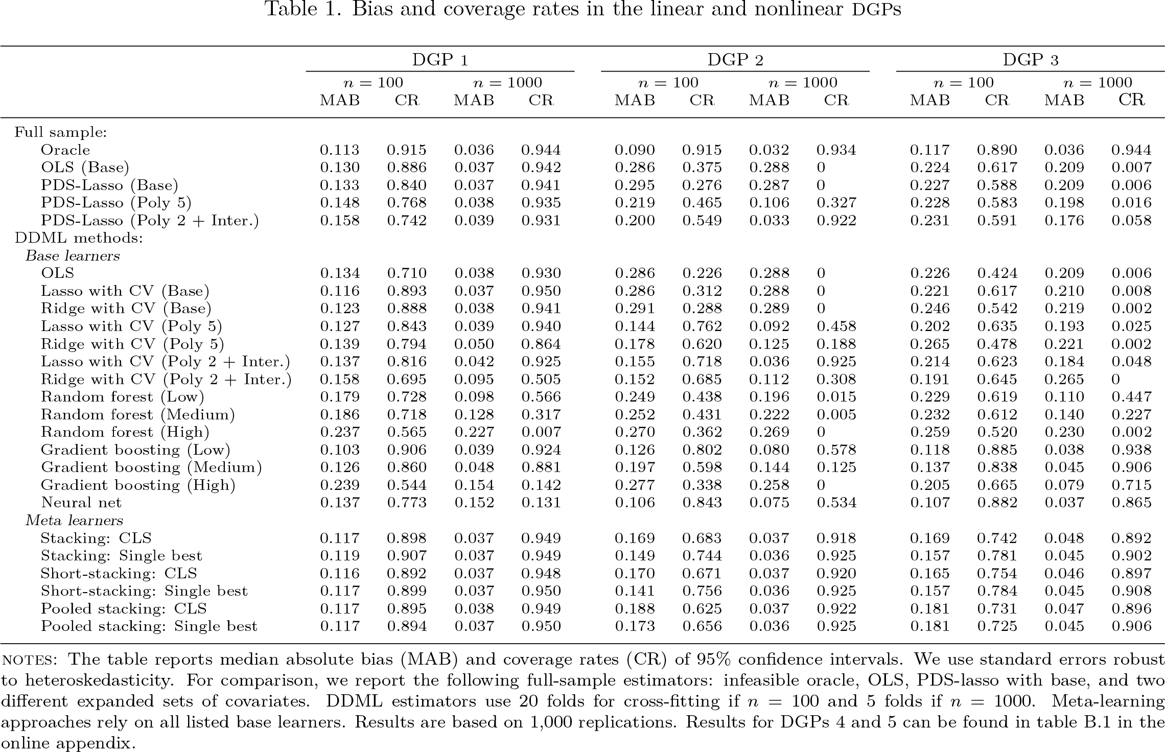
We report simulation median absolute bias (MAB) and coverage rates (CR) of 95% confidence intervals for DGPs 1–3 in table 1. We delegate results for DGPs 4 and 5, including a brief discussion, to online appendix B. DDML estimators leveraging stacking approaches perform favorably compared with individual base learners in terms of bias and coverage. The relative performance of stacking approaches seems to improve as the sample size increases, likely reflecting that the stacking weights are more precisely estimated in larger small samples. For n = 1000, the bias of stacking with CLS is at least as low as the bias of the best-performing individual learner under DGP 1–2, while only gradient boosting and neural net yield a lower bias than stacking under DGP 3.

Table 1.

Bias and coverage rates in the linear and nonlinear DGPs

	DGP 1				DGP 2				DGP 3
	n = 100		n = 1000		n = 100		n = 1000		n = 100		n = 1000
	MAB	CR	MAB	CR	MAB	CR	MAB	CR	MAB	CR	MAB	CR
Full sample:
Oracle	0.113	0.915	0.036	0.944	0.090	0.915	0.032	0.934	0.117	0.890	0.036	0.944
OLS (Base)	0.130	0.886	0.037	0.942	0.286	0.375	0.288	0	0.224	0.617	0.209	0.007
PDS-Lasso (Base)	0.133	0.840	0.037	0.941	0.295	0.276	0.287	0	0.227	0.588	0.209	0.006
PDS-Lasso (Poly 5)	0.148	0.768	0.038	0.935	0.219	0.465	0.106	0.327	0.228	0.583	0.198	0.016
PDS-Lasso (Poly 2 + Inter.)	0.158	0.742	0.039	0.931	0.200	0.549	0.033	0.922	0.231	0.591	0.176	0.058
DDML methods:
Base learners
OLS	0.134	0.710	0.038	0.930	0.286	0.226	0.288	0	0.226	0.424	0.209	0.006
Lasso with CV (Base)	0.116	0.893	0.037	0.950	0.286	0.312	0.288	0	0.221	0.617	0.210	0.008
Ridge with CV (Base)	0.123	0.888	0.038	0.941	0.291	0.288	0.289	0	0.246	0.542	0.219	0.002
Lasso with CV (Poly 5)	0.127	0.843	0.039	0.940	0.144	0.762	0.092	0.458	0.202	0.635	0.193	0.025
Ridge with CV (Poly 5)	0.139	0.794	0.050	0.864	0.178	0.620	0.125	0.188	0.265	0.478	0.221	0.002
Lasso with CV (Poly 2 + Inter.)	0.137	0.816	0.042	0.925	0.155	0.718	0.036	0.925	0.214	0.623	0.184	0.048
Ridge with CV (Poly 2 + Inter.)	0.158	0.695	0.095	0.505	0.152	0.685	0.112	0.308	0.191	0.645	0.265	0
Random forest (Low)	0.179	0.728	0.098	0.566	0.249	0.438	0.196	0.015	0.229	0.619	0.110	0.447
Random forest (Medium)	0.186	0.718	0.128	0.317	0.252	0.431	0.222	0.005	0.232	0.612	0.140	0.227
Random forest (High)	0.237	0.565	0.227	0.007	0.270	0.362	0.269	0	0.259	0.520	0.230	0.002
Gradient boosting (Low)	0.103	0.906	0.039	0.924	0.126	0.802	0.080	0.578	0.118	0.885	0.038	0.938
Gradient boosting (Medium)	0.126	0.860	0.048	0.881	0.197	0.598	0.144	0.125	0.137	0.838	0.045	0.906
Gradient boosting (High)	0.239	0.544	0.154	0.142	0.277	0.338	0.258	0	0.205	0.665	0.079	0.715
Neural net	0.137	0.773	0.152	0.131	0.106	0.843	0.075	0.534	0.107	0.882	0.037	0.865
Meta learners
Stacking: CLS	0.117	0.898	0.037	0.949	0.169	0.683	0.037	0.918	0.169	0.742	0.048	0.892
Stacking: Single best	0.119	0.907	0.037	0.949	0.149	0.744	0.036	0.925	0.157	0.781	0.045	0.902
Short-stacking: CLS	0.116	0.892	0.037	0.948	0.170	0.671	0.037	0.920	0.165	0.754	0.046	0.897
Short-stacking: Single best	0.117	0.899	0.037	0.950	0.141	0.756	0.036	0.925	0.157	0.784	0.045	0.908
Pooled stacking: CLS	0.117	0.895	0.038	0.949	0.188	0.625	0.037	0.922	0.181	0.731	0.047	0.896
Pooled stacking: Single best	0.117	0.894	0.037	0.950	0.173	0.656	0.036	0.925	0.181	0.725	0.045	0.906

NOTES: The table reports median absolute bias (MAB) and coverage rates (CR) of 95% confidence intervals. We use standard errors robust to heteroskedasticity. For comparison, we report the following full-sample estimators: infeasible oracle, OLS, PDS-lasso with base, and two different expanded sets of covariates. DDML estimators use 20 folds for cross-fitting if n = 100 and 5 folds if n = 1000. Meta-learning approaches rely on all listed base learners. Results are based on 1,000 replications. Results for DGPs 4 and 5 can be found in table B.1 in the online appendix.

Results for coverage are similar with stacking-based estimates being comparable with the best-performing feasible estimates and the oracle when n = 1000. With n = 100, coverage of confidence intervals for stacking-based estimators are inferior to coverages for a few of the individual learners but are still competitive and superior to most learners. Looking across all results, we see that stacking provides robustness to potentially very bad performance that could be obtained from using one poorly performing learner.

There are overall small performance differences among the six stacking estimators considered, suggesting that short-stacking has a substantial practical advantage because of its lower computational cost. Ahrens et al. (2024) report that short-stacking reduces the compute time by a factor of 1/V , where V is the number of cross-validation folds. There is some evidence that the single-best selector outperforms CLS in very small sample sizes in DGPs 2–3 but not in DGP 1 (and also not in DGPs 4–5; see table B.1). We suspect that the single-best selector works better in scenarios where there is one base learner that clearly dominates.

The mean squared prediction errors (MSPE) and the average stacking weights, which we report in tables B.2 and B.3 in the online appendix, provide further insights into how stacking functions with CLS. CLS assigns large stacking weights to base learners with low MSPEs, which in turn are associated with low biases. Importantly, stacking assigns zero or close-to-zero weights to poorly specified base learners such as the highly regularized random forest, which in all three DGPs ranks among the individual learners with the highest MSPE and the highest bias. The robustness to misspecified and illchosen machine learners, which could lead to misleading inference, is indeed one of our main motivations for advocating stacking approaches to DDML.

DDML with stacking approaches also compares favorably with conventional fullsample estimators. In the relatively simple linear DGP 1, DDML with stacking performs similarly to OLS and the infeasible oracle estimator—both in terms of bias and coverage—for n = 100 and n = 1000. In the more challenging DGPs 2 and 3, the bias of DDML with stacking is substantially lower than the biases of OLS and the PDS-lasso estimators. While the bias and size distortions of DDML with stacking are still considerable in comparison with the infeasible oracle for n = 100, they are close to the oracle for n = 1000. The results overall highlight the flexibility of DDML with stacking to flexibly approximate a wide range of DGPs, provided a diverse set of base learners is chosen.

5 The program

In this section, we provide an overview of the ddml package. We introduce the syntax and workflow for the main programs in section 5.1. Section 5.2 lists the options. Section 5.3 covers the simplified one-line program qddml. We provide an overview of supported machine learning programs in section 5.4. Finally, section 5.5 adds a note on how to ensure replication with ddml. See the help files for all available commands and options.

5.1 Syntax: ddml

The ddml estimation proceeds in four steps.

Step 1: Initialize ddml and select model

ddml init model [if] [in] [, mname( name ) kfolds( integer ) fcluster( varname ) foldvar( varlist ) reps( integer ) tabfold]

where model selects between the partially linear model (partial), the interactive model (interactive), the partially linear IV model (iv), the flexible partially linear IV model (fiv), and the interactive IV model (interactiveiv). This step creates a persistent Mata object with the name provided by mname(), in which model specifications and estimation results will be stored. The default is mname(m0).

At this stage, the user-specified folds for cross-fitting can be set via integer-valued Stata variables (see foldvar()). By default, observations are randomly assigned to folds and kfolds() determines the number of folds (the default is 5). Cluster-randomized fold splitting is supported (see fcluster()). The user can also select the number of times to fully repeat the cross-fitting procedure (see reps()).

Step 2: Add supervised machine learners for estimating conditional expectations

In step 2, we select the machine learning programs for estimating CEFs.

ddml cond_exp [, mname( name ) vname( varname ) learner( name ) vtype( string ) predopt( string )] : command depvar vars , cmdopt

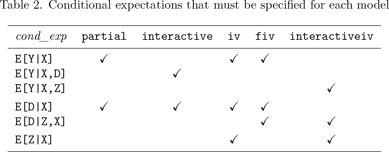
where cond_exp selects the conditional expectation to be estimated by the machine learning program command. At least one learner is required for each conditional expectation. Table 2 provides an overview of which conditional expectations are required by each model. The program command is a supervised machine learning program such as cvlasso or pystacked (see compatible programs in section 5.4). The options cmdopt are specific to that program.

Table 2.

Conditional expectations that must be specified for each model

cond_exp	partial	interactive	iv	fiv	interactiveiv
E[Y|X]	✔		✔	✔
E[Y|X,D]		✔
E[Y|X,Z]					✔
E[D|X]	✔	✔	✔	✔
E[D|Z,X]				✔	✔
E[Z|X]			✔		✔

Step 3: Perform cross-fitting

This step implements the cross-fitting algorithm. Each learner is fit iteratively on training folds, and out-of-sample predicted values are obtained. Cross-fitting is the most time-consuming step because it involves fitting the selected machine learners repeatedly.

ddml crossfit [, mname( name ) shortstack poolstack nostdstack finalest( name )]

Step 4: Estimate causal effects

Finally, we estimate the parameter of interest for all combinations of learners added in step 2.

ddml estimate [, mname( name ) robust cluster( varname ) vce( vcetype ) noconstant showconstant atet ateu trim( real ) shortstack poolstack finalest( name )]

To report and post selected results, we can use ddml estimate with the replay option:

ddml estimate [, mname( name ) spec( string ) rep( string ) allcombos notable replay]

Utilities

ddml describe provides information about the model setup or results:

ddml describe [, mname( name ) sample learners crossfit estimates all]

ddml stores many internal results on associate arrays, notably the various stacking weights. These can be retrieved using ddml extract:

ddml extract [ object_name , mname( name ) vname( varname ) ename( name ) stata show( display_item ) keys key1( string ) key2( string ) key3( string ) subkey1( string ) subkey2( string )]

ddml export saves the estimated conditional expectations and other variables to a CSV file:

ddml export filename [, mname( name ) addvars( varlist )]

5.2 Options

5.2.1 Step 1 options: Initialization

mname( name ) is the name of the DDML model. This option allows running of multiple DDML models simultaneously. The default is mname(m0).

kfolds( integer ) is the number of cross-fitting folds. The default is kfolds(5).

fcluster( varname ) is the cluster identifier for cluster randomization of folds.

foldvar( varlist ) is the integer variable to specify custom folds (one per cross-fitting repetition).

reps( integer ) is the number of cross-fitting repetitions, that is, how often the crossfitting procedure is repeated on randomly generated folds.

tabfold prints a table with frequency of observations by fold.

5.2.2 Step 2 options: Adding learners

vname( varname ) is the name of the dependent variable in the reduced-form estimation. This is usually inferred from the command line but is mandatory for the fiv model.

learner( name ) is the optional name of the variable to be created.

vtype( string ) is the optional variable type of the variable to be created. The default is vtype(double). none can be used to leave the type field blank. (Setting vtype(none) is required when using ddml with rforest.)

predopt( varname ) is the predict option to be used to get predicted values. Typical values could be xb or pr. The default is blank.

5.2.3 Step 3 options: Cross-fitting

shortstack asks for short-stacking to be used. Short-stacking uses the cross-fitted predicted values to obtain a weighted average of several base learners.

poolstack asks for pooled stacking to be used. This is available only if pystacked has been used for standard stacking in all equations.

nostdstack is used with pystacked and short-stacking; it tells pystacked to generate the base learner predictions without the computationally expensive additional step of obtaining the stacking weights.

finalest( name ) sets the final estimator for all stacking methods; the default estimator, finalest(nnls1), is least squares without a constant and with the constraints that weights are nonnegative and sum to 1. Alternative final estimators include singlebest (use the minimum mean squared error [MSE] base learner), ols (ordinary least squares), and avg (unweighted average of all base learners).

5.2.4 Step 4 options: Estimation

spec( string ) selects the specification. This can be either the specification number, mse for minimum-MSE specification (the default), or ss for short-stacking.

rep( string ) selects the cross-fitting repetitions. This can be the cross-fitting repetition number, mn for mean aggregation, or md for median aggregation (the default). See remark 2 for more information.

allcombos estimates all possible specifications. By default, only the minimum mean squared error, short-stacking, or pooled stacking specification is estimated and displayed.

notable suppresses the summary table.

replay is used in combination with spec() and rep() to display and return estimation results.

robust reports standard errors that are robust to the presence of arbitrary heteroskedasticity.

cluster( varname ) selects the cluster–robust variance–covariance estimator.

vce( vcetype ) selects the variance–covariance estimator, for example, vce(hc3) or vce(cluster id). See help regress##vcetype for available options.

noconstant suppresses the constant term in the estimation stage (only relevant for partially linear models).

showconstant displays the constant term in the summary estimation output table (partial, iv, and fiv models only).

atet reports the average treatment effect on the treated (the default is ATE).

ateu reports the average treatment effect on the untreated (the default is ATE).

trim( real ) trims propensity scores for the interactive and interactive IV models. The default is trim(0.01) (that is, values below 0.01 and above 0.99 are set to 0.01 and 0.99, respectively).

shortstack, poolstack, finalest( name ): see above under ddml crossfit.

Refitting the final learner using ddml estimate with stacking options is generally very fast because it does not require cross-fitting again.

For descriptions of the utility commands ddml describe, ddml extract, and ddml export and of their options, see their corresponding help files.

5.3 Short syntax: qddml

The ddml package includes the wrapper program qddml, which provides a one-line syntax for fitting a ddml model. The one-line syntax follows the syntax of pdslasso and ivlasso (Ahrens, Hansen, and Schaffer 2018). The main restriction of qddml compared with the more flexible multiline syntax is that qddml allows for only one user-specified machine learner.

qddml has integrated support for pystacked, which is the default learner in all equations. The syntax for qddml options differs depending on whether pystacked is used as the learner in each equation.

Syntax when used with pystacked

qddml depvar treatment_vars [( controls )] ( treatment_vars = excluded_instruments ), model( name ) [shortstack stdstack poolstack finalest( name ) pystacked( string ) pystacked_y( string ) pystacked_d( string ) pystacked_z( string ) options]

The pystacked() option sets the options for all the conditional expectations estimated by pystacked; the _y, _d, and _z variants control the options sent to the corresponding conditional expectation estimations. Other options are as in ddml.

Syntax when used with other learners

qddml depvar treatment_vars [( controls )] ( treatment_vars =excluded_instruments), model( name ) [cmd( string ) ycmd( string ) dcmd( string ) zcmd( string ) *cmdopt( string ) *vtype( name ) *predopt( name ) options]

The cmd() option sets the options for all the conditional expectations estimated by pystacked; the ycmd(), dcmd(), and zcmd() variants control the options sent to the corresponding conditional expectation estimations. The cmdopt() option can be used to either set the options for all equations or, if the asterisk is replaced with y, d, or z, set the options for the corresponding conditional expectation estimation. Other options are as in ddml.

5.4 Supported machine learning programs

ddml is compatible with any supervised machine learning program in Stata that supports the typical “regress y x” syntax, comes with a postestimation predict command, and supports if statements. We have tested ddml with the following programs:

pystacked facilitates the stacking of a wide range of machine learners, including regularized regression, random forests, support vector machines, GB trees, and feed-forward neural nets using Python’s scikit-learn (Ahrens, Hansen, and Schaffer 2023; Pedregosa et al. 2011; Buitinck et al. 2013). In addition, pystacked can also be used as a front-end to fit individual machine learners. ddml has integrated support for pystacked and is the recommended default learner.

lassopack implements regularized regression, for example, lasso, ridge, and elastic net (Ahrens, Hansen, and Schaffer 2020).

rforest is a random forest wrapper for Weka (Schonlau and Zou 2020; Frank et al. 2009).

svmachines allows for the estimation of support vector machines using libsvm (Chang and Lin 2011; Guenther and Schonlau 2018).

The program parsnip of the package mlrtime provides access to R’s parsnip machine learning library through rcall (Huntington-Klein 2021; Haghish 2019). Using parsnip requires the installation of the supplementary wrapper program parsnip2. ¹⁹

Stata programs that are currently not supported can be added relatively easily using wrapper programs (see parsnip2 for an example).

5.5 Inspecting results and replication

In this section, we discuss how to ensure replicability when using ddml. We also discuss some tools available for tracing replication failures. First, however, we briefly describe how ddml stores results.

ddml stores estimated conditional expectations in Stata’s memory as Stata variables. These variables can be inspected, graphed, and summarized as usual. Fold ID variables are also stored as Stata variables (named m0_fid_ r by default, where m0 is the default model name and r is the cross-fitting repetition). ddml models are stored on Mata structs and using Mata’s associative arrays. Specifically, the ddml model created by ddml init is an mStruct, and information relating to the estimation of conditional expectations is stored in eStructs. Results relating to the overall model estimation are stored in associative arrays that live in the mStruct, and results relating to the estimation of conditional expectations are stored in associative arrays that live in the corresponding eStructs.

Replication tips:

Set the Stata seed before ddml init. This ensures that the same random fold variable is used for a given dataset.

Using the same fold variable alone is usually not sufficient to ensure replication, because many machine learning algorithms involve randomization. That said, note that the fold variable is stored in memory and can be reused for subsequent estimations via the foldvar() option.

Replication of ddml results may require additional steps with some programs that rely on randomization in other software environments, for example, R or Python. pystacked uses a Python seed generated in Stata. Thus, when ddml is used with pystacked, setting the seed before ddml init also guarantees that the same Python seed underlies the stacking estimation. Other programs relying on randomization outside of Stata might not behave in the same way. Thus, when using other programs, check the help files for options to set external random seeds. Try estimating each individual learner on the entire sample to see what settings need to be passed to them for their results to replicate.

Beware of changing samples. Fold splits or learner idiosyncrasies may mean that sample sizes vary slightly across learners, estimation samples, or cross-fitting repetitions. ddml extract with the show(n) option will report sample sizes by learner and fold. See the ddml extract help file for more information.

The ddml export utility can be used to export the estimated conditional expectations, fold variables, and sample indicators to a CSV format file for examination and comparison in other software environments.

6 Applications

We demonstrate the ddml workflow using two applications. In section 6.1, we apply the DDML estimator to estimate the effect of 401(k) eligibility on financial wealth following Poterba, Venti, and Wise (1995). We focus on the partially linear model for the sake of brevity but provide code that demonstrates the use of ddml with the interactive model, partially linear IV model, and interactive IV model using the same application in online appendix C. Additional examples can also be found in the help file. Based on Berry, Levinsohn, and Pakes (1995), we show in section 6.2 how to use ddml for the estimation of the flexible partially linear IV model, which allows both for flexibly controlling for confounding factors using high-dimensional function approximation of confounding factors and for estimation of optimal IVs.

6.1 401(k) and financial wealth

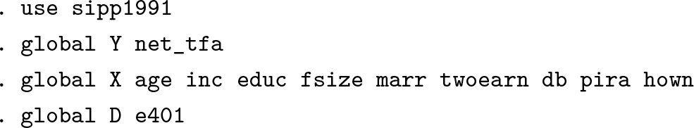
The data consist of n = 9915 households from the 1991 Survey of Income and Program Participation. The application is originally due to Poterba, Venti, and Wise (1995) but has been revisited by Belloni et al. (2017), Chernozhukov et al. (2018), and Wüthrich and Zhu (2023), among others. Following previous studies, we include the control variables age, income, years of education, and family size, as well as indicators for marital status, two-earner status, benefit pension status, individual retirement account participation, and home ownership. The outcome is net financial assets, and the treatment is eligibility to enroll for the 401(k) pension plan.

We load the data and define three globals for outcome, treatment, and control variables. We then proceed in the four steps outlined in section 5.1.

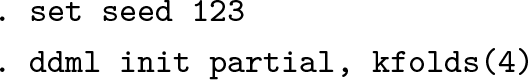
Step 1: Initialize ddml model

We initialize the ddml model and select the partially linear model in (2). Before initialization, we set the seed to ensure replication. This should always be done before ddml init, which executes the random fold assignment. In this example, we opt for four folds to ensure the readability of some of the output shown below, although we recommend considering more folds in practice.

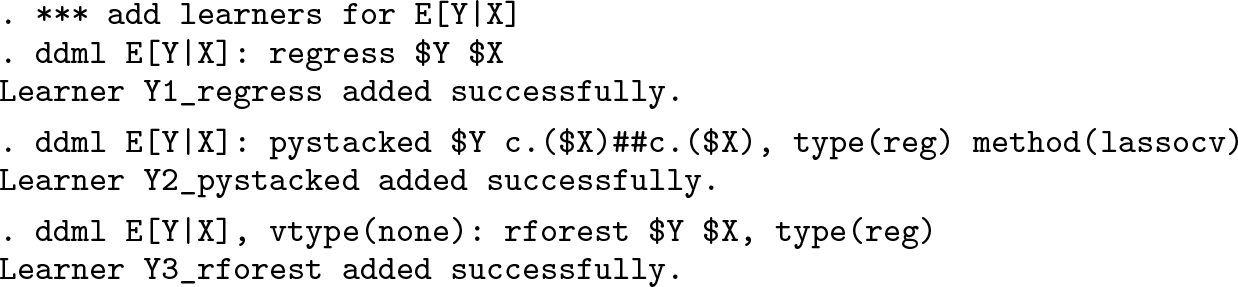
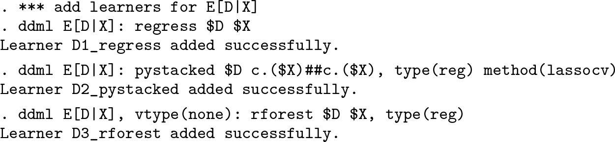
Step 2: Add supervised machine learners for estimating conditional expectations

In this step, we specify which machine learning programs should be used for the estimation of the conditional expectations E(Y | X ) and E(D| X ). For each conditional expectation, at least one learner is required. For illustrative purposes, we consider regress for linear regression, pystacked with the m(lassocv) option for cross-validated lasso (as an example of how to use pystacked to estimate one learner), and rforest for random forests. When using rforest, we need to add the option vtype(none) because the postestimation predict command of rforest does not support variable types.

The flexible ddml syntax allows specification of different sets of covariates for different learners. This flexibility can be useful because, for example, linear learners such as the lasso might perform better if interactions are provided as inputs, whereas tree-based methods such as random forests may detect certain interactions in a data-driven way. Here we use interactions and second-order polynomials for the cross-validated lasso but not for the other learners.

This application has only one treatment variable, but ddml does support multiple treatment variables. To add a second treatment variable, we would simply add a statement such as ddml E[D|X]: reg D2 $X, where D2 would be the name of the second treatment variable. An example with two treatments is provided in the help file.

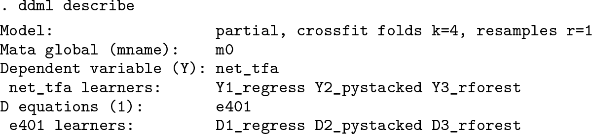
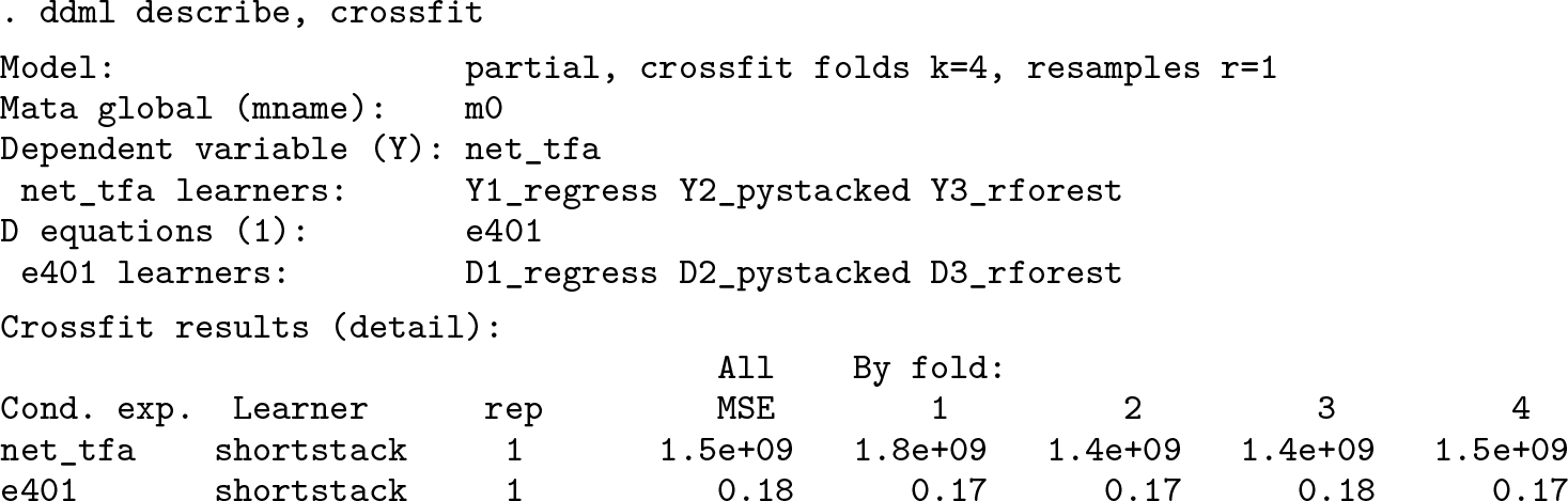
The auxiliary ddml subcommand describe allows us to verify that the learners were correctly registered:

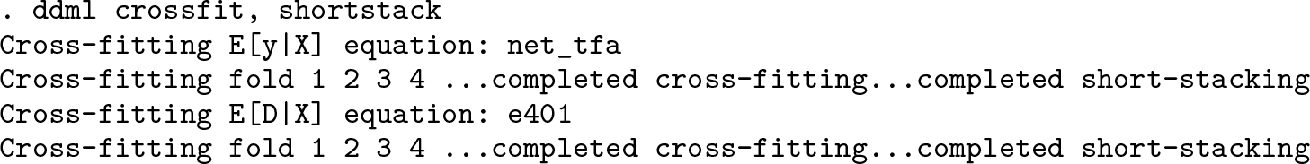
Step 3: Perform cross-fitting

The third step performs cross-fitting, which is the most time-intensive process. The shortstack option enables the short-stacking algorithm of section 4.1.

Six variables are created and stored in memory that correspond to the six learners specified in the previous step. These variables are called Y1_reg_1, Y2_pystacked_1_1, Y3_rforest_1, D1_reg_1, D2_pystacked_1_1, and D3_rforest_1. Y and D indicate the outcome and the treatment variable. Indexes 1 to 3 are learner counters. regress, pystacked, and rforest correspond to the names of the commands used. The _1 suffix indicates the cross-fitting repetition. The additional _1 in the case of D2_pystacked_1_1 indicates the learner number (there is only one pystacked learner).

After cross-fitting, we can inspect the mean squared prediction errors by fold and learner:

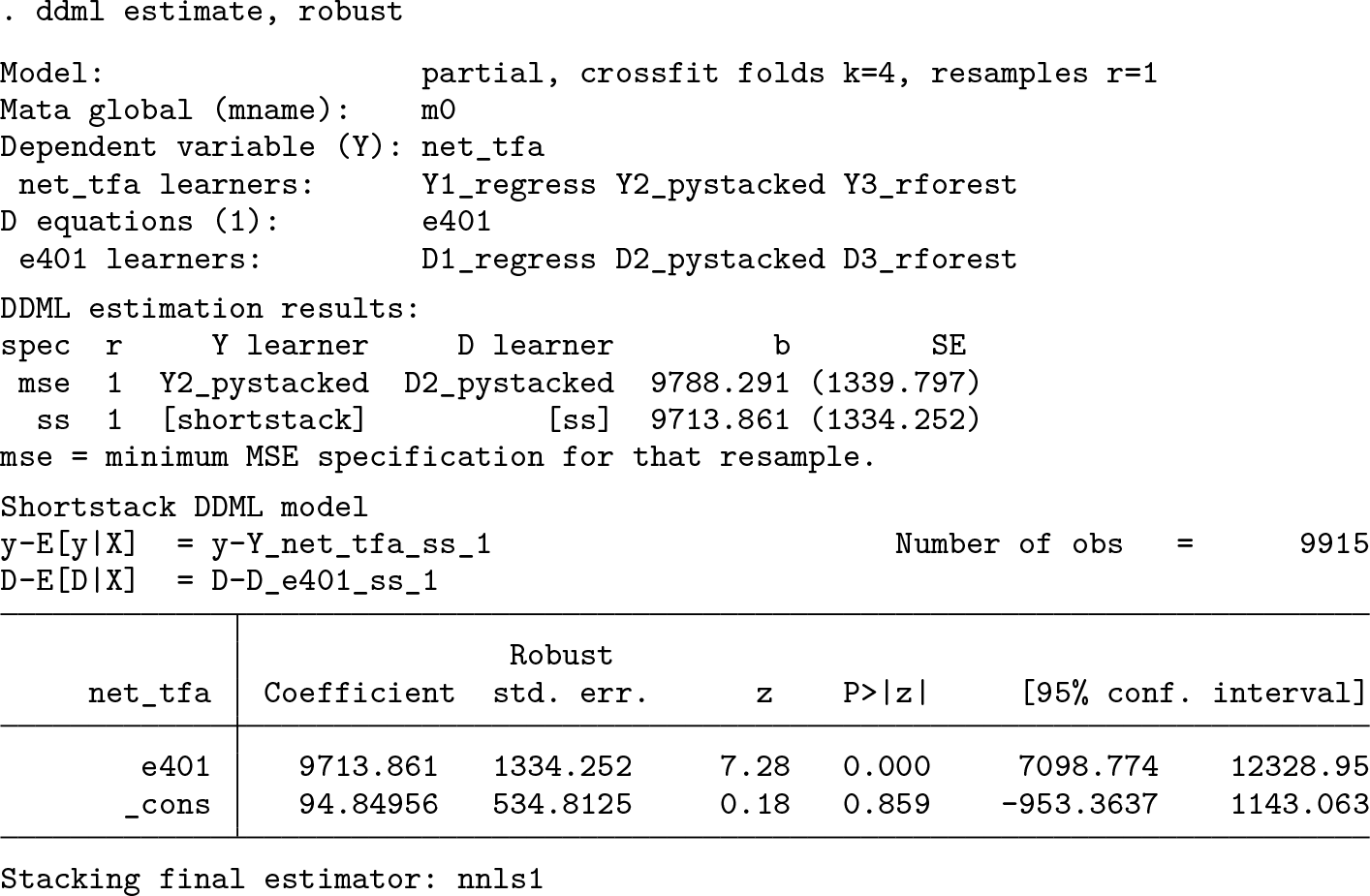
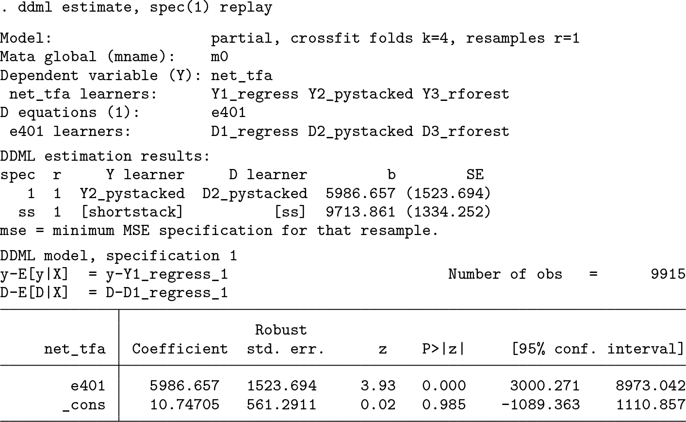
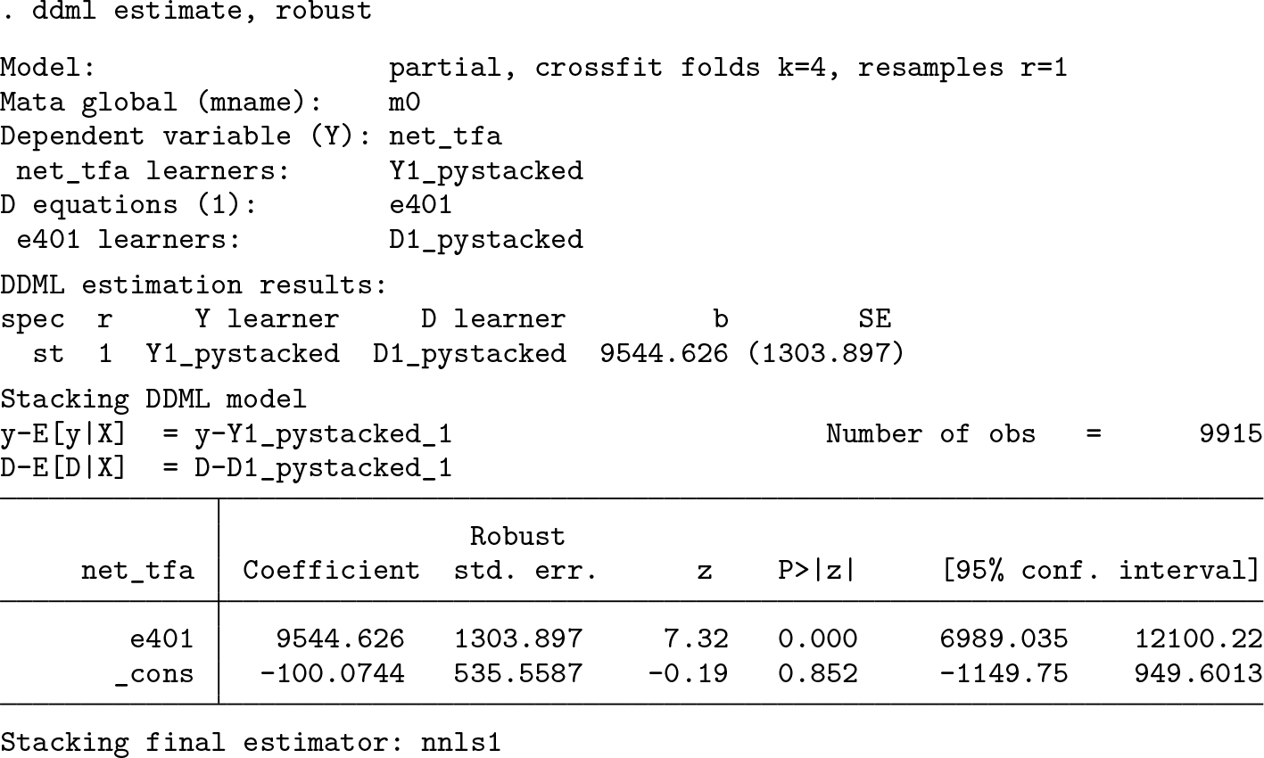
Step 4: Estimate causal effects

In this final step, we obtain the causal effect estimates. Because we requested shortstacking in step 3, ddml shows the short-stacking result, which relies on the crossfitted values of each base learner. In addition, the specification that corresponds to the minimum-MSE learners is listed at the beginning of the output.

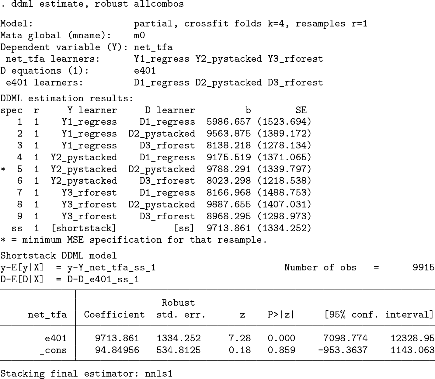
Because we have specified three learners per conditional expectation, there are nine specifications relying on the base learners in total (because we can combine Y1_reg_1, Y2_pystacked_1, and Y3_rforest_1 with D1_reg_1, D2_pystacked_1, and D3_rforest_1). To get all results, we add the allcombos option:

We can use the spec( string ) option to select among the listed specifications. string is either the specification number—ss, st, or ps to get the short-stacking, standard stacking, or pooled stacking specification, respectively—or mse for the specification corresponding to the minimal MSPE. In the example above, spec(1) reports in full the specification using regress for estimating both E(Y | X ) and E(D| X ). The spec() option can be provided either in combination with allcombos or after estimation in combination with the replay option, for example,

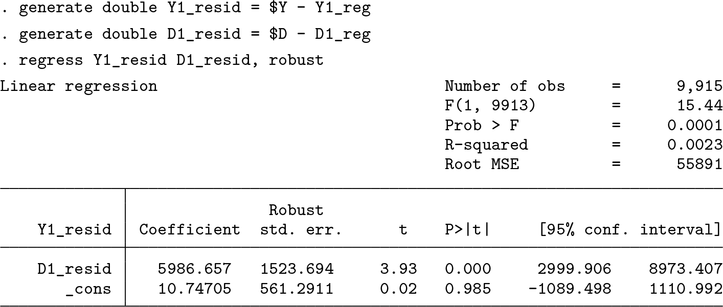
Manual final estimation

In the background, ddml estimate regresses Y1_reg_1 against D1_reg_1 with a constant. We can verify this manually:

Manual estimation using regress allows the use of regress’s postestimation tools.

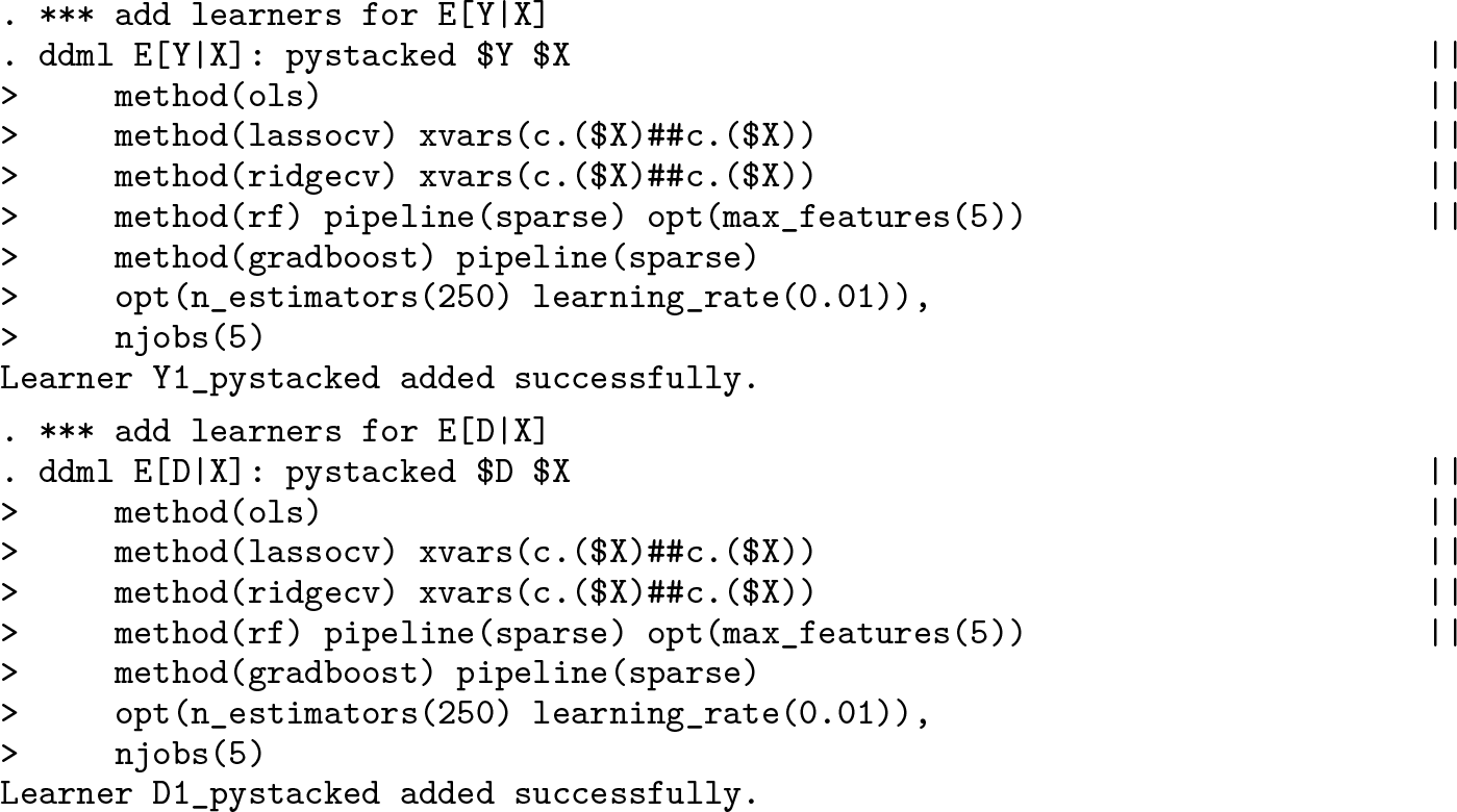
Stacking

We next demonstrate DDML with stacking. To this end, we exploit the stacking regressor implemented in pystacked. pystacked allows combining multiple base learners with learner-specific settings and covariates into a final meta-learner. The learners are separated by ||. method() selects the learner, xvars() specifies learner-specific covariates (overwriting the default covariates $X), and opt() passes options to the learners. In this example, we use OLS, cross-validated lasso and ridge, random forests, and gradient boosting. We furthermore use parallelization with five cores. A detailed explanation of the pystacked syntax can be found in Ahrens, Hansen, and Schaffer (2023).

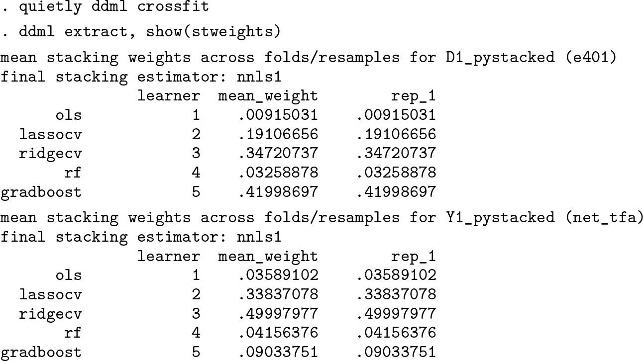
After cross-fitting, we retrieve the cross-fitted MSPE using the ddml extract command with show(mse) or examine the stacking weights using stweights:

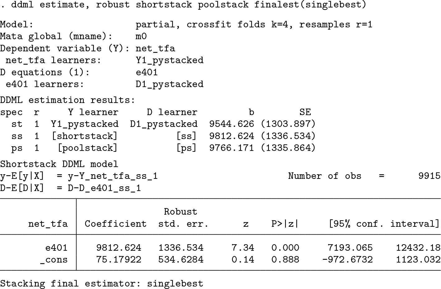
Finally, in the estimation stage, we retrieve the results of DDML with stacking:

The DDML-specific stacking approaches of short-stacking and pooled stacking can be requested at either the cross-fitting or the estimation step. Refitting the final learner at the estimation step allows us to avoid repeating the computationally intensive crossfitting. Here we request short-stacking and pooled stacking but using the single-best base learner.

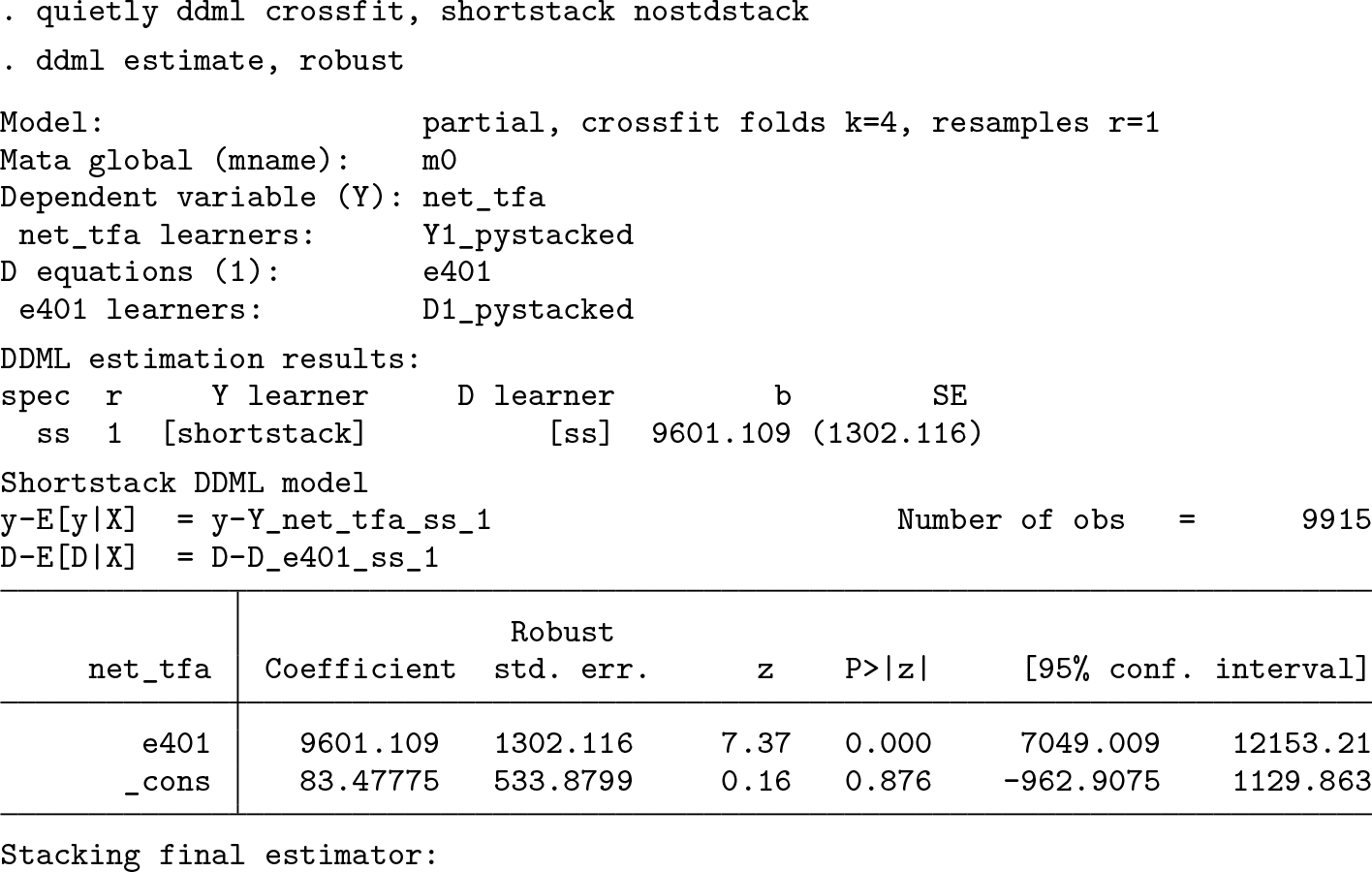
Short-stacking is computationally much faster than regular stacking (or pooled stacking) because it avoids the cross-validation within cross-fitting folds. Below, we disable regular stacking with the nostdstack option in the cross-fitting stage. In this example, where we use parallelization with 5 cores, the run time is only 50.7 seconds for DDML with short-stacking compared with 93.0 seconds for DDML with regular stacking.

One-line syntax

qddml provides a simplified and convenient one-line syntax. The main constraint of qddml is that it allows only for one user-specified learner. The default learner is pystacked, which by default uses OLS, cross-validated lasso, and gradient boosting as default learners. The pystacked base learners and non-pystacked commands can be modified via various options. Below, we use qddml with pystacked’s default base learners. We omit the output for the sake of brevity.

. quietly qddml $Y $D (c.($X)##c.($X)), model(partial) kfolds(4) robust

6.2 The market for automobiles

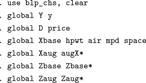
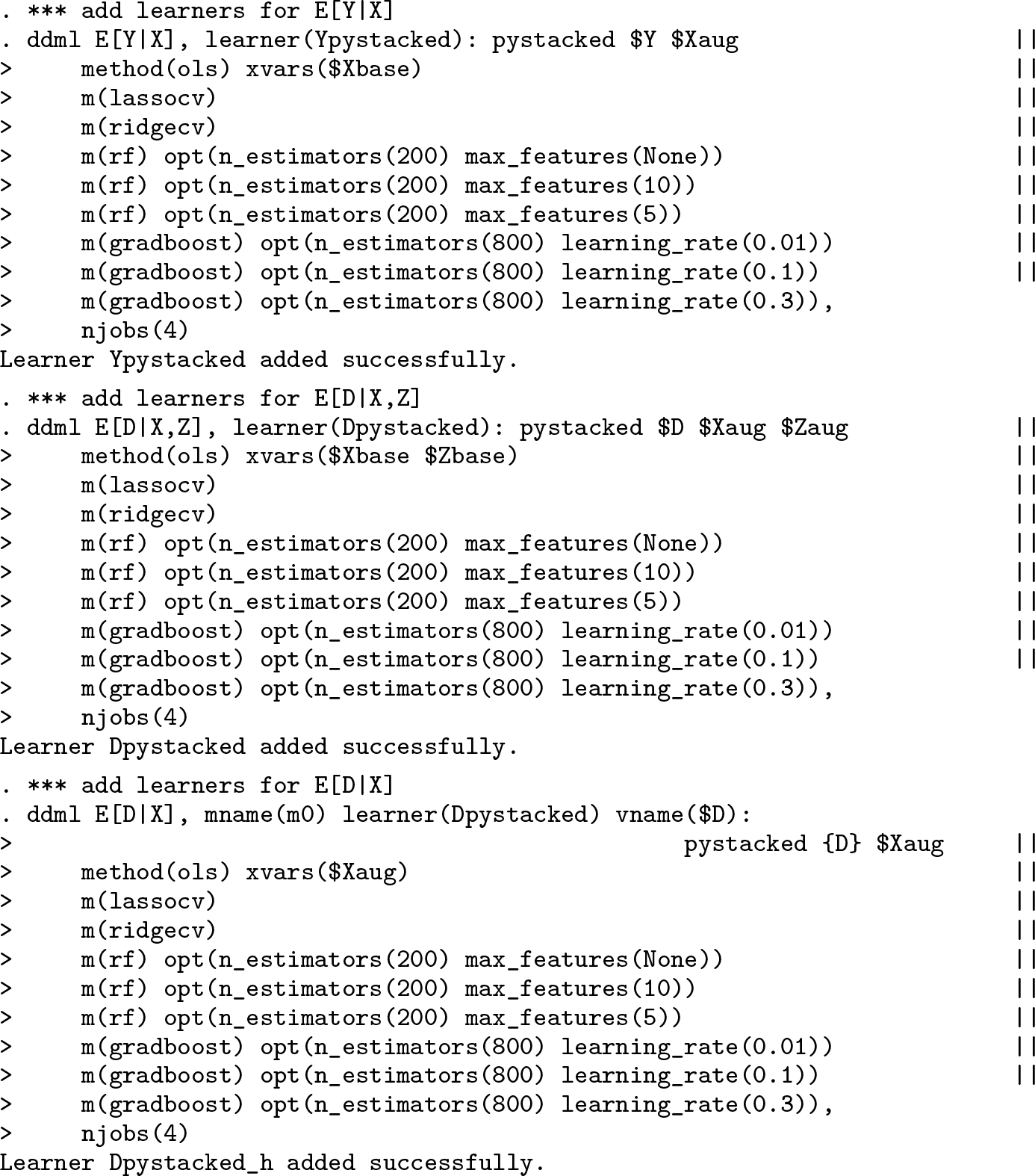
For this demonstration, we follow Chernozhukov, Hansen, and Spindler (2015b), who fit a stylized demand model using IVs based on the data from Berry, Levinsohn, and Pakes (1995). The authors of the original study estimate the effect of prices on the market share of automobile models in a given year (n = 2217). The controls are product characteristics (a constant, air conditioning dummy, horsepower divided by weight, miles per dollar, vehicle size). To account for endogenous prices, Berry, Levinsohn, and Pakes (1995) suggest exploiting other products’ characteristics as instruments. Following Chernozhukov, Hansen, and Spindler (2015b), we define the baseline set of instruments as the sum over all other products’ characteristics, calculated separately for own-firm and other-firm products, which yields 10 baseline instruments. Chernozhukov, Hansen, and Spindler (2015b) also construct an augmented set of instruments, including first-order interactions, squared terms, and cubic terms. In the analysis below, we extend Chernozhukov, Hansen, and Spindler (2015b) by applying DDML with stacking and a diverse set of learners, including OLS, lasso, ridge, random forest, and GB trees. We use the augmented set of controls for all base learners and OLS, which we include for reference.

We load and prepare the data:

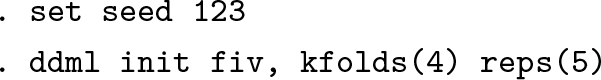
Step 1: Initialize ddml model

Note that in the ddml init step, we include the option reps(5), which will result in running the full cross-fitting procedure five times, each with a different random split of the data. Replicating the procedure multiple times allows us to gauge the impact of randomness due to the random splitting of the data into subsamples.

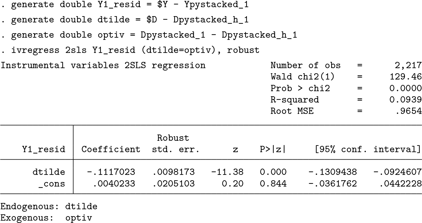
Step 2: Add supervised machine learners for estimating conditional expectations

Estimation of a fiv model requires us to add learners for E(Y | X ), E(D| X , Z ), and E(D| X ). Compared with the other models supported by ddml, there is one complication that arises because, to estimate E(D| X ), we exploit fitted values of E(D| X , Z ) to impose LIE compliance. Because these fitted values have not yet been generated, we use the placeholder {D}, which in the cross-fitting stage will be internally replaced with estimates of E(D| X , Z ). We use the learner() option to match one learner for E(D| X ) with a learner for E(D| X , Z ), and we use vname() to indicate the name of the treatment variable.

Steps 3–4: Perform cross-fitting (output omitted) and estimate causal effects

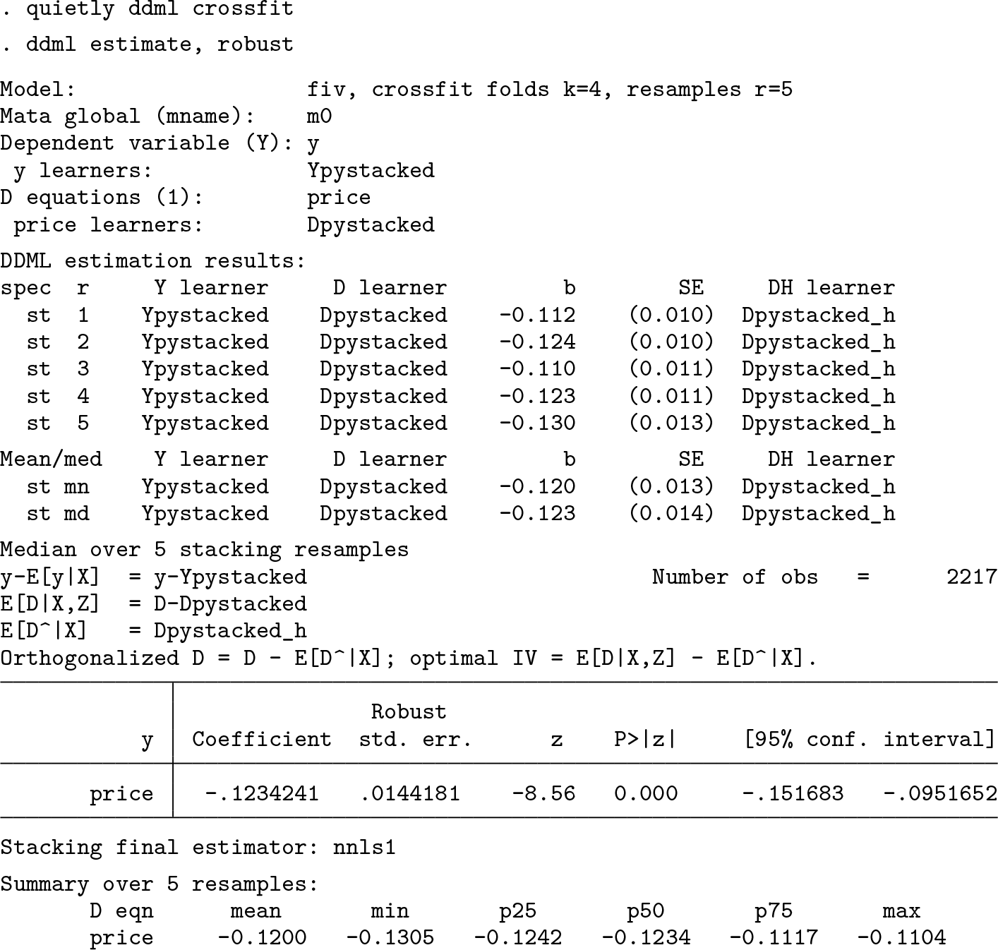
Manual final estimation

We can obtain the final estimate manually. To this end, we construct the instrument as $\widehat{E}(D\mid \mathit{X},Z)\hspace{0.17em}-\hspace{0.17em}\widehat{E}(D\mid \mathit{X})$ and the residualized endogenous regressor as $D\hspace{0.17em}-\hspace{0.17em}\widehat{E}(D\mid \mathit{X})$ . The residualized dependent variable is saved in memory. Here we obtain the estimate from the first cross-fitting replication. We could obtain the estimate for replication r by changing the “_1” to “_ r”.

7 Conclusion

This article introduced the command ddml, which implements double/debiased machine learning. It allows for flexible estimation of structural parameters in five econometric models, leveraging a wide range of supervised machine learners. While ddml is compatible with many existing machine learning programs in Stata, it is specifically designed to be used with pystacked, which allows combining several learners into a meta-learner via stacking. We see several avenues for extensions: First, ddml primarily focuses on crosssectional models. Some panel models are readily implementable in ddml, but expanding its capabilities for seamless use with a wide range of panel models would increase its practical relevance. Second, researchers and policymakers are frequently interested in learning treatment effects for specific subpopulations sharing observable characteristics. The estimation of conditional average treatment effects would be a natural extension to the existing ddml program. Third, ddml currently lacks underidentification diagnostics and weak-identification robust inference for IV regressions, which we hope to add in future releases.

9 Programs and supplemental material

Supplemental Material, sj-zip-1-stj-10.1177_1536867X241233641 - ddml: Double/debiased machine learning in Stata

Supplemental Material, sj-zip-1-stj-10.1177_1536867X241233641 for ddml: Double/debiased machine learning in Stata by Achim Ahrens, Christian B. Hansen, Mark E. Schaffer and Thomas Wiemann in The Stata Journal