Sage Journals: Discover world-class research

Abstract

We present a command, ardl, for the estimation of autoregressive distributed lag (ARDL) models in a time-series context. The ardl command can be used to fit an ARDL model with the optimal number of autoregressive and distributed lags based on the Akaike or Bayesian (Schwarz) information criterion. The regression results can be displayed in the ARDL levels form or in the error-correction representation of the model. The latter separates long-run and short-run effects and is available in two different parameterizations of the long-run (cointegrating) relationship. The popular bounds-testing procedure for the existence of a long-run levels relationship is implemented as a postestimation feature. Comprehensive critical values and approximate p-values obtained from response-surface regressions facilitate statistical inference.

Keywords

st0734 ardl ardl postestimation autoregressive distributed lag model error-correction model bounds test long-run relationship cointegration timeseries data

1 Introduction

Real-world phenomena are often characterized by complex relationships. Some observed variables might exhibit erratic behavior in the short run but tend to comove in a stable and predictable way over longer time horizons. Attempting to empirically uncover such long-run equilibrium relationships is tantamount to separating them from the overlaid short-run dynamics. This separation allows one to find evidence for or against an equilibrium relationship, which is often at the heart of a research question. It also allows analysis of the short-term fluctuations around the equilibrium, which can be valuable in its own right, for example, when conducting forecasting exercises or dynamic simulations.

When we observe the variables of interest over a sufficiently long stretch of consecutive time periods, multiequation vector autoregressive (VAR) and vector error-correction (VEC) models are commonly used to assess their dynamic relationships. When we have reasons to assume that there is a natural ordering of the variables such that there is no contemporaneous feedback from a response variable to the other variables in the system, a single-equation autoregressive distributed lag (ARDL) model can simplify the analysis and facilitate more efficient inference.¹

ARDL models have many possible applications. They are extensively used in studies analyzing linkages of pollution and energy consumption to economic growth (Fatai, Oxley, and Scrimgeour [2004]; Narayan and Smyth [2005]; Wolde-Rufael [2006]; Ang [2007]; Halicioglu [2009]; Jalil and Mahmud [2009]; Zhang et al. [2015]; Ntanos et al. [2018]; Bekun, Emir, and Sarkodie [2019]; Kirikkaleli, Güngör, and Adebayo [2022]; and many more). Relationships with economic growth have also been investigated for foreign direct investment and trade (Oteng-Abayie and Frimpong 2006; Belloumi 2014), infrastructure (Fedderke, Perkins, and Luiz 2006), immigration (Morley 2006), tourism (Katircioglu 2009; Wang 2009; Song et al. 2011), stock market development (Enisan and Olufisayo 2009), and health expenditures (Murthy and Okunade 2016).

Other examples include the nexus between viral infections and meteorological factors (He et al. 2017; Doğan et al. 2020), childcare availability, fertility, and female labor force participation (Lee and Lee 2014), wages, productivity, and unemployment (Pesaran, Shin, and Smith 2001), savings and investment (Narayan 2005), exchange rates and trade (Bahmani-Oskooee and Brooks 1999; De Vita and Abbott 2004), exchange rates and monetary policy (Frankel, Schmukler, and Servén 2004; Shambaugh 2004; Obstfeld, Shambaugh, and Taylor 2005), financial development and inequality (Ang 2010), bank lending and property prices (Davis and Zhu 2011), financial reforms and credit growth (Adeleye et al. 2018), stock market efficiency and fiscal policy (Stoian and Iorgulescu 2020), democracy and the shadow economy (Esaku 2022), and the interdependencies among stock price indices and commodity prices (Narayan, Smyth, and Nandha 2004; Sari, Hammoudeh, and Soytas 2010; Büyükşahin and Robe 2014), as well as cryptocurrencies (Ciaian, Rajcaniova, and Kancs 2016, 2018), to list only a few.

Recently, the ARDL methodological toolkit was used extensively to analyze adjustment processes during the COVID-19 pandemic, including tourism demand forecasts (Zhang et al. 2021) and the effects on macroeconomic activity (Varona and Gonzales 2021) or energy consumption (Aruga, Islam, and Jannat 2020).

The ARDL model can be conveniently reparameterized in so-called error-correction (EC) form, which disentangles the long-run relationship from the short-run dynamics. When the variables are nonstationary—to be precise, integrated of order 1—the longrun relationship embedded in an EC model corresponds to a cointegrating relationship (Engle and Granger 1987; Hassler and Wolters 2006). Testing for cointegration in such a setup therefore equals testing for the existence of a long-run relationship. However, the latter concept retains its relevance when some of or all the variables are stationary.

Pesaran and Shin (1998) and Hassler and Wolters (2006) highlight some advantages of the ARDL approach over alternative strategies for cointegration analysis—such as the Engle and Granger (1987) two-step procedure implemented in the community-contributed command egranger (Schaffer 2010) or the Phillips and Hansen (1990) fully modified ordinary least-squares approach implemented in cointreg (Wang 2012). First of all, it can accommodate a mixture of stationary and nonstationary variables without the need for pretesting the order of integration. Moreover, the short-run and long-run coefficients can be consistently estimated in one step, and the estimator’s asymptotic normality eases statistical inference.²

Compared with a system-based Johansen (1995) cointegration analysis, which is implemented in Stata’s vec command suite, the single-equation approach can be more efficient if the focus is on one outcome variable, in addition to the aforementioned flexibility regarding the integration orders. However, in the ARDL framework, the outcome variable is not allowed to simultaneously determine the long-run equilibrium of other explanatory variables, which would cause an endogeneity problem. The VAR or VEC approach can be more suitable for impulse–response analysis or dynamic forecasts because feedback from the dependent variable to the weakly exogenous variables is explicitly modeled.

Despite its advantages, testing for the existence of a long-run (cointegrating) relationship with the ARDL framework still requires a bit of effort. The test statistic has a nonstandard distribution that depends on various characteristics of the model and the data, including the integration order of the variables. Pesaran, Shin, and Smith (2001) propose a “bounds test”, which involves comparing the values of conventional F and t statistics with pairs of critical values (CV). Outside these bounds, the test either conclusively rejects or does not reject the null hypothesis. Within the bounds, the test is inconclusive.

This bounds test is implemented as a postestimation feature in our ardl package for the estimation of single-equation ARDL and EC models. Improved CV bounds and approximate p-values have been obtained by Kripfganz and Schneider (2020) with response-surface regressions using billions of simulated test statistics. These CVs are more precise and exhaustive than earlier ones tabulated by Pesaran, Shin, and Smith (2001) and Narayan (2005). A key feature of ardl is the automatic selection of the optimal lag order with the Akaike information criterion (AIC) or Bayesian (Schwarz) information criterion (BIC). With an increasing number of independent variables, the number of candidate models—which are characterized by all possible combinations of lag orders—is quickly in the tens or even hundreds of thousands. A computationally efficient implementation of this procedure ensures that the optimal model is still found within seconds.

Closely related, Jordan and Philips (2018) recently introduced the dynardl command for dynamic simulations of ARDL models. Their pssbounds command also provides an interface to display the original Pesaran, Shin, and Smith (2001) and Narayan (2005) asymptotic and finite-sample CVs for the bounds test. As argued above, those CVs are now largely superseded. Moreover, their commands do not perform an automatic lag-order selection, which is a key feature of our ardl command. Once the optimal model specification is obtained with the ardl command, the dynardl command can still be a useful complement if a visualization of the dynamic effects is desired.

This article is concerned only with time-series data. For the estimation of ARDL models in a large-T panel-data context, see the community-contributed commands xtpmg (Blackburne and Frank 2007), xtdcce2 (Ditzen 2018, 2021), and xtivdfreg (Kripfganz and Sarafidis 2021). The command xtwest (Persyn and Westerlund 2008) enables cointegration tests based on panel-data EC models.

In section 2, we outline the econometric background for the ARDL approach to the analysis of long-run equilibrium relationships, and we provide guidance for the model specification and bounds-testing procedure. In sections 3 and 4, we describe the syntax and options for the ardl package. In section 5, we illustrate the approach with an empirical example from the realm of cryptocurrencies. Section 5 concludes.

2 Econometric model and methods

2.1 ARDL model

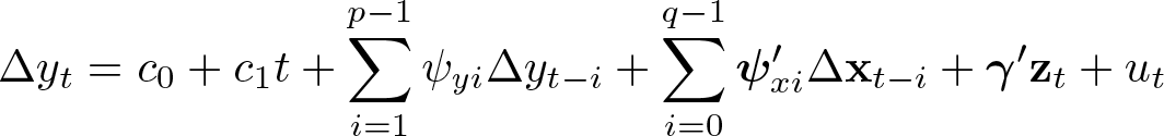
Suppose we expect the existence of an equilibrium relationship between an outcome variable y_t and a set of K explanatory variables x _t = (x ₁ _t, x ₂ _t,…, x_Kt )′:

y_{t} = b_{0} + b_{1} t + x_{t}^{'} θ + e_{t}

b ₀ is the intercept of the regression line, and b ₁ is the slope coefficient of a linear time trend. The data are observed at consecutive time points t = 1, 2,…, T . Estimating the regression coefficients in such a static model by ordinary least squares (OLS) might result in spuriously large coefficient estimates even if there is no underlying relationship among the variables. This is known to happen when the error term e_t is nonstationary because of the nonstationarity of y_t and x _t (after accounting for the possibility of a deterministic time trend).

Equation (1) remains a valid regression model if y_t and some of or all the variables x _t are cointegrated, that is, when y_t and x _t are individually integrated of order 1, I(1), but there exists a linear combination among them such that e_t is integrated of order 0, I(0). Equation (1) reflects a conditional long-run equilibrium relationship—if it exists—to which a process reverts over time. In the short run, the process might divert from this equilibrium, but the above equation is silent about the dynamic evolution of the process when it is off the equilibrium path. Such deviations are transitory, and the elements in the data-generating process (DGP) governing them are therefore I(0). These neglected I(0) components in the DGP affect the finite-sample (and possibly the asymptotic) distributions of test statistics and thus invalidate conventional hypothesis tests and regression diagnostics.³

To circumvent the problems associated with fitting a static model, we can augment the regression equation with lags of the dependent and independent variables. We can even include another set of L exogenous variables z _t , which may have predictive power to explain the short-term fluctuations of y_t but do not affect its equilibrium path. We assume that all variables in z _t are (trend) stationary. Augmenting the model in this way aims at obtaining a dynamically complete model in which the regression error term u_t is free of serial correlation:

y_{t} = c_{0} + c_{1} t + \sum_{i = 1}^{p} ϕ_{i} y_{t - i} + \sum_{i = 0}^{q} {β^{'}}_{i} x_{t - i} + γ^{'} z_{t} + u_{t}

t = 1 + p ^∗ ,…, T . Leaving aside the variables z _t , this is a general ARDL (p, q,…, q) model with intercept c ₀, linear trend c ₁ t, and lag orders p ∊ [1, p ^∗] and q ∊ [0, p ^∗].⁴ To ensure that there are enough degrees of freedom available to fit the model’s coefficients with sufficient precision, we may need to choose the maximum admissible lag order p ^∗ conservatively. This is especially relevant when the number of observations in the dataset (T ) is relatively small, the number of variables in x _t (K) is relatively large, or both.⁵

Given the initial observations y ₁ , y ₂ ,…, y_p ^∗ and the time paths of x _t and z _t , (2) describes the dynamic evolution of y_t over time, irrespective of whether an equilibrium relationship—as postulated in (1)—exists. The intercept c ₀ and the linear time trend c ₁ t may or may not be included in the model, depending on the nature of the variables under consideration.⁶ We assume that enough lags have been included in the ARDL model (2) to purge the error term from any remaining serial correlation and to ensure that the variables x _t are weakly exogenous/long-run forcing—ruling out any contemporaneous feedback from y_t to x _t . If there exists a stable long-run relationship, conventional asymptotic theory can be applied for statistical inference on any of the coefficients even if some of the variables are nonstationary (Pesaran and Shin 1998). This highlights the importance of testing for the existence of such a long-run relationship, which we consider in section 2.3.

While the inclusion of further lags improves the regression fit, this comes at the cost of a higher variance of the coefficient estimates. To balance this tradeoff, we can base a data-driven approach to optimal lag selection on the AIC or the BIC,

\begin{matrix} AIC = - 2 \ln (L) + 2 K^{*} \\ BIC = - 2 \ln (L) + \ln (T^{*}) K^{*} \end{matrix}

where $\ln (L)$ is the value of the log-likelihood function from the fitted regression model, T ^∗ = T − p ^∗ is the effective sample size, and K ^∗ = 2 + p + K(q + 1) + L is the number of estimated coefficients in (2). These criteria balance the desire for a better fit of the model—higher values of $\ln (L)$ —against the temptation of creating ever larger models. The BIC has a larger penalty term than the AIC (for T ^∗ ≥ 8) and therefore tends to select more parsimonious models. The optimal lag orders are then found by fitting model (2) for all possible combinations of p and q and choosing the model that minimizes the AIC or BIC.

For the comparability of the model-selection criteria, we must base all regressions on the same estimation sample. This is the reason for initially choosing a fixed maximum lag order p ^∗. When both p and q are smaller than p ^∗, the estimation of model (2) does not use all the available observations. This is the price we need to pay for consulting the model-selection criteria. Once the optimal lag orders p and q have been found, we can subsequently refit the model, utilizing all available observations by setting p ^∗ = max(p, q).

2.2 Error-correction representation

To gain a better interpretability of the model’s coefficients, we can reformulate the ARDL model in EC representation (Hassler and Wolters 2006):⁷

Δ y_{t} = c_{0} + c_{1} t - α (y_{t - 1} - θ x_{t - 1}) + \sum_{i = 1}^{p - 1} ψ_{y i} Δ y_{t - i} + ω^{'} Δ x_{t} + \sum_{i = 1}^{q - 1} ψ_{x i}^{'} Δ x_{t - i} + γ^{'} z_{t} + u_{t}

The coefficients in (3) can be mapped in a straightforward algebraic way to the coefficients in (2):

\begin{array}{l} α = 1 - \sum_{i = 1}^{p} ϕ_{i}, θ = \frac{\sum_{j = 0}^{q} β_{j}}{α} \\ ψ_{y i} = - \sum_{j = i + 1}^{p} ϕ_{j}, ω = β_{0}, ψ_{x i} = - \sum_{j = i + 1}^{q} β_{j} \end{array}

Now recall the hypothesized long-run equilibrium relationship between y_t and x _t in (1). Ignoring the intercept and linear time trend for the moment, we see the deviations from this equilibrium, e_t ₋ ₁ = y_t ₋ ₁ − θx _t ₋ ₁, can be found again in the EC model (3). Because of the nonlinear interaction between the coefficients α and θ , we cannot directly fit (3) with OLS. However, given the mapping above, we can recover consistent estimates of all coefficients from the ARDL model (2). Yet a computationally more convenient approach is to instead fit the following model:⁸

Δ y_{t} = c_{0} + c_{1} t + π_{y} y_{t - 1} + π_{x} x_{t - 1} + \sum_{i = 1}^{p - 1} ψ_{y i} Δ y_{t - i} + ω^{'} Δ x_{t} + \sum_{i = 1}^{q - 1} ψ_{x i}^{'} Δ x_{t - i} + γ^{'} z_{t} + u_{t}

From the above model, we can easily recover the so-called speed-of-adjustment coefficient α = −π_y and the long-run coefficients θ = π _x/α. The corresponding standard errors can be computed with the delta method (Pesaran and Shin 1998). Note that (4) collapses to the well-known augmented Dickey and Fuller (1979) regression for unit-root testing when no explanatory variables x _t and z _t are present (K = L = 0).

The speed-of-adjustment coefficient α tells us how fast the process for y_t reverts to its long-run relationship when this equilibrium is distorted. α = 1 would imply that—in the absence of any other short-run fluctuations—any deviation from the equilibrium is fully corrected immediately in the period after the distortion occurs. In contrast, α = 0 would imply that the process never returns to its equilibrium path. Values of α between these two boundaries reflect a partial-adjustment process, where the gap to the equilibrium is gradually closed over time.⁹

Clearly, θ ≠ 0 is not a sufficient condition for the existence of a conditional long-run relationship between the levels of y_t and x _t . When α = 0, then y_t is I(1) and no such relationship exists. In the opposite scenario, when θ = 0 and α ∊ (0, 2), then y_t is (trend) stationary, irrespective of the integration order of the components in x _t . For a long-run level relationship to exist, we need both θ ≠ 0 and α > 0. In this case—as long as the elements of x _t are not cointegrated among themselves—the integration properties of x _t determine the integration order of y_t . If the variables in x _t with nonzero long-run coefficient are I(1), then y_t is I(1) as well, and the conditional long-run relationship corresponds to a cointegrating relationship.

In this context, note that the assumption of x _t being long-run forcing for y_t implies that there can exist at most one cointegrating relationship that involves y_t . Consider the VEC model

(\begin{matrix} Δ y_{t} \\ Δ x_{t} \end{matrix}) = a_{0} + a_{1} t + (\begin{matrix} π_{y y} & π_{y x}^{'} \\ π_{x y} & Π_{x x} \end{matrix}) (\begin{matrix} y_{t - 1} \\ x_{t - 1} \end{matrix}) + \sum_{i = 1}^{p^{*} - 1} Ψ_{i} (\begin{matrix} Δ y_{t - i} \\ Δ x_{t - i} \end{matrix}) + Γ z_{t} + (\begin{matrix} ε_{y, t} \\ ε_{x, t} \end{matrix})

x _t is long-run forcing for y_t if it obeys the restriction π _xy = 0; that is, there is no level effect of y_t ₋ ₁ on Δx _t .¹⁰ This does not rule out further cointegrating relationships among the elements of x _t , Π _xx ≠ 0. Thus, without further inspection, a cointegration rank larger than one for the entire system ${(y_{t}, x_{t}^{'})}^{'}$ does not necessarily imply a violation of this assumption. However, if there is reason to suspect multiple cointegrating relationships involving y_t , π _xy ≠ 0, then a single-equation ARDL or EC model is inappropriate.¹¹ Instead, this would call for a multivariate cointegration analysis within the Johansen (1995) framework by fitting a VAR or VEC model.¹² In contrast, if π _xy = 0 is indeed satisfied and the interest is primarily on the long-run relationship between y_t and x _t , then fitting a single-equation model is more efficient and computationally straightforward.

The remaining coefficients ψ_yi , ω , ψ _xi , and γ in (3) capture the short-run dynamics that are not prescribed by the equilibrium-reverting forces.¹³ They not only are relevant for making dynamic forecasts but also play a role for choosing appropriate CVs when testing for the existence of a long-run relationship, which we explore in section 2.3.

A complication arises if q = 0 for some of or all the long-run forcing variables. In that situation, π _x = ω , which implies that the corresponding variance–covariance matrix of the coefficient estimates in (4) is rank deficient. To avoid this complication, we can equivalently formulate the EC representation with the levels of the long-run forcing variables expressed in period t instead of t − 1:

Δ y_{t} = c_{0} + c_{1} t - α (y_{t - 1} - θ x_{t}) + \sum_{i = 1}^{p - 1} ψ_{y i} Δ y_{t - i} + \sum_{i = 0}^{q - 1} ψ_{x i}^{'} Δ x_{t - i} + γ^{'} z_{t} + u_{t}

It has the same parameter restrictions as defined above. Note that ω ′Δx _t is replaced by $ψ_{x 0}^{'} Δ x_{t}$ . The interpretation of the long-run coefficients θ does not change because the time subscript does not matter when the process is in equilibrium. The equation to be estimated in this case becomes

Δ y_{t} = c_{0} + c_{1} t + π_{y} y_{t - 1} + π_{x} x_{t} + \sum_{i = 1}^{p - 1} ψ_{y i} Δ y_{t - i} + \sum_{i = 0}^{q - 1} ψ_{x i}^{'} Δ x_{t - i} + γ^{'} z_{t} + u_{t}

where the coefficients π _x are identical to the corresponding coefficients in (4), despite the change in the time subscript.¹⁴

2.3 Bounds test

Although we can consistently estimate all coefficients in the ARDL model (2) or its EC representations, testing for the existence of a long-run relationship involves a bit more effort. This is because the process for y_t contains a unit root under the null hypothesis of no long-run relationship; therefore, the test statistics have nonstandard distributions. Moreover, the tests depend on the choice of deterministic model components. In the ARDL model (2)—and its EC representations (3) and (6)—we have allowed for an intercept c ₀ and a linear time trend c ₁ t. We can distinguish the following five cases:

No deterministic model components are included (c ₀ = c ₁ = 0).

A restricted intercept is included (c ₀ = αb ₀) but no time trend (c ₁ = 0).

An unrestricted intercept is included (c ₀ ≠ 0) but no time trend (c ₁ = 0).

An unrestricted intercept is included (c ₀ ≠ 0) and a restricted time trend (c ₁ = αb ₁).

Both deterministic model components are unrestricted (c ₀ ≠ 0 and c ₁ ≠ 0).

A decision about the relevant case can often be guided by a visual inspection of the time series. Cases 1 and 2 are in line with a process y_t , which could reasonably be an I(1) process without drift under the null hypothesis of no long-run level relationship. Under the alternative hypothesis, y_t would either be I(0) or cointegrated with x _t . Case 1 is most appropriate if y_t and x _t fluctuate around a zero mean or if any nonzero means cancel out in the long-run level relationship; that is, b ₀ = b ₁ = 0 in (1). The latter condition is hard to verify ex ante, such that case 2 is often the safer option whenever some variables have a nonzero mean.

If y_t appears to be trending, it could be an I(1) process with drift under the null hypothesis. This calls for case 3 or 4. Under the alternative hypothesis, y_t would either be trend stationary or cointegrated with x _t . Case 3 is most appropriate if the trend in y_t is entirely attributable to a trend in x _t ; that is, b ₁ = 0 in (1). Again, this may be difficult to justify ex ante. Despite the fact that case 3 is most commonly applied in the empirical practice, case 4 is generally the safer option when there is insufficient knowledge about the source of the observed time trend.

Especially when the sample size is relatively small, it might be difficult to distinguish visually between a mildly drifting unit-root process under the null hypothesis and a stationary process which is fluctuating around a constant mean under the alternative hypothesis. This can be another relevant situation for case 3. Similarly, case 5 could be used to statistically discriminate between a unit-root process with faster—although hardly noticeable—than linear growth (or decline) and a trend-stationary process. For most practical applications, this might be a rather irrelevant scenario.

Note that the restrictions on the intercept or linear trend under cases 2 and 4 do not affect the estimation of the ARDL model because it is irrelevant whether we treat c ₀ (c ₁) or b ₀ (b ₁) as a free parameter to be estimated. Under case 1, (2) is estimated without intercept and trend. Under cases 2 and 3, an intercept is included in the regression. Under cases 4 and 5, an intercept and linear time trend are included. However, the restrictions are incorporated into step 1 of the bounds testing procedure, which we describe in the following:

First, we test the joint null hypothesis

H_{0} : {\begin{array}{l} (π_{y} = 0) \cap (π_{x} = 0), & case 1, 3, or 5 \\ (π_{y} = 0) \cap (π_{x} = 0) \cap c_{0} = 0, & case 2 \\ (π_{y} = 0) \cap (π_{x} = 0) \cap c_{1} = 0, & case 4 \end{array}

versus the alternative hypothesis

H_{1} : {\begin{array}{l} (π_{y} \neq 0) \cup (π_{x} \neq 0), & case 1, 3, or 5 \\ (π_{y} \neq 0) \cup (π_{x} \neq 0) \cup c_{0} \neq 0, & case 2 \\ (π_{y} \neq 0) \cup (π_{x} \neq 0) \cup c_{1} \neq 0, & case 4 \end{array}

The hypotheses are not directly formulated in terms of the long-run coefficients θ , because they are not well defined when π_y = 0. Instead, the test is formulated as a test for valid exclusion of the level terms y_t ₋ ₁ and x _t ₋ ₁ (or x _t ) in (4) or (7). The test statistic is a conventional F statistic for joint validity of the K + 1 (or K + 2) restrictions imposed under the null hypothesis. However, the nonstandard distribution requires the use of different CVs, which we discuss further below. If the null hypothesis is not rejected, we conclude that there is no statistical evidence in favor of a long-run level relationship between y_t and x _t . Otherwise, we should proceed with the following steps because of the possibility of degenerate cases, which are not ruled out by the alternative hypothesis of this first step.

If the null hypothesis from step 1 is rejected, we need to rule out the special case that y_t is I(1) but not cointegrated with any variable in x _t . This is done by testing

H_{0} : π_{y} = 0 versus H_{1} : π_{y} < 0

The test statistic is a conventional t statistic for statistical insignificance of the negative speed-of-adjustment estimate with a one-sided rejection region. As in step 1, the distribution is nonstandard, and the usual CVs do not apply. If the null hypothesis is not rejected, we conclude again that there is no statistical evidence of a long-run level relationship. Otherwise, we proceed with step 3.

If the null hypotheses in steps 1 and 2 are both rejected, we eventually consider the degenerate case that y_t is (trend) stationary but not part of a long-run relationship with x _t . For this purpose, we can use conventional Wald tests for the joint (or individual) statistical insignificance of the long-run coefficients:

H_{0} : θ = 0 versus H_{1} : θ \neq 0

We base this test on the long-run coefficients θ rather than π _x because the OLS estimator of θ is asymptotically normally distributed (Pesaran and Shin 1998), irrespective of the integration orders of x _t , assuming that α > 0 as indicated by the test result from step 2. Thus, conventional CVs can be used.

The rejection of the null hypotheses from all three steps is necessary to conclude that there is statistical evidence in favor of a long-run relationship; that is, (α > 0)∩( θ ≠ 0). It is clear that the alternative hypothesis in step 1 does not rule out the two degenerate cases, which are the subject of steps 2 and 3. Yet we should still start with step 1 because it is carried out under less restrictive assumptions on the DGP than step 2.¹⁵

For the test statistics in steps 1 and 2, Pesaran, Shin, and Smith (2001) derive the asymptotic distributions under two scenarios. In the first scenario, all long-run forcing variables x _t are individually I(0). In the second scenario, all of them are I(1) and not mutually cointegrated. When the (co)integration properties of x _t are unknown, the corresponding CVs form lower and upper bounds. Conclusive evidence is possible when the value of the test statistic falls outside these bounds. The region for not rejecting the null hypothesis is below the lower bound (closer to zero), and the rejection region is above the upper bound. The test is inconclusive if the test statistic falls between the two bounds. Because the distributions have nonstandard forms, CVs have to be obtained by simulations. This is complicated by the fact that the distributions depend on the number of variables in x _t . For K ≤ 10, Pesaran, Shin, and Smith (2001) tabulated near-asymptotic CVs for the F statistic in step 1 and the t statistic in step 2. However, the asymptotic distributions might be poor approximations when the sample size is relatively small.¹⁶

Note that the distributions and CVs are obtained under the assumption of independent and identically normally distributed errors u_t . As mentioned earlier, a standard procedure for dealing with suspected serial correlation is to increase the lag orders p, q, or both in the ARDL model. While the p + Kq short-run terms in the EC representation do not affect the asymptotic distributions of the test statistics, they are relevant for the finite-sample distributions. Consequently, different CVs are needed for each combination of T ^∗, K, and p + Kq, separately for the lower and upper bounds. Instead of tabulating vast amounts of CVs, Kripfganz and Schneider (2020) estimated response-surface regressions, which can predict CVs for any desired sample size, number of long-run forcing variables, and lag order. This includes asymptotic CVs. Another important advantage of this approach is the ability to compute approximate p-values, which facilitate statistical inference.

2.4 Practical guidelines

The following stages characterize a stylized ARDL approach to testing for the existence of a conditional long-run level relationship:

Decide about the candidate variables x _t that are assumed to be long-run forcing for y_t . These variables can be either I(0) or I(1). No pretesting is necessary unless we suspect that a variable might be I(2). Stationary variables z _t that are suspected to affect the short-run dynamics—but not the long-run equilibrium—can be added to the ARDL model as well. If there is doubt about the (trend) stationarity of z _t , unit-root tests can be carried out.

Decide about the deterministic model components to be included in the model and whether the constant or linear trend coefficient should be restricted; that is, choose one of the five cases above. If in doubt, choose a more flexible model.¹⁷

Choose a maximum lag order p ^∗, ensuring that sufficiently many degrees of freedom are available.¹⁸ Keeping the estimation sample fixed, use the AIC or BIC to obtain the optimal lag orders p and q. To assert that the model is dynamically complete, a serial-correlation test could be of assistance. If there is concern about remaining serial correlation, the AIC might be preferred over the BIC because it tends to select less parsimonious models. Additional specification tests—for example, tests for heteroskedasticity and normality of the errors—could be used to check whether the assumptions underlying the bounds test are met.

Check the plausibility of the coefficient estimates in the EC representation. For example, an implausible estimate of α, which is clearly outside of the interval [0, 2), might give rise to concern about the correct model specification or a potential overparameterization of the model.

Follow the three steps of the bounds test procedure. For steps 1 and 2, do not reject the null hypothesis if the value of the test statistic is below—that is, closer to zero—the lower bound of the Kripfganz and Schneider (2020) CVs. Reject the null hypothesis (and proceed with the next testing step) if the test statistic exceeds the upper-bound CV.

If there is conclusive statistical evidence in favor of a long-run relationship, consider refitting a more parsimonious model with lag orders selected by the BIC. If there is evidence against a long-run level relationship, consider refitting an ARDL model in first differences to obtain more efficient estimates,

Δ y_{t} = c_{0} + c_{1} t + \sum_{i = 1}^{p - 1} ψ_{y i} Δ y_{t - i} + \sum_{i = 0}^{q - 1} ψ_{x i}^{'} Δ x_{t - i} + γ^{'} z_{t} + u_{t}

which is a restricted version of (7) with π_y = 0 and π _x = 0. In both cases, it might be worth removing variables that do not help to improve the model fit. This reestimation stage can be skipped if there is no interest in further statistical analysis—for example, forecasting—beyond the exploration of a levels relationship.

To avoid pretesting problems, keep model simplifications—like those at stage 6—to a minimum before the bounds test is performed. Also note that there is no need to separately fit a static model in levels if the bounds test provides evidence in favor of a long-run relationship. As discussed earlier, the respective long-run coefficients can be inferred directly from the EC representation (3) or (6).

3 The ardl command

3.1 Syntax

ardl depvar [indepvars ] [if] [in] [, lags( numlist ) exog( exogvars ) ec ec1

noconstant trendvar [( trendvarname )] restricted regstore( storename )

perfect maxlags( numlist ) aic bic maxcombs( combnum )

matcrit( lagcombmat ) nofast dots noctable noheader display_options]

3.2 Options

lags( numlist ) specifies the number of lags for some or all regressors. The first number specifies the lag length p for depvar (y_t ), which must be larger than zero. The following numbers specify the lag lengths q for the independent variables in the order they appear in indepvars (x _t ), which can be zero or higher. Missing values are allowed; they indicate that the respective lag order is not prespecified but instead determined with information criteria. If numlist contains only one element, the same lag order is applied to all variables. Otherwise, the number of elements in numlist must equal the number of variables in depvar and indepvars.

exog( exogvars ) specifies additional variables (z _t ) to be added to regression. An automatic lag order selection is not performed for these variables.

ec displays the results in error-correction form. indepvars enter the long-run relationship with time subscript t, as in (6).

ec1 displays the results in error-correction form. indepvars enter the long-run relationship with time subscript t − 1, as in (3).

noconstant suppresses the constant term. Specifying this option implies that the bounds test uses CVs for case 1.

trendvar [( trendvarname )] specifies a linear time trend to be added to the regression. trendvarname must be a variable that is collinear with timevar, the variable that is used with tsset to declare the data to be time-series data. Specifying trendvar is equivalent to trendvar( timevar ). Specifying this option implies that the bounds test uses CVs for case 4 or 5.

restricted specifies that the constant term or the time trend, if specified, will be restricted for the purpose of the bounds test. The restricted deterministic component will be displayed in the long-run section of the error-correction output. Specifying this option implies that the bounds test uses CVs for case 2 or 4.

regstore( storename ) stores the estimation results from the underlying regress command. These are the OLS estimates of (4) or (7) when option ec1 or ec0 is specified, respectively, and (2) otherwise.

perfect omits the collinearity check among the regressors.

maxlags( numlist ) specifies the maximum lag order p ^∗ for the optimal lag order selection. The first number specifies the maximum lag length for depvar (y_t ), which must be larger than zero. The following numbers specify the maximum lag lengths for the independent variables in the order they appear in indepvars (x _t ), which can be zero or higher. Missing values are allowed; they indicate that the default maximum lag order 4 is to be used. If numlist contains only one element, the same maximum lag order is applied to all variables. Otherwise, the number of elements in numlist must equal the number of variables in depvar and indepvars.

aic requests that the optimal lag lengths be determined with the AIC.

bic, the default, requests that the optimal lag lengths be determined with the BIC.

maxcombs( combnum ) restricts the maximum number of lag permutations for the automatic lag selection. The default is maxcombs(100000), or maxcombs(500) if option nofast is specified. Higher values are possible.¹⁹

matcrit( lagcombmat ) saves the lag permutations and the respective information criterion in a matrix named lagcombmat.

nofast uses the regress command instead of dedicated Mata code to run the auxiliary regressions for the optimal lag order selection. This is much slower but might be numerically more robust in rare cases.

dots displays a progress bar for the optimal lag order selection. This is useful when there are many permutations because of many variables and high maximum lag orders. Each dot represents a 1% progress in the evaluation of candidate models.

noctable suppresses the display of the coefficient table.

noheader suppresses the display of the coefficient table header.

display_options: noomitted, vsquish, cformat( %fmt ), pformat( %fmt ), sformat( %fmt ), and (Stata 12+ only) nolstretch; see [R] Estimation options.

3.3 Stored results

ardl stores the following results in e():²⁰

4 Postestimation commands

Many standard postestimation commands for the regress command can be used after the ardl command. Importantly, the results obtained with some of them can differ depending on whether the model is specified in the ARDL level form (2) or one of the EC forms (3) or (6). For example, the estat ovtest includes higher-order powers of the dependent variable—which is either y_t or Δy_t —as regressors in an auxiliary regression. This complication does not apply to postestimation commands based on residuals—such as estat bgodfrey and estat imtest—because the error term u_t is unaffected by the model’s reparameterization.

The Pesaran, Shin, and Smith (2001) bounds test for the existence of a long-run level relationship with Kripfganz and Schneider (2020) CVs and approximate p-values—as discussed in section 2.3—is implemented in the postestimation command estat ectest. It requires the option ec or ec1 to be specified with the ardl command.

4.1 Syntax

estat ectest [, siglevels( numlist ) asymptotic nocritval norule

nodecision]

4.2 Options

siglevels( numlist ) shows CVs for levels in the numlist, which must have at least one element. The default is siglevels(10 5 1). Levels are specified as percentiles but do allow for two digits after the decimal point. There are 221 different levels among which you can choose, indicated by the Stata numlist 0.01 0.02 0.05 0.10(0.10)0.90 1.00(0.50)98.50 99.00(0.10)99.90 99.95 99.98 99.99.

asymptotic requests that the sample size returned by ardl in e(N) be ignored and show asymptotic CVs instead.

nocritval suppresses display of the CVs table.

norule suppresses display of the decision rule.

nodecision suppresses display of the decision table.

5 Example

We illustrate the ardl command with an example on cryptocurrencies.²¹ Specifically, we investigate whether supply and demand factors have a long-run impact on the price of Bitcoin (variable bprice, in U.S. dollars [USD]). Few would debate that Bitcoin and many other cryptocurrencies are highly speculative financial assets in the short run. Taking a long-run perspective, an often-invoked explanation for the steep rise to almost USD 69,000 per Bitcoin in November 2021 is that ever-increasing demand meets limited supply. This cannot explain, however, that the spectacular rise of the Bitcoin price was followed recently by a stark drop to almost USD 15,000 in late 2022. This raises the question whether supply and demand forces can indeed tame the Bitcoin price in the long run or whether its speculative (and therefore unpredictable) nature is prevailing. In econometric terms, we aim to investigate whether we can find evidence for a long-run equilibrium relationship between the Bitcoin price and its supply and demand factors.

The motivation for the key variables in our dataset follows Ciaian, Rajcaniova, and Kancs (2016). If a long-run equilibrium exists, the Bitcoin price is expected to be inversely proportional to its supply, which can be approximated by the historical number of mined Bitcoins (variable supply). On the demand side, the equilibrium price can be expected to grow proportionally to the size of the Bitcoin economy, as measured by the number of daily Bitcoin transactions (ntrans). It would also be inversely related to its velocity. Here the (inverse) velocity is proxied by so-called coin days destroyed (ddestr). Broadly speaking, this is an aggregate measure of how much time has elapsed between two transactions with the same coin. More transactions with coins that have been dormant for a longer time indicate an increase in economic activity.

Because Bitcoin is predominantly priced in USD, a depreciation of the dollar makes it cheaper to carry out Bitcoin transactions for investors in the rest of the world, therefore increasing demand. For simplicity, following Ciaian, Rajcaniova, and Kancs (2016), we just include the USD/EUR exchange rate (fxeu_f) in our set of explanatory variables.²² The linearization of the equilibrium relationship requires a log transformation for all the variables, indicated by the prefix ln_ in the variable names used below.²³ In our sample, we have 3,255 daily observations from January 1, 2014, to November 29, 2022.²⁴ We do not use pre-2014 data, because Ciaian, Rajcaniova, and Kancs (2016) find evidence of a structural break in 2013.²⁵

We start with a visual inspection of the key variables.²⁶ In the left panel of figure 1, the evolution of the log Bitcoin price and its supply are shown. The latter largely follows a deterministic path, which is prescribed by the underlying Bitcoin protocol. The Bitcoin price shows all signs of a nonstationary variable. While it shares a similar upward trend with the supply, the quasideterministic nature of the mining process precludes that the two series could be cointegrated. To avoid distorting the bounds test, it is thus advisable to exclude the supply from the long-run relationship for testing purposes. It can still enter the regression model as an exogenous price determinant—a z _t variable in terms of the notation from section 2.

Figure 1.

Time-series graphs for the main regression variables

The right panel of figure 1 depicts the demand side factors. The USD/EUR exchange rate is clearly nonstationary, while coin days destroyed look fairly stationary. The picture is less clear about the daily Bitcoin transactions series, which appears to follow different time trends at different periods in our sample and therefore is likely nonstationary. We could verify these assessments with conventional unit-root tests, but this is not necessary for ARDL estimation and bounds testing. It is one of the latter’s advantages that it can deal with mixtures of I(0) and I(1) variables. We will confirm our initial assessment further below in the context of fitting a VEC model, where pretesting for the order of integration is required.

There is no apparent reason to believe that the observed time trend in the Bitcoin price is entirely attributable to the underlying time trend in the other variables. This calls for the inclusion of a restricted time trend—case 4—in the EC model. Under the null hypothesis of the bounds test, the log Bitcoin price would then follow a random walk with drift. Alternatively, if α ≠ 0, it can be either cointegrated or trend stationary.

Given that we have daily data, we choose a maximum lag order p ^∗ = 7, such that the lags can cover up to one week. Thanks to the large number of observations, we do not have to be conservative with the degrees of freedom and therefore select the optimal lag combination with the AIC rather than the BIC. This reduces the risk of misspecifying the model dynamics, which in turn might invalidate the bounds test. 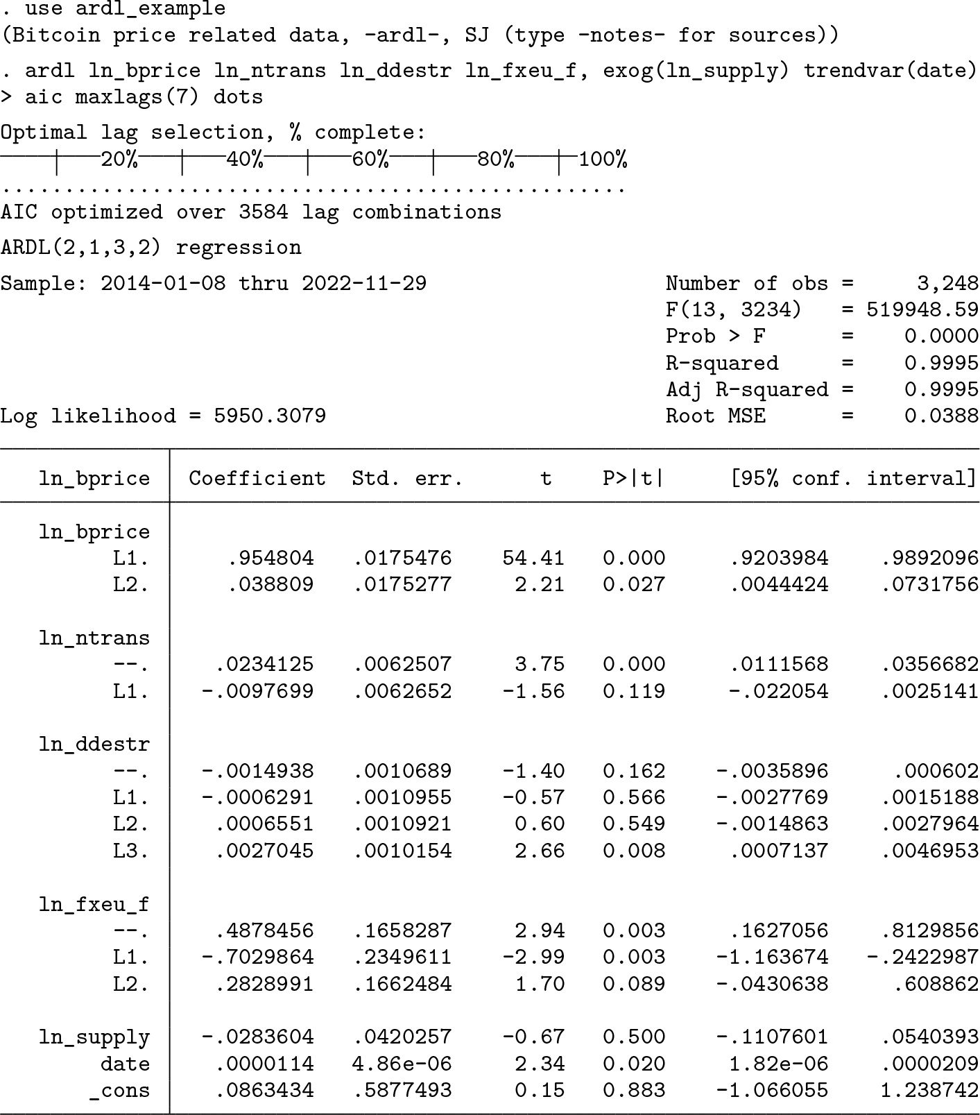We therefore add the maxlags(7) and aic options to our ardl command line. The quasideterministic supply variable is specified with the exog() option, which also constrains its lag order to zero. If we were to add it as a conventional independent variable instead, the command would error out because of collinearity of the lags.²⁷ To complete our specification, we add a linear time trend by including the name of the time identifier in the trend() option. While the optimization over all 3,584 lag combinations finishes in virtually no time using our fast Mata algorithm, we illustrate how to display a progress bar with the option dots, which might be useful for larger models:

The optimal model chosen by the AIC is an ARDL(2,1,3,2) model.²⁸ The supply of Bitcoin has no statistically significant effect, which could justify removing this regressor at a later stage. In contrast, the linear time trend, represented by the variable date, is statistically significant at the 5% level, in line with our earlier observations.²⁹ Before turning our attention to the bounds test, we should inspect the residuals for potential serial correlation:

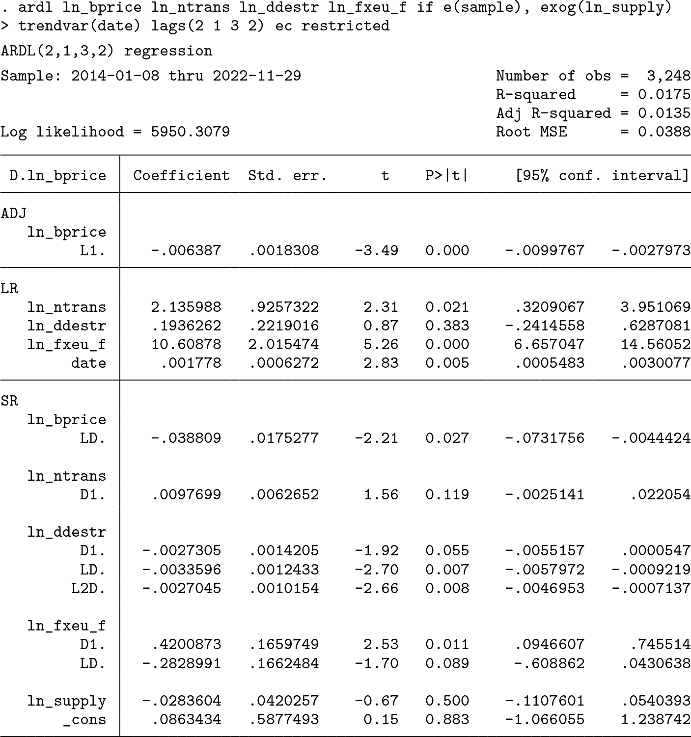
The Lagrange multiplier test does not provide reason for concern about residual serial correlation. We now refit the model in error-correction form—(6)—using the ec option. While the AIC would give us the same lag orders again, we can also directly specify the optimal lag orders with the lags() option. However, we then need to exert some caution to obtain results for the same estimation sample as above. Allowing for a maximum of seven lags, we set aside the first seven data points for the optimal lag determination. The estimation sample was held fixed by the ardl command even for models with lower lag orders. To base the bounds test again on the same estimation sample, we restrict it in the next step with the e(sample) function. To obtain the correct CVs with the bounds test for case 4, we now also need to add the option restricted, which includes the time trend in the long-run relationship:

The first coefficient in the ADJ section of the regression output is the negative speedof-adjustment coefficient π_y = −α. Its magnitude is very small. At this stage, we should not be fooled by the reported p-value and confidence interval into believing that it is statistically significant. The t statistic for this coefficient does not have a standard distribution under the null hypothesis. In fact, this is the test statistic that we consider under the second step of the bounds test. The long-run coefficients θ in the LR section all have the expected sign. Coin days destroyed is statistically insignificant, which is not too surprising given the suspected differences in the integration orders. The trend coefficient (date) is reported in the LR section because of the option restricted. Without that option, it would be reported in the SR section together with the other short-run coefficients ω , ψ _xi , and γ . This does not affect any of the other coefficients, but it will matter for the bounds test. Because of first differencing, the lag orders for the short-run terms are one less than those in the ARDL level representation. Also, note that the exogenous supply variable is not transformed into first differences and just enters the model with the same coefficient as in the ARDL specification. Before we start interpreting the coefficient estimates, we first need to establish with the bounds test whether a longrun relationship exists. We do this with the estat ectest postestimation command:

In the top-right corner, the bounds-test output displays the test statistics for the first two testing steps, as outlined in section 2.3. The command reports the Kripfganz and Schneider (2020) CVs for finite samples. However, because of the large sample size, they are virtually identical with the asymptotic CVs.³⁰ First, we consider the F statistic for the joint null hypothesis π_y = 0, π _x = 0, and c ₁ = 0. The last coefficient captures the restriction on the time trend. The test statistic is larger than the upper-bound CVs—which would be the exact CVs if all long-run forcing variables were I(1)—for the conventional significance levels. This is most easily seen by looking at the approximate p-values, which are computed with the response-surface methodology of Kripfganz and Schneider (2020). We therefore reject the null hypothesis in this first step. However, this is not yet sufficient evidence in favor of a long-run relationship, because we need to rule out the degenerate cases.

Second, we need to consider the individual null hypothesis π_y = 0. The test statistic is the same as in the ADJ section of the regression output, but only estat ectest provides the appropriate CVs. Here the conclusion depends on the chosen significance level. If we take a conservative stance with the 1% level, the t statistic is closer to zero than the lower-bound CV. We would therefore not reject the null hypothesis. The statistical significance of the long-run coefficients in the EC regression output then becomes irrelevant, because the equilibrium correction term y_t ₋ ₁ − θx _t drops out from (6) with π_y = α = 0 under the null hypothesis. In the long run, the log Bitcoin price can thus be characterized by a unit-root process that is not driven by the independent variables in our model.

As we move to a more relaxed stance on the risk of committing a type-I error—rejecting the null hypothesis when it is actually true—the bounds test becomes inconclusive at the 5% significance level. Here the value of the t statistic falls inside the two bounds, although it exceeds the lower bound only narrowly. Given the presence of I(1) independent variables, the evidence still points more strongly toward not rejecting the null hypothesis. When we move further to the 10% level, the test statistic remains within the two bounds. Because the long-run coefficient of the only I(0) variable, coin days destroyed, is statistically insignificant, the upper-bound CV carries much more weight than the lower bound. As a way of resolving this inconclusiveness, we can redo the bounds test for a model without coin days destroyed:

Assuming that all integration orders are known to be I(1), the bounds test still fails to reject the null hypothesis because the t statistic is less negative than the upper-bound CV at all significance levels. At the 5% level, it now even falls short of the lower bound. Consequently, the statistical significance of the long-run coefficients is not informative. Evidence of a cointegrating relationship could not be established.³¹

We can cross-check results with the Johansen (1995) framework using the vecrank and vec commands. Here, unlike the ARDL framework, we should specify only nonstationary variables. To be on the safe side, we might want to initially run the augmented Dickey and Fuller (1979) unit-root pretest for each of the variables. This can be done with the dfuller command. Because this unit-root test is a special case of the bounds test when there is only one variable, we can also use our ardl command for this purpose. As an example, we show this for the Bitcoin price:³²

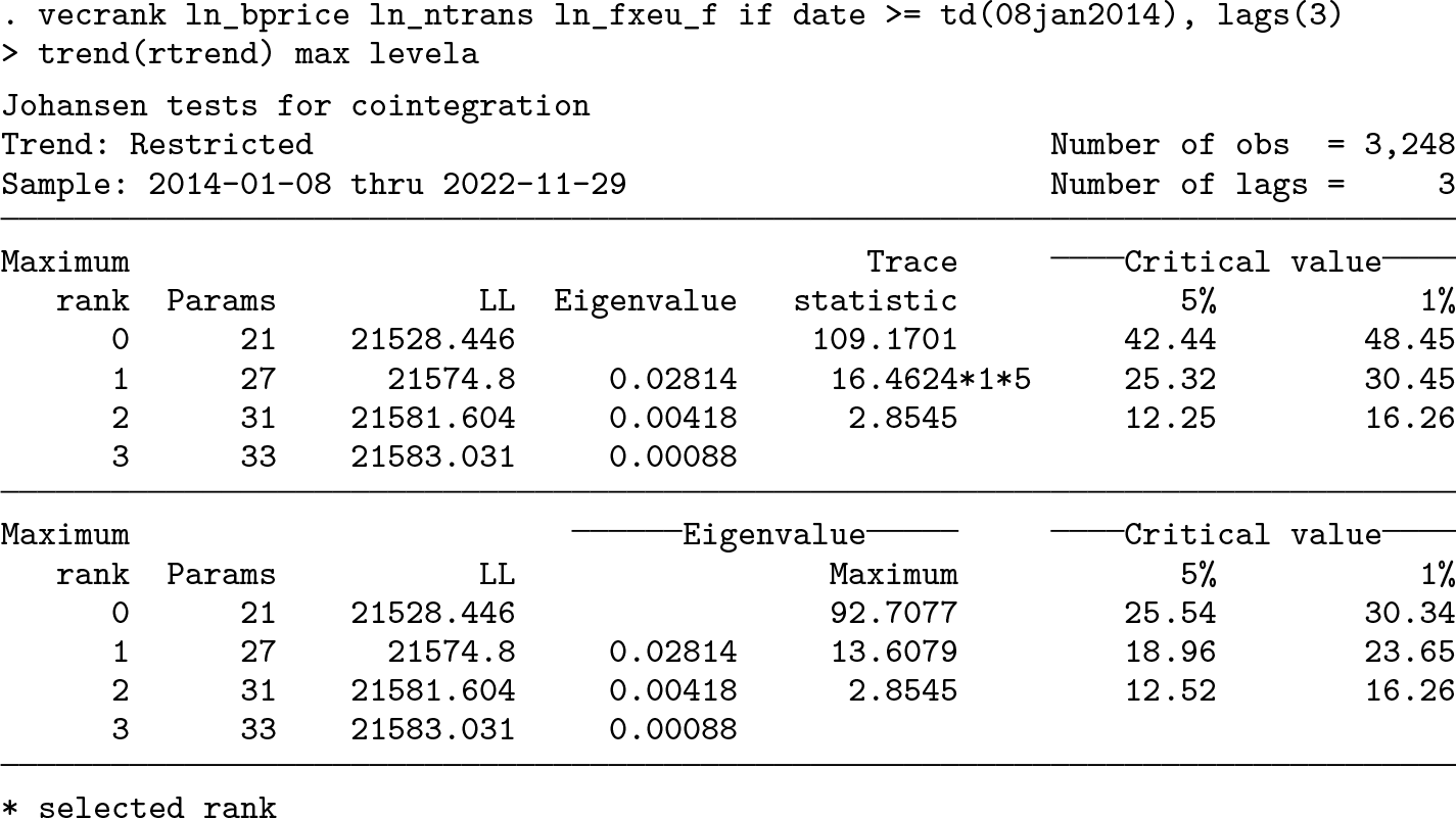
The t statistic from the bounds test equals the Dickey and Fuller (1979) test statistic. The CVs also virtually coincide.³³ The F test reported by estat ectest corresponds to the Dickey and Fuller (1981) F statistic, which is not implemented elsewhere in Stata. Both tests confirm our prior assessment that the log Bitcoin price is nonstationary. While not shown here, similar tests for the other variables also support our initial classification. We can now proceed with the cointegration rank tests. For the best comparability with the previous results, we choose a lag order of 3—which was the maximum lag order for any variable selected by the AIC in the ARDL model—and restrict the estimation sample again to coincide with the one above:

The Johansen (1995) trace and maximum-eigenvalue tests both indicate a cointegration rank of one. However, this is only a necessary but not sufficient condition for the presence of an error-correction mechanism in the process of the log Bitcoin price.³⁴ In the next step, we fit the VEC model:

Clearly, according to the bottom table for the speed-of-adjustment coefficients, the USD/EUR exchange rate is not loading onto the cointegrating relationship. The respective coefficient for the Bitcoin price is also very small. For practical matters, the Bitcoin price hardly reacts to deviations from the equilibrium relationship. Thus, the statistical question of whether there exists a long-run relationship should not bear too much weight in the final assessment, because it would take a very long time for the Bitcoin price to return to such an equilibrium. Somewhat problematic is the wrong sign of the statistically significant adjustment coefficient for the number of transactions. This points toward an instability in the system. By focusing only on the equation for the Bitcoin price, the ARDL approach avoids this issue. Another disadvantage of the vecrank command is that it does not allow inclusion of exogenous I(0) variables, unlike ardl. Furthermore, by estimating a system of equations, the number of coefficients to be estimated can be substantially larger in the VEC model. Notably, the long-run coefficients are broadly consistent with the ARDL results, even though their relevance should not be overstated because of the minuscule or nonexistent error adjustment.

So far, there is no convincing evidence in favor of a long-run relationship of the Bitcoin price with traditional supply and demand side characteristics. However, the demand for Bitcoin may generally depend on other or additional factors than those for well-established currencies and investment assets. For example, it may depend on how well the cryptocurrency market is understood and trusted by potential investors. Furthermore, macrofinancial developments can affect the willingness to invest in highrisk assets. Ciaian, Rajcaniova, and Kancs (2016) therefore include the number of views of Bitcoin’s Wikipedia page (wikivw) as a measure of investment attractiveness, the Dow Jones Industrial Average stock market index (djon_f) as a proxy for investor sentiment, and the Brent crude oil price (oprc_f) as an indicator of macroeconomic risks.³⁵ Given its statistical insignificance, we remove the Bitcoin supply in the following specifications.

To economize on space, we summarize the results for the speed-of-adjustment coefficient (ADJ) and the long-run coefficients (LR, excluding the linear time trend) in table 1 instead of showing detailed Stata output. For ease of comparability, column 1 repeats the results from our initial regression further above. Let us first look at column 2. The stock market index and the oil price index do not appear to be relevant long-run forcing variables for the Bitcoin price, irrespective of whether any long-run relationship exists in the first place. In contrast, the long-run coefficient of Wikipedia views is statistically significant. With its inclusion, the bounds test now also conclusively rejects the null hypothesis, although only at the 10% level. However, the economic significance of this result remains limited because of the very slow speed of adjustment. Compared with the benchmark specification in column 1, the main statistical reason for the reduction in the bounds-test p-values is the near doubling of the speed-of-adjustment coefficient, which is immediately reflected in a larger t statistic. However, this cannot mask the fact that the economic effect size is still negligible.

Table 1.

ARDL long-run estimation results in EC representation

					Column
	D.ln_bprice	1	2		3	4	5
date						>10jul2016	>10jul2016<12may2020
ADJ	L.ln_bprice	−0.006		−0.011	−0.011	−0.010	−0.011
LR	ln_ntrans	2.136^∗∗		1.285^∗∗∗	1.256^∗∗∗	1.556^∗∗	1.504^∗
	ln_ddestr	0.194		0.027	0.025	0.005	0.190
	ln_fxeu_f	10.609^∗∗∗		7.862^∗∗∗	7.838^∗∗∗	8.538^∗∗∗	9.054^∗∗
	ln_wikivw			0.315^∗∗∗	0.320^∗∗∗	0.422^∗∗	0.389^∗
	ln_djon_f			1.396	1.514	0.453	0.431
	ln_oprc_f			0.065	.	.
F		${6.156}_{* * }^{ * *}$		${5.198}_{* * }^{ * *}$	${5.934}_{* * }^{ * *}$	${3.985}_{* * }^{ *}$	${2.872}_{* *}$
t		$- {3.489}_{* *}$		$- {4.521}_{* * }^{}$	$- {4.522}_{* }^{}$	−3.355^∗	−2.706

NOTE: Stars indicate the significance level (^∗ p < 0.1; ^∗∗ p < 0.05; ^∗∗∗ p < 0.01.) Conventional p-values for the ADJ coefficient are invalid and thus not reported. For the bounds test, both upper-bound and lower-bound significance levels are indicated. A conclusive decision requires either significance or insignificance with respect to both the upper and lower bounds. Significance only with respect to the lower bound indicates inconclusiveness.

In column 3, we exclude the irrelevant oil prices from the model. Despite their insignificant long-run coefficients, we keep the stock market index and coin days destroyed because they still have significant short-run effects. The estimates hardly differ from the previous specification.

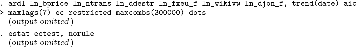
Over time, Bitcoin (and cryptocurrencies in general) became more and more accessible to a wider audience and also attracted the interest of professional investors. This may have lead to a gradual change in the fundamental relationship between the Bitcoin price and its determinants. In econometric terms, we may have to worry about parameter instability. 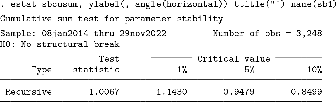Stata offers several diagnostics for structural breaks, which we can use here because the ardl command supports all standard postestimation commands for regress. A routinely applied tool is the cumulative sum (CUSUM) test:

Figure 2.

CUSUM plots

The CUSUM test based on OLS residuals does not trigger a warning sign. In contrast, the test based on recursive residuals rejects the null hypothesis of parameter stability at the 5% significance level. However, because the recursive CUSUM process travels beyond the 95% confidence bounds only very briefly, we may not have to worry too much. Figure 2 shows that the drift away from zero occurs rather gradually over time. This does not suggest a specific date for a structural break, other than that it may have occurred relatively early during our sample period. However, potential break points can be spotted in figure 1. While the Bitcoin supply did not turn out to be a relevant predictor in the earlier regressions, the discrete slowdowns in the mining of new Bitcoin at July 10, 2016, and May 12, 2020—so-called “halving dates”³⁶—could possibly have wider repercussions.

Indeed, a parameter stability test with these known structural-break dates rejects the null hypothesis. However, if we restrict the test to the speed-of-adjustment and long-run coefficients, no instability is found. The latter is reassuring regarding our earlier results. Accounting for structural breaks in the short-run coefficients would become a potential issue if we were interested in a more detailed analysis of the short-run dynamics. Nevertheless, as a robustness check, we refit the model by considering only the observations after the first halving date. In another specification, we further curtail the sample with the second halving date.

The main results are shown in columns 4 and 5 of table 1. The effect sizes hardly changed, especially for the speed of adjustment, which is instrumental for existence of an equilibrium correction mechanism. Interestingly though, the bounds test now does conclusively not reject the null hypothesis of no level relationship at least at the 5% significance level. Compared with the specifications in columns 2 and 3, this is mainly driven by the larger standard error of the speed-of-adjustment coefficient, partly because of the smaller sample size. Turning the argument around, the large size of the unrestricted sample—daily observations for almost nine years—previously enabled us to statistically detect (at the 10% significance level) an economically insignificant effect.

As a word of caution, the reliability of the bounds test could be hampered by the nonnormality of the regression errors. Heteroskedasticity and normality tests with the postestimation commands estat hettest and estat imtest tend to point in that direction (not shown here).³⁷ This is not unexpected when working with financial data. Ideas for further exploration include the incorporation of potential asymmetric effects and other nonlinearities, a quest for alternative explanatory variables, or a generalized autoregressive conditional heteroskedasticity modeling approach. We leave these avenues to the interested reader.

Overall, based on the results presented here, there do not seem to be strong forces in place that keep the log Bitcoin price in an equilibrium relationship with the candidate long-run forcing variables. Even if we accept column 2 or 3 as our preferred specification and take a liberal stand on the type-I error probability, the economic relevance of the rejected bounds test remains negligible because of the slow speed of adjustment. It appears that the price of Bitcoin is hardly driven by the underlying fundamentals but might be following the path of a predominantly speculative asset. If we accept the statistical conclusion from one of the other specifications that there is no significant long-run relationship present, we could proceed by refitting a more parsimonious version of the model purely in first differences, potentially also using the BIC instead of the AIC as a lag order selection criterion. This could then be used for forecasting purposes or further analyses of the dynamic adjustment processes. For the purpose of this article, however, our curiosity shall end here.³⁸

6 Conclusion

In this article, we have described the ardl command for the estimation of ARDL models with time-series data. The lag orders can be prespecified or chosen optimally with the AIC or BIC. For this purpose, the command is able to fit tens of thousands of candidate models in virtually no time. Two useful reparameterizations of the model in error-correction form allow for an interpretation of the coefficients as short-run and long-run effects. The command further enables testing for the existence of a long-run level relationship using the popular bounds test, which is implemented as a postestimation feature. For nonstationary variables, this amounts to cointegration testing. Yet the ARDL approach is flexible to allow for both stationary and nonstationary variables. The package provides the recently improved Kripfganz and Schneider (2020) CVs for the bounds test, which allow accurate inference for almost all practically relevant combinations of sample size, number of long-run forcing variables, lag orders, and deterministic model components.

8 Programs and supplemental material

Supplemental Material, sj-zip-1-stj-10.1177_1536867X231212434 - ardl: Estimating autoregressive distributed lag and equilibrium correction models

Supplemental Material, sj-zip-1-stj-10.1177_1536867X231212434 for ardl: Estimating autoregressive distributed lag and equilibrium correction models by Sebastian Kripfganz and Daniel C. Schneider in The Stata Journal

Footnotes

7 Acknowledgments

We thank Michael Binder for his support and guidance during early stages of this project. Moreover, we are grateful for numerous comments and suggestions from the Stata community that helped to improve our ardl package. This includes countless email communications, discussions on the Statalist forum, and exchanges of ideas at the 2016 Stata Conference in Chicago, the 2017 and 2018 German Stata Users Group meetings in Berlin and Konstanz, respectively, and the 2018 U.K. Stata Conference in London.

8 Programs and supplemental material

To install the software files as they exist at the time of publication of this article, type

Notes

References

Adeleye

Osabuohien

Bowale

Matthew

Oduntan

. 2018. Financial reforms and credit growth in Nigeria: Empirical insights from ARDL and ECM techniques. International Review of Applied Economics 32: 807–820. https://doi.org/10.1080/02692171.2017.1375466.

Ang

J. B.

2007. CO₂ emissions, energy consumption, and output in France. Energy Policy 35: 4772–4778. https://doi.org/10.1016/j.enpol.2007.03.032.

Ang

J. B.

2010. Finance and inequality: The case of India. Southern Economic Journal 76: 738–761. https://doi.org/10.4284/sej.2010.76.3.738.

Aruga

Islam

M. M.

Jannat

. 2020. Effects of COVID-19 on Indian energy consumption. Southern Economic Journal 12: 5616. https://doi.org/10.3390/su12145616.

Bahmani-Oskooee

Brooks

T. J.

. 1999. Bilateral J-curve between U.S. and her trading partners. Weltwirtschaftliches Archiv 135: 156–165. https://doi.org/10.1007/BF02708163.

Bekun

F. V.

Emir

Sarkodie

S. A.

. 2019. Another look at the relationship between energy consumption, carbon dioxide emissions, and economic growth in South Africa. Science of the Total Environment 655: 759–765. https://doi.org/10.1016/j.scitotenv.2018.11.271.

Belloumi

2014. The relationship between trade, FDI and economic growth in Tunisia: An application of the autoregressive distributed lag model. Economic Systems 38: 269–287. https://doi.org/10.1016/j.ecosys.2013.09.002.

Blackburne

E. F.

III Frank

M. W.

. 2007. Estimation of nonstationary heterogeneous panels. Stata Journal 7: 197–208. https://doi.org/10.1177/1536867X0700700204.

Büyükşahin

Robe

M. A.

. 2014. Speculators, commodities and cross-market linkages. Journal of International Money and Finance 42: 38–70. https://doi.org/10.1016/j.jimonfin.2013.08.004.

10.

Ciaian

Rajcaniova

Kancs

. 2016. The economics of BitCoin price formation. Applied Economics 48: 1799–1815. https://doi.org/10.1080/00036846.2015.1109038.

11.

Ciaian

Rajcaniova

Kancs

. 2018. Virtual relationships: Short- and long-run evidence from BitCoin and altcoin markets. Journal of International Financial Markets, Institutions and Money 52: 173–195. https://doi.org/10.1016/j.intfin.2017.11.001.

12.

Davis

E. P.

Zhu

. 2011. Bank lending and commercial property cycles: Some cross-country evidence. Journal of International Money and Finance 30: 1–21. https://doi.org/10.1016/j.jimonfin.2010.06.005.

13.

De Vita

Abbott

. 2004. Real exchange rate volatility and U.S. exports: An ARDL bounds testing approach. Economic Issues 9: 69–78.

14.

Dickey

D. A.

Fuller

W. A.

. 1979. Distribution of the estimators for autoregressive time series with a unit root. Journal of the American Statistical Association 74: 427–431. https://doi.org/10.2307/2286348.

15.

Dickey

D. A.

Fuller

W. A.

. 1981. Likelihood ratio statistics for autoregressive time series with a unit root. Econometrica 49: 1057–1072. https://doi.org/10.2307/1912517.

16.

Ditzen

2018. Estimating dynamic common-correlated effects in Stata. Stata Journal 18: 585–617. https://doi.org/10.1177/1536867X1801800306.

17.

Dickey

D. A.

Fuller

W. A.

. 2021. Estimating long-run effects and the exponent of cross-sectional dependence: An update to xtdcce2. Stata Journal 21: 687–707. https://doi.org/10.1177/1536867X211045560.

18.

Doğan

Jebli

M. B.

Shahzad

Farooq

T. H.

Shahzad

. 2020. Investigating the effects of meteorological parameters on COVID-19: Case study of New Jersey, United States. Environmental Research 191: 110148. https://doi.org/10.1016/j.envres.2020.110148.

19.

Engle

R. F.

Granger

C. W. J.

. 1987. Co-integration and error correction: Representation, estimation, and testing. Econometrica 55: 251–276. https://doi.org/10.2307/1913236.

20.

Enisan

A. A.

Olufisayo

A. O.

. 2009. Stock market development and economic growth: Evidence from seven sub-Sahara African countries. Journal of Economics and Business 61: 162–171. https://doi.org/10.1016/j.jeconbus.2008.05.001.

21.

Esaku

2022. Institutionalized democracy and the shadow economy in the short- and long-run: Empirical analysis from Uganda. Humanities and Social Sciences Communications 9: 165. https://doi.org/10.1057/s41599-022-01128-1.

22.

Fatai

Oxley

Scrimgeour

F. G.

. 2004. Modelling the causal relationship between energy consumption and GDP in New Zealand, Australia, India, Indonesia, The Philippines and Thailand. Mathematics and Computers in Simulation 64: 431–445. https://doi.org/10.1016/S0378-4754(03)00109-5.

23.

Fedderke

J. W.

Perkins

Luiz

J. M.

. 2006. Infrastructural investment in longrun economic growth: South Africa 1875–2001. World Development 34: 1037–1059. https://doi.org/10.1016/j.worlddev.2005.11.004.

24.

Frankel

Schmukler

S. L.

Servén

. 2004. Global transmission of interest rates: Monetary independence and currency regime. Journal of International Money and Finance 23: 701–733. https://doi.org/10.1016/j.jimonfin.2004.03.006.

25.

Halicioglu

2009. An econometric study of CO₂ emissions, energy consumption, income and foreign trade in Turkey. Energy Policy 37: 1156–1164. https://doi.org/10.1016/j.enpol.2008.11.012.

26.

Hassler

Wolters

. 2006. Autoregressive distributed lag models and cointegration. Allgemeines Statistisches Archiv 90: 59–74. https://doi.org/10.1007/s10182-006-0221-5.

27.

Zhang

Cai

Aoyagi

. 2017. Construction and evaluation of two computational models for predicting the incidence of influenza in Nagasaki Prefecture, Japan. Scientific Reports 7: 7192. https://doi.org/10.1038/s41598-017-07475-3.

28.

Jalil

Mahmud

S. F.

. 2009. Environment Kuznets curve for CO₂ emissions: A cointegration analysis for China. Energy Policy 37: 5167–5172. https://doi.org/10.1016/j.enpol.2009.07.044.

29.

Johansen

. 1995. Likelihood-Based Inference in Cointegrated Vector Autoregressive Models. Oxford: Oxford University Press. https://doi.org/10.1093/0198774508.001.0001.

30.

Jordan

Philips

A. Q.

. 2018. Cointegration testing and dynamic simulations of autoregressive distributed lag models. Stata Journal 18: 902–923. https://doi.org/10.1177/1536867X1801800409.

31.

Katircioglu

S. T.

2009. Revisiting the tourism-led-growth hypothesis for Turkey using the bounds test and Johansen approach for cointegration. Tourism Management 30: 17–20. https://doi.org/10.1016/j.tourman.2008.04.004.

32.

Kirikkaleli

Güngör

Adebayo

T. S.

. 2022. Consumption-based carbon emissions, renewable energy consumption, financial development and economic growth in Chile. Business Strategy and the Environment 31: 1123–1137. https://doi.org/10.1002/bse.2945.

33.

Kripfganz

Sarafidis

. 2021. Instrumental-variable estimation of large-T panel-data models with common factors. Stata Journal 21: 659–686. https://doi.org/10.1177/1536867X211045558.

34.

Kripfganz

Schneider

D. C.

. 2020. Response surface regressions for critical value bounds and approximate p-values in equilibrium correction models. Oxford Bulletin of Economics and Statistics 82: 1456–1481. https://doi.org/10.1111/obes.12377.

35.

Kripfganz

Schneider

D. C.

. 2022. ardl: Estimating autoregressive distributed lag and equilibrium correction models. Research Center for Policy Design Discussion Paper 2TUPD-2022-006, Tohoku University. http://hdl.handle.net/10097/00135205.

36.

Lee

G. H. Y.

Lee

S. P.

. 2014. Childcare availability, fertility and female labor force participation in Japan. Journal of the Japanese and International Economies 32: 71–85. https://doi.org/10.1016/j.jjie.2014.01.002.

37.

Morley

2006. Causality between economic growth and immigration: An ARDL bounds testing approach. Economics Letters 90: 72–76. https://doi.org/10.1016/j.econlet.2005.07.008.

38.

Murthy

V. N. R.

Okunade

A. A.

. 2016. Determinants of U.S. health expenditure: Evidence from autoregressive distributed lag (ARDL) approach to cointegration. Economic Modelling 59: 67–73. https://doi.org/10.1016/j.econmod.2016.07.001.

39.

Narayan

P. K.

2005. The saving and investment nexus for China: Evidence from cointegration tests. Applied Economics 37: 1979–1990. https://doi.org/10.1080/00036840500278103.

40.

Narayan

P. K.

Smyth

. 2005. Electricity consumption, employment and real income in Australia evidence from multivariate Granger causality tests. Energy Policy 33: 1109–1116. https://doi.org/10.1016/j.enpol.2003.11.010.

41.

Narayan

P. K.

Smyth

Nandha

. 2004. Interdependence and dynamic linkages between the emerging stock markets of South Asia. Accounting and Finance 44: 419–439. https://doi.org/10.1111/j.1467-629x.2004.00113.x.

42.

Ntanos

Skordoulis

Kyriakopoulos

Arabatzis

Chalikias

Galatsidas

Batzios

Katsarou

. 2018. Renewable energy and economic growth: Evidence from European countries. Sustainability 10: 2626. https://doi.org/10.3390/su10082626.

43.

Obstfeld

Shambaugh

J. C.

Taylor

A. M.

. 2005. The trilemma in history: Tradeoffs among exchange rates, monetary policies, and capital mobility. Review of Economics and Statistics 87: 423–438. https://doi.org/10.1162/0034653054638300.

44.

Oteng-Abayie

E. F.

Frimpong

J. M.

. 2006. Bounds testing approach to cointegration: An examination of foreign direct investment trade and growth relationships. American Journal of Applied Sciences 3: 2079–2085.

45.

Persyn

Westerlund

. 2008. Error-correction–based cointegration tests for panel data. Stata Journal 8: 232–241. https://doi.org/10.1177/1536867X0800800205.

46.

Pesaran

M. H.

Shin

. 1998. An autoregressive distributed-lag modelling approach to cointegration analysis. In Econometrics and Economic Theory in the Twentieth Century: The Ragner Frisch Centennial Symposium, ed. Steiner

, 371–413. Cambridge: Cambridge University Press. https://doi.org/10.1017/CCOL521633230.011.

47.

Pesaran

M. H.

Shin

Smith

R. J.

. 2001. Bounds testing approaches to the analysis of level relationships. Journal of Applied Econometrics 16: 289–326. https://doi.org/10.1002/jae.616.

48.

Phillips

P. C. B.

Hansen

B. E.

. 1990. Statistical inference in instrumental variables regression with I(1) processes. Review of Economic Studies 57: 99–125. https://doi.org/10.2307/2297545.

49.

Sari

Hammoudeh

Soytas

. 2010. Dynamics of oil price, precious metal prices, and exchange rate. Energy Economics 32: 351–362. https://doi.org/10.1016/j.eneco.2009.08.010.

50.

Schaffer

M. E

. 2010. egranger: Stata module to perform Engle–Granger cointegration tests and 2-step ECM estimation. Statistical Software Components S457210, Department of Economics, Boston College. https://ideas.repec.org/c/boc/bocode/s457210.html.

51.

Shambaugh

J. C.

2004. The effect of fixed exchange rates on monetary policy. Quarterly Journal of Economics 119: 301–352. https://doi.org/10.1162/003355304772839605.

52.

Shin

Greenwood-Nimmo

. 2014. Modelling asymmetric cointegration and dynamic multipliers in a nonlinear ARDL framework. In Festschrift in Honor of Peter Schmidt: Econometric Methods and Applications, ed. Horrace

W. C.

Sickles

R. C.

, 281–314. New York: Springer. https://doi.org/10.1007/978-1-4899-8008-3_9.

53.

Song

Lin

Witt

S. F.

Zhang

. 2011. Impact of financial/economic crisis on demand for hotel rooms in Hong Kong. Tourism Management 32: 172–186. https://doi.org/10.1016/j.tourman.2010.05.006.

54.

Stoian

Iorgulescu

. 2020. Fiscal policy and stock market efficiency: An ARDL bounds testing approach. Economic Modelling 90: 406–416. https://doi.org/10.1016/j.econmod.2019.12.023.

55.

Vardi

Muchnik

Conway

Breakstone

. 2021. WikiShark: An online tool for analyzing Wikipedia traffic and trends. In WWW ‘21: Companion Proceedings of the Web Conference 2021, 558–571. New York: Association for Computing Machinery. https://doi.org/10.1145/3442442.3452341.

56.

Varona

Gonzales

J. R.

. 2021. Dynamics of the impact of COVID-19 on the economic activity of Peru. PLOS ONE 16: e0244920. https://doi.org/10.1371/journal.pone.0244920.

57.

Wang

2012. Long-run covariance and its applications in cointegration regression. Stata Journal 12: 515–542. https://doi.org/10.1177/1536867X1201200312.

58.

Wang

Y.-S.

2009. The impact of crisis events and macroeconomic activity on Taiwan’s international inbound tourism demand. Tourism Management 30: 75–82. https://doi.org/10.1016/j.tourman.2008.04.010.

59.

Wolde-Rufael

2006. Electricity consumption and economic growth: A time series experience for 17 African countries. Energy Policy 34: 1106–1114. https://doi.org/10.1016/j.enpol.2004.10.008.

60.

Zhang

Song

Wen

Liu

. 2021. Forecasting tourism recovery amid COVID-19. Annals of Tourism Research 87: 103149. https://doi.org/10.1016/j.annals.2021.103149.

61.

Zhang

Davidson

E. A.

Mauzerall

D. L.

Searchinger

T. D.

Dumas

Shen

. 2015. Managing nitrogen for sustainable development. Nature 528: 51–59. https://doi.org/10.1038/nature15743.