A command to estimate and interpret models of dynamic compositional dependent variables: New features for dynsimpie

Abstract

Philips, Rutherford, and Whitten (2016, Stata Journal 16: 662–677) introduced dynsimpie, a command to examine dynamic compositional dependent variables. In this article, we present an update to dynsimpie and three new adofiles: cfbplot, effectsplot, and dynsimpiecoef. These updates greatly enhance the range of models that can be estimated and the ways in which model results can now be presented. The command dynsimpie has been updated so that users can obtain both prediction plots and change-from-baseline plots using postestimation commands. With the new command dynsimpiecoef, various types of coefficient plots can also be obtained. We illustrate these improvements using monthly data on support for political parties in the United Kingdom.

1 Introduction

Compositional variables, which represent data with the property of a constant sum, are common to a wide range of empirical fields. Most commonly, these variables are made up of values that sum to 100% for each unit of analysis. Examples include party shares of the popular vote, budgetary expenditures across spending categories, and the percentages by weight of minerals in rocks. The properties of compositional variables are such that they require special treatment when they are modeled as dependent variables (Aitchison 1982). But, despite the prevalence of compositional variables, few software tools are available for modeling them, especially in cases where the data are measured for the same unit across multiple points in time.

Philips, Rutherford, and Whitten (2016a) introduced dynsimpie, a command to help estimate and interpret results from models of dynamic compositional dependent variables that we can write as y_tj , measured across categories j = 1, 2,…, J and over time points t = 1, 2,…, T . Following the notation used by Philips, Souza, and Whitten (2019), this command first transforms the dependent variable into J − 1 logged compositions

$s_{tj}=\mathrm{In}\left(\frac{y_{tj}}{y_{t1}}\right)\forall j\ne 1$

where the choice of the baseline category, j = 1, is irrelevant to subsequent inferences as long as it never takes on a value of 0. As discussed in Philips, Souza, and Whitten (2019), J − 1 error-correction model (ECM) equations are then estimated with the following specification,

${\text{Δs}}_{\text{tj}}{\text{= β}}_{\text{0j}}{\text{- α}}_{\text{j}}{\text{s}}_{\text{t-1,j}}{\text{+ βLjx}}_{\text{t-1}}{\text{+ βSjΔx}}_{\text{t}}{\text{+ ε}}_{\text{jt}}$

1

where

Δs_tj is the change in the logged ratio of dependent variable category “j” for j > 1 to baseline category j = 1 from time “t − 1” to time “t”,

β _0j are the constant terms,

x_t is a vector of independent variable values at time “t”,

−α_j are the adjustment parameters that measure the long-run error-correction processes,

βSj is a vector of short-run effects parameters,

βLj is a vector of parameters that can be combined with −α_j to calculate estimated long-run effects of changes in each independent variable, and

ε_jt is a stochastic disturbance term that may be correlated across the “j” equations.

Because of the extensive number of parameters estimated and the nonlinear nature of the resulting inferences, the original dynsimpie command also produced a graph to help with model interpretation. This graph, called a “change-from-baseline” plot, shows the results from a user-specified scenario in which there is a one-time change (shock) to the value of a chosen independent variable.

In this article, we present an update to dynsimpie. The updated dynsimpie suite of commands now comprises four ado-files: dynsimpie, cfbplot, effectsplot, and dynsimpiecoef. This suite of commands requires the installation of the clarify package (Tomz, Wittenberg, and King 2003) and coefplot package (Jann 2014). The base command, dynsimpie, has been substantially enhanced. ¹ Users may now specify multiple shock variables within a single option. They can similarly specify multiple shock values within only one option. With the updated command, users may choose between an ECM specification such as that in (1) and a lagged dependent variable (LDV) model specification such as

${\text{s}}_{\text{tj}}{\text{= φ}}_{\text{j}}{\text{s}}_{\text{t-1,j}}{\text{+ β}}_{\text{0j}}{\text{+ βsjx}}_{\text{t}}{\text{+ ε}}_{\text{jt}}$

2

where

φ_j is the parameter on the LDV that, together with the values of βsj, may be used to calculate long-run changes; and

all other terms are as defined above in (1).

Where users find that an LDV model is not appropriate, the new ecm option allows for an ECM. Additionally, users can estimate models with an interaction between explanatory variables of interest by specifying the interaction( string ) and intype() options.

With the postestimation commands—cfbplot and effectsplot—users can now easily obtain change-from-baseline plots and prediction plots. These postestimation commands produce plots displaying the model-based simulations of both the shortand long-run effects on each category of the compositional dependent variable. Short for “change-from-baseline” plot, cfbplot displays a plot of the simulated output. The expected proportion of each of the compositional dependent variables is plotted across time, along with the associated confidence intervals. This was the only plot type available with the original version of dynsimpie. In this updated dynsimpie package, the postestimation command effectsplot displays effects plots (prediction plots) from estimated dynsimpie results.

The new command dynsimpiecoef produces various plots of the seemingly unrelated regression (SUR) coefficient results used in dynsimpie. In doing this, dynsimpiecoef allows two different ways of presenting the same information: displaying coefficients organized by dependent variable category or by independent variable. We illustrate these improvements using compositional data on monthly voter support for the political parties in the United Kingdom.

2 The dynsimpie command

2.1 Syntax

The syntax of the dynsimpie command is as follows:

dynsimpie indepvars [if] [in] , dvs( varlist ) [ecm ar( numlist )

shockvars( varlist ) shockvals( numlist ) dummy( varlist ) dummyset( numlist ) dummyshockvar( varname ) interaction( varname ) intype( string ) time( # )

sigs( numlist ) range( # ) percentage pv killtable]

indepvars is a list of continuous independent variables to be included in the model that do not experience a counterfactual shock. Notice that dynsimpie automatically transforms these variables (and any additional variables specified in other options) into lags and first differences for estimation in error-correction form when ecm is specified. By default, dynsimpie runs an LDV model. Other options allow for the addition of dummy variables to the model, provide the ability to shock multiple independent variables at the same point in time, and estimate multiplicative interactions.

2.2 Options

dvs( varlist ) is a list of the component parts of the compositional dependent variable. Each of these should be expressed either as proportions (summing to 1) or as percents (summing to 100). dynsimpie will issue an error message if neither of these criteria is met. dynsimpie will take the log of the proportion of each category relative to the proportion of an arbitrary “baseline” category. For instance, if there were J dependent variable categories in dvs(), dynsimpie would create J − 1 variables s_tj = ln(y_tj/y_{t 1}), where the first category, y_{t 1}, is the baseline. dvs() is required.

ecm specifies the choice of an ECM. It automatically transforms the dependent variables and independent variables into lags and first differences for estimation in errorcorrection form. The default is to estimate an LDV model.

ar( numlist ) is a numeric list of dependent variable lags to be included in the model. Up to three values may be inputted following Stata’s numlist conventions, and they need not be consecutive. This option is not allowed with ecm but is required in its absence.

shockvars( varlist ) is a list of continuous independent variables that are subject to counterfactual one-period shocks specified in shockvals(). The time in which all shocks enter the model is specified in time(). The variables listed in shockvars() must not be simultaneously included in indepvars. When an error-correction modeling technique is chosen by specifying ecm, the shock first affects the first-differenced values of the chosen variable at time t for one time period. This shock then affects the lag of the variable specified in shockvars(), starting at t + 1 and lasting through the rest of the simulated period. Failure to specify both this option and dummyshockvar() will lead to an all-baseline simulation. At most, users can specify three variables in shockvars().

shockvals( numlist ) is a numeric list of the amount to shock each respective variable in shockvars() for one period at time t, specified in time(). The number of values in shockvals() must be equal to the number of variables in shockvars().

dummy( varlist ) is a vector of dummy variables in the model. In dynsimpie, dummy variables enter the estimation equation in lagged form and first-differenced form if ecm is also specified. This is not the case in dynsimpiecoef, which takes dummy() exactly as specified.

dummyset( numlist ) specifies alternative values for each of the dummy variables specified in dummy() to be used throughout the simulation. By default, each of the dummy variables in dummy() will be set to 0 throughout the simulation.

dummyshockvar( varname ) is a dummy variable that is subject to a counterfactual oneperiod shock at time t, specified in time(). Variables specified in dummyshockvar() must not be simultaneously specified in dummy(). When ecm is specified, the shock first affects the first-differenced dummyshockvar() at time t for one time period. This shock then affects the lagged dummyshockvar(), starting at t + 1, and lasts through the rest of the period. Failure to specify both this option and shockvars() will lead to an all-baseline simulation.

interaction( varname ) is a dichotomous variable, not included as a control or shock variable elsewhere, to enter a multiplicative interaction. In dynsimpie, the variable entered in interaction() is interacted with the first variable listed in shockvars().

intype( string ) may be specified as intype(on) or intype(off). The variable specified in interaction() takes the value 1 when intype() is on and 0 when intype() is off. This option is not allowed with ecm.

time( # ) is the time in which the variables specified in the options shockvars() and dummyshockvar() experience a one-period shock. The default is time(5).

sigs( numlist ) is a numeric list of the significance levels for the percentile confidence intervals. The default is for 95% confidence intervals. At most, two significance levels may be listed in sigs().

range( # ) gives the length of the scenario to simulate. range( # ) must always be more than the time( # ) at which the shock occurs. The default is range(20).

percentage produces plots of percentages instead of plots of expected proportions, the default.

pv calculates predicted proportions instead of expected proportions, the default.

killtable suppresses the automatic generation of the SUR results. By default, a table of estimates is displayed in the Results window.

Note that users may also specify time lags or differences of independent variables in shockvars() and indepvars. Time lags (but not time differences) may also be specified for dummy variables in dummyshockvar(), dummy(), and interaction(). To specify lags or differences, users must use Stata’s time-series operators (for example, L1., L2., D., etc.). Manually generating and saving lagged or differenced variables and then entering them in the command will lead to incorrectly induced shocks, because the command will not be able to recognize the type of time-series transformation previously performed on the variable. In no instance should users use time-series operators when ecm is specified (because the command automatically performs the relevant time-series transformations in this case).

2.3 dynsimpie postestimation

The postestimation commands available after dynsimpie are the following: cfbplot and effectsplot. cfbplot displays a change-from-baseline plot of the simulated output. The expected proportion of each of the compositional dependent variables is plotted against time, along with the associated confidence intervals. effectsplot displays effects plots (prediction plots) from estimated results. This produces plots that visualize longand short-run effects of each of the compositional dependent variables, along with the associated confidence intervals. This is akin to a marginal effects plot.

3 The dynsimpiecoef command

3.1 Syntax

The syntax for dynsimpiecoef is

dynsimpiecoef indepvars [if] [in] , dvs( varlist ) [ecm ar( numlist )

dummy( varlist ) interaction( varname ) smooth sigs( numlist ) row( # )

xsize( # ) all vertical angle( angle ) killtable]

indepvars is a list of continuous independent variables to be included in the model that do not experience a counterfactual shock.

3.2 Options

dvs( varlist ) is a list of the component parts of the compositional dependent variable. Each of these should be expressed either as proportions (summing to 1) or as percents (summing to 100). dynsimpiecoef will take the log of the proportion of each category relative to the proportion of an arbitrary “baseline” category. dvs() is required.

ecm specifies the choice of an ECM. It automatically transforms the dependent variables and independent variables into lags and first differences for estimation in errorcorrection form. The default is to estimate an LDV model; it is not allowed with ar().

ar( numlist ) is a numeric list of dependent variable lags to be included in the model. Up to three values may be inputted following Stata’s numlist conventions, and they need not be consecutive. This option is not allowed with ecm but is required in its absence.

dummy( varlist ) is a vector of dummy variables in the model. In dynsimpie, dummy variables enter the estimation equation in lagged form and first-differenced form. This is not the case in dynsimpiecoef, which takes dummy() exactly as specified.

interaction( varname ) is a dichotomous variable, not included as a control or shock variable elsewhere, to enter a multiplicative interaction. In dynsimpiecoef, the variable entered in interaction() is interacted with the first variable listed in indepvars. interaction() is optional but, when specified, must be coded 0/1. This option is not allowed with ecm.

smooth adds confidence intervals for “50 equally spaced levels (1, 3,…, 99) with graduated color intensities and varying line widths”, as in coefplot (Jann 2014, 729). By default, dynsimpiecoef will generate coefficient plots with 95 percent confidence intervals. sigs() must not be specified with smooth.

sigs( numlist ) is a numeric list of the significance levels for the percentile confidence intervals. The default is for 95% confidence intervals. At most, two significance

levels may be listed in sigs().

row( # ) specifies the number of rows of the combined graph. Depending on the number of categories of the dependent variable and the number of independent variables in the model, a combined graph with multiple rows might be desirable. The default is row(1) if vertical is not specified. The default is row(3) with the vertical option.

xsize( # ) specifies the width of the combined graph in inches. Depending on the number of categories of the dependent variable and the number of independent variables in the model, it might be desirable to make the combined graph wider than usual using this option. The default is xsize(5).

all allows users to compare SUR results for all pairs of dependent variable categories. If specified, dynsimpiecoef automatically produces coefficient plots for all possible compositions of dependent variable categories, regardless of the baseline category. Thus, the order of dependent variable categories specified in dvs( varlist ) does not matter in dynsimpiecoef.

vertical specifies that dynsimpiecoef create coefficient plots for a particular independent variable across all possible pairwise compositions of dependent variable categories. With this option, dynsimpiecoef produces a collection of coefficient plots for each independent variable and saves coefficient plots for such variables automatically and separately in the working directory.

angle( angle ) specifies the angle for the labels on the x axis in the combined graph. This can only be specified with the vertical option. The default is angle(90), meaning that all labels are plotted at a 90-degree angle from the x axis.

killtable suppresses the automatic generation of the SUR results. By default, a table of estimates is displayed in the Results window.

4 Examples: dynsimpie

4.1 LDV models

By default, the dynsimpie command allows users to estimate effects of explanatory variables on compositional outcomes through an LDV model specification such as (2) that is estimated as a system of SURs. This command allows users to include lags of dependent and independent variables as well as a multiplicative interaction between a dichotomous independent variable of choice and a continuous shock variable. To illustrate the functionality of the new commands, we use the same monthly UK party support data as Philips, Rutherford, and Whitten (2016b,a). These data are from the 2004–2010 period when the Labour Party was in government and include the switch in Labour leader and thus prime minister from Tony Blair to Gordon Brown. During this period, the three main political parties were Labour, the Conservatives, and the Liberal Democrats. In our examples, support for these three main political parties are the categories of our dependent variable. ²

Imagine that we are interested in estimating the effect of a 1-standard-deviation increase in the average national economic retrospective evaluations on UK party support, while controlling for the percentage of respondents identifying with the party of the prime minister. Further imagine that we have theoretical reason to believe that the previous period’s composition of party support affects the current period. Finally, we expect the effect to differ between Gordon Brown’s and Tony Blair’s tenures.

The dynsimpie command can model these expectations well by including a multiplicative interaction and an LDV as shown in the code. Because intype() is on, the interaction variable is assumed to be 1 (Brown is in power). The option killtable is included to omit a regression table from the Results window in Stata. Notice that we use the cfbplot postestimation command to produce a change-from-baseline plot.

Figure 1.

Left panel: the simulated expected values of compositions over time with a 1-standard-deviation increase in the monthly average retrospective evaluation of the economy at t = 5. Right panel: the simulated effects from the same shock using the sigs(90 95) option in dynsimpie.

This plot is shown on the left panel in figure 1. An effects plot can be produced with a different postestimation command, effectsplot, shown on the right panel of figure 1. Notice that the shortand long-run effects depicted here are the same or very close to each other. ³ This is because they are essentially two different ways of displaying the effects from the same shock.

To evaluate interaction effects between any two variables, researchers often produce figures and estimates of the effects of one of these variables while holding the other variable at specific values. In our case, it makes sense to evaluate simulation results from shocks to a primary shock variable, listed first in shockvals(), at two distinct values of the dichotomous interaction variable. The intype() option helps with this. When intype() is set to on, as in figure 1, we observe the effect of a shock to shockvars(), while the interaction variable is held at 1 (Brown government, in our running example). In figure 2, we reproduce these figures with intype() set to off—where the interaction variable is held at 0 (Blair government). The code for the plots on the left and right panels of figure 2 is as follows:

Figure 2.

Left panel: the simulated expected values of compositions over time with a 1-standard-deviation increase in the monthly average retrospective evaluation of the economy at t = 5. Right panel: the simulated effects from the same shock using the sigs(90 95) option in dynsimpie.

Updating dynsimpie to allow for non-error-correction modeling contributes to a vastly more flexible command. Users can now use dynsimpie when an ECM is not warranted (such as when cointegration is not present). As a result, users can experiment with adding or removing time differences and lags among the independent variables as they see fit. Additionally, users can introduce a multiplicative interaction with one of the shock variables, which is useful in many theoretical contexts. Together, these additions to the command largely expand the domain of modeling choices available to users.

4.2 ECM

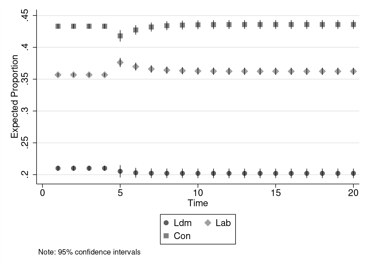
Users who find that an ECM is statistically and theoretically warranted can specify the option ecm to estimate an ECM-based dynsimpie. We again use the UK party support data to illustrate this. We list five control variables in indepvars and an additional shock variable in shockvars(): the percentage of those who view Labour as the best manager of the most important issue. Labour, Conservatives, and Liberal Democrats are the three dependent variable categories listed in the required dvs() option. In our dynamic simulations, we induce a 1-standard-deviation increase (+0.054) in the percentage of those who think Labour is the best manager of the most important issue at time t = 5.

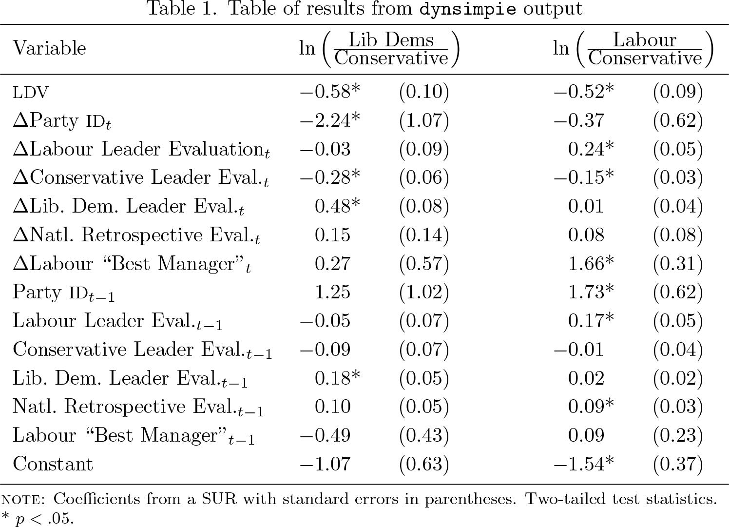
Given the three dependent variable categories, the dynsimpie command automatically performs log-ratio transformations and creates two log-ratio compositions: ln(Lib Dems/Conservative) and ln(Labour/Conservative). ⁴ The SUR results, produced by default when the option killtable is not specified, is shown in table 1. The coefficients in table 1 are plotted side by side across dependent variable categories.

Table 1.

Table of results from dynsimpie output

Variable	$\text{In}\left(\frac{\text{Lib Dems}}{\text{Conservative}}\right)$		$\text{In}\left(\frac{\text{Labour}}{\text{Conservative}}\right)$
LDV	−0.58*	(0.10)	−0.52*	(0.09)
ΔParty IDt	−2.24*	(1.07)	−0.37	(0.62)
ΔLabour Leader Evaluationt	−0.03	(0.09)	0.24*	(0.05)
ΔConservative Leader Eval.t	−0.28*	(0.06)	−0.15*	(0.03)
ΔLib. Dem. Leader Eval.t	0.48*	(0.08)	0.01	(0.04)
ΔNatl. Retrospective Eval.t	0.15	(0.14)	0.08	(0.08)
ΔLabour “Best Manager"	0.27	(0.57)	1.66*	(0.31)
Party IDt −1	1.25	(1.02)	1.73*	(0.62)
Labour Leader Eval.t −1	−0.05	(0.07)	0.17*	(0.05)
Conservative Leader Eval.t −1	−0.09	(0.07)	−0.01	(0.04)
Lib. Dem. Leader Eval.t −1	0.18*	(0.05)	0.02	(0.02)
Natl. Retrospective Eval.t −1	0.10	(0.05)	0.09*	(0.03)
Labour ‘‘Best Manager"t −1	−0.49	(0.43)	0.09	(0.23)
Constant	−1.07	(0.63)	−1.54*	(0.37)

NOTE: Coefficients from a SUR with standard errors in parentheses. Two-tailed test statistics. * p < .05.

We also present the predicted probabilities, shown in figure 3, generated using the cfbplot postestimation command. The figure shows both shortand long-run effects of the counterfactual shock on the expected proportion of party support in the UK across the simulated time period.

Figure 3.

The simulated effect of a 1-standard-deviation increase in the percentage of those who think Labour is the best manager of the most important issue

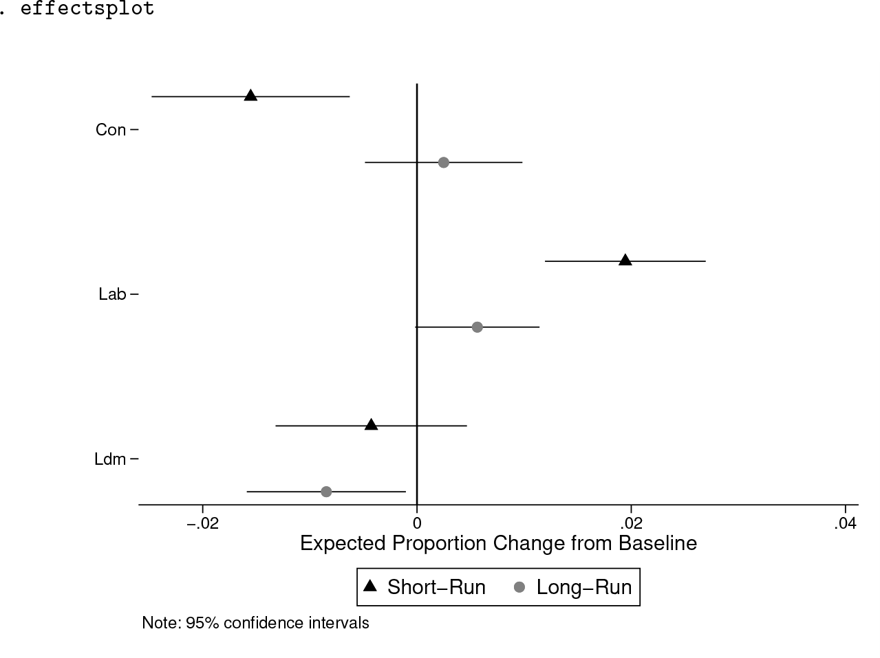
We now use another postestimation command, effectsplot, to create an effects plot (prediction plots) from the estimated dynsimpie results. This postestimation command allows users to easily produce plots that display the shortand long-run effects from the specified shock. The resulting effects plot is shown in figure 4 below.

Figure 4.

The simulated effect of a 1-standard-deviation increase in the percentage of those who think Labour is the best manager of the most important issue

As discussed above, the change-from-baseline and effects plots are two different ways of viewing the estimated effects of any shock. In either figure, it can be seen that Labour received a two-percentage point boost in the short run in response to the shock. This comes mainly at the expense of Conservative support. Nevertheless, over the long run, it is in fact the Liberal Democrats that experience a drop in support, whereas support for Conservatives returns to its starting value. Labour support diminishes and eventually settles just above its starting value. This long-run effect on support for Labour, however, turns out to be statistically insignificant at the 95% confidence level.

Additional confidence intervals can now be added to provide more information about the statistical and substantive significance of the simulation results. In the following example, we specify sigs(95 99) for both 95% and 99% confidence intervals. This is shown in figure 5.

Figure 5.

The simulated effect of a 1-standard-deviation increase in the percentage of those who think Labour is the best manager of the most important issue, created using the sigs(95 99) option

We will now briefly describe the other available options. For more detailed information, please refer to Philips, Rutherford, and Whitten (2016b,a). The time() option changes the time in the simulated scenario at which the independent variable receives a shock, while the range() option specifies the length of the scenario to simulate. Users can add one or more dummy variables to their model. For example, users may include a dummy variable that is equal to 1 during the months of the Great Recession using the dummy() option. By default, any dummy variables are set to zero in the simulations. Users can set this variable to 1 (or other values) using the option dummyset().

Users may include up to three continuous shocks to occur at the same point in time using the shockvars() and shockvals() options. Also, users may include a dummy shock variable that experiences some counterfactual one-period shock of 1 at time t using dummyshockvar(). Dummy shock variables are set to 0 before the shock occurs. When this is within an error-correction framework (that is, when ecm is specified), the shock first affects the first difference of dummyshockvar() at time t for one period, then will move into the lagged dummyshockvar() for the rest of the simulation.

Users wishing to analyze both fundamental and estimation uncertainty can do so by generating predicted values with the pv option. By default, clarify simulations produce expected values. These average out fundamental variability, keeping only estimation uncertainty. Users may also specify the option percentage to produce plot values in percentages, instead of proportions.

5 Example: dynsimpiecoef

We use dynsimpiecoef to create coefficient plots of the SUR results used in dynsimpie. dynsimpiecoef displays sets of coefficient plots for each log-compositional ratio as shown in the tabular plot presented in table 1. By default, dynsimpiecoef also produces a table of estimates. The killtable option suppresses the automatic generation of the SUR results, just as in dynsimpie. Keep in mind that the option ecm can be used to specify an ECM instead of the default LDV model. When ecm is omitted, users have to specify the option ar( numlist )—the consecutive or nonconsecutive lags of the dependent variable to be included among the explanatory variables. Furthermore, when users specify interaction( varname ), a multiplicative interaction is produced between this variable and the first variable listed among indepvars. Figure 6 below depicts an LDV(2) model with a multiplicative interaction between a recession dummy and the first variable listed in indepvars.

Figure 6.

Coefficient plots from the LDV dynsimpiecoef results with two lags of the dependent variable and a multiplicative interaction

In figure 7, similar graphs are produced but now by using the ecm and sigs( numlist ) options. Additionally, we use xsize( # ) to specify the width of the combined graph in inches. Depending on the number of categories of the dependent variable and the number of independent variables in the model, it might be desirable to make the combined graph wider than usual using this option. The default is xsize(5).

Figure 7.

Coefficient plots from the dynsimpiecoef results, created using the sigs(95 99) option

While the plots in figure 7 are generated using specific confidence intervals, users may wish to produce confidence intervals using a wide range of confidence levels. With the smooth option, users can add “50 equally spaced levels (1, 3,…, 99) with graduated color intensities and varying line widths” (Jann 2014, 729). This is shown in figure 8.

Figure 8.

Coefficient plots from the dynsimpiecoef results, created using the smooth option

With the all option, the dynsimpiecoef command will produce coefficient plots for all possible pairs of dependent variable categories, regardless of the baseline category. Thus, the order of dependent variable categories specified in dvs() does not matter in dynsimpiecoef. An example of the output when using this option is shown in figure 9.

Figure 9.

Coefficient plots from the dynsimpiecoef results, created using the sigs(95 99) and all options

While the coefficient plots of each model are useful for judging the significance of coefficients, the dynsimpiecoef command can also create coefficient plots for a particular independent variable across all possible pairwise compositions of dependent variable categories. Using the vertical option, users can easily compare the impact of each covariate in the model across dependent variable categories. While this option produces a collection of coefficient plots for each independent variable, users can find coefficient plots for such variables saved automatically and separately in the working directory. ⁵ Using the angle( angle ) option, users can specify the angle for the labels on the x axis in the combined graph. This option can only be specified with the vertical option. The default is angle(90), for 90 degrees from the x axis. This is shown in figure 10. Additionally, the row( # ) option allows users to specify the number of rows of the combined graph. Depending on the number of categories of the dependent variable and independent variables in the model, a combined graph with multiple rows might be desirable. By default, dynsimpiecoef displays the resulting graph in one row when the vertical option is not specified. When the vertical option is specified, dynsimpiecoef displays the resulting graph in three rows, as shown in figure 10.

Figure 10.

Coefficient plots from the dynsimpiecoef results, created using the vertical and angle(45) options

6 Conclusion

We have substantially enhanced the dynsimpie suite of commands for Stata. With it, users will be able to estimate and interpret a wide range of dynamic models of compositional dependent variables. In this update, we incorporate considerable flexibility in both model specification choices and graphical visualization of results.

Supplemental Material

Supplemental Material, st0448_1 - A command to estimate and interpret models of dynamic compositional dependent variables: New features for dynsimpie

Supplemental Material, st0448_1 for A command to estimate and interpret models of dynamic compositional dependent variables: New features for dynsimpie by Yoo Sun Jung, Flávio D. S. Souza, Andrew Q. Philips, Amanda Rutherford and Guy D. Whitten in The Stata Journal