Sage Journals: Discover world-class research

Abstract

We introduce a new command, summclust, that summarizes the cluster structure of the dataset for linear regression models with clustered disturbances. The key unit of observation for such a model is the cluster. We therefore propose cluster-level measures of leverage, partial leverage, and influence and show how to compute them quickly in most cases. The measures of leverage and partial leverage can be used as diagnostic tools to identify datasets and regression designs in which cluster–robust inference is likely to be challenging. The measures of influence can provide valuable information about how the results depend on the data in the various clusters. We also show how to calculate two jackknife variance matrix estimators efficiently as a by-product of our other computations. These estimators, which are already available in Stata, are generally more conservative than conventional variance matrix estimators. The summclust command computes all the quantities that we discuss.

Keywords

st0733 summclust clustered data cluster–robust variance estimator CRVE grouped data high-leverage clusters influential clusters jackknife partial leverage robust inference

1 Introduction

It is now standard in many fields of economics and other disciplines to use cluster– robust inference for the parameters of linear regression models. In the most common case, each of the N observations is assigned to one of G disjoint clusters, which might correspond to, for example, families, schools, villages, hospitals, firms, industries, years, cities, counties, or states. The assignment of observations to clusters is assumed to be known, and observations in different clusters are assumed to be independent, but any pattern of heteroskedasticity or dependence is allowed within each cluster. Under these assumptions, a cluster–robust variance matrix (CRVE) yields asymptotically valid t tests, Wald tests, and confidence intervals. However, even when N is very large, the resulting inferences may be unreliable when G is not large or the clusters are not sufficiently homogeneous.

The literature on cluster–robust inference has grown rapidly recently. Cameron and Miller’s (2015) article is a classic survey article. Conley, Gonçalves, and Hansen (2018) survey a broader class of methods for dependent data. MacKinnon, Nielsen, and Webb (2023a) offer a comprehensive guide to empirical practice. As it discusses, there are two situations in which cluster–robust t tests and Wald tests are at risk of overrejecting to an extreme extent, even when G is not small. The first is when one or a few clusters are much larger than the rest, and the second is when the only “treated” observations belong to just a few clusters; Djogbenou, MacKinnon, and Nielsen (2019) discuss the first case, and MacKinnon and Webb (2017a,b, 2018) discuss the second. In both of these cases, one cluster (or a few of them) has high leverage, in that omitting this cluster has the potential to change the ordinary least-squares (OLS) estimates substantially. When that actually happens, a cluster is said to be influential.

The concepts of leverage and influence are normally applied at the observation level (Belsley, Kuh, and Welsch 1980), but they are equally applicable at the cluster level. Just as high-leverage observations can make heteroskedasticity-robust inference unreliable (Chesher 1989), so, too, can high-leverage clusters make cluster–robust inference unreliable. Just as highly influential observations may lead us to suspect that there is something wrong with the model or the data, so, too, may highly influential clusters. Any situation in which a few clusters have high leverage or high influence should be worrying.

There are at least two different concepts of leverage. The usual one focuses on fitted values or, equivalently, residuals. A cluster is said to have high leverage if removing it has the potential to greatly change the fitted values for that cluster. The second concept is partial leverage (Cook and Weisberg 1980). A cluster is said to have high partial leverage for the jth coefficient if removing that cluster has the potential to greatly change the estimate of the jth coefficient. We discuss both concepts in section 2.1.

Whether a cluster has high leverage, has high partial leverage, or is influential can depend on the sample in rather complicated ways. We provide a new command, summclust, that implements computationally efficient ways to identify high-leverage and influential clusters and provides several statistics that collectively summarize the cluster structure of the dataset. These can be useful for detecting cases in which cluster–robust inference may not be reliable. Our leverage and influence calculations also allow us to compute two cluster jackknife variance matrix estimators, which we refer to as CV₃ and CV_3J, at little additional cost. These estimators are already available in Stata by using either the vce(jackknife) option or the jackknife prefix. Recent work (Hansen 2022; MacKinnon, Nielsen, and Webb 2023c) suggests that CV₃ and CV_3J generally perform better in finite samples than more widely used CRVEs; see section 7.

The remainder of the article is organized as follows. The next section begins with a brief review of cluster–robust inference for linear regression models. Then section 2.1 introduces our new measures of leverage, partial leverage, and influence at the cluster level. Section 2.2 shows how our results can be used to compute the CV₃ and CV_3J jackknife variance matrix estimators. Section 2.3 discusses what quantities are reported by summclust and should, at least in some cases, be reported by the investigator.

Section 3 provides a detailed description of the summclust command, which computes these variance estimators and diagnostic measures. The command uses the following syntax:

summclust varlist , cluster( varname ) [options]

summclust has many options and can even be used by itself to fit a linear regression model with clustered disturbances. The last few sections of the article illustrate the use of summclust and provide evidence on the value of the measures that it calculates. Section 4 presents an empirical illustration in which measures of leverage, partial leverage, and influence are highly informative. Section 4 discusses several special cases in which some or all of these measures can be determined analytically. Section 6 briefly discusses two-way clustering, where summclust can be valuable even though it is not explicitly designed to handle this case. Section 7 describes some simulation experiments that suggest that it may be desirable to report many of the quantities calculated by summclust, and section 8 concludes.

2 Clustering, leverage, influence, and the jackknife

We focus on the linear regression model

y_{g} = X_{g} β + u_{g}, g = 1, \dots, G

where the data have been divided into G disjoint clusters. The gth cluster has N_g observations, so the sample size is $N = \sum_{g = 1}^{G} N_{g}$ . In (1), X _g is an N_g × k matrix of regressors, β is a k-vector of coefficients, y _g is an N_g -vector of observations on the regressand, and u_g is an N_g -vector of disturbances (or error terms). Of course, the X _g may be stacked into an N × k matrix X , and likewise the y _g and u _g may be stacked into N-vectors y and u so that (1) can be rewritten as y = Xβ + u .

Dividing the sample into clusters becomes meaningful only if we make assumptions about the disturbance vectors u _g and, consequently, the score vectors $s_{g} = X_{g}^{⊤} u_{g}$ . For a correctly specified model, E( s _g ) = 0 for all g. We further assume that

E (s_{g} s_{g}^{⊤}) = Σ_{g} and E (s_{g} s_{g'}^{⊤}) = 0, g, g^{'} = 1, \dots, G, g^{'} \neq g

where Σ _g is the symmetric, positive semidefinite variance matrix of the scores for the gth cluster. The second assumption in (2) is crucial. It says that the scores for every cluster are uncorrelated with the scores for every other cluster. We take the number of clusters G and the allocation of observations to clusters as given. The important issue of how to choose the clustering structure, perhaps by testing for the correct level of clustering, is discussed in detail in MacKinnon, Nielsen, and Webb (2023b).

The OLS estimator of β is

\hat{β} = {(X^{⊤} X)}^{- 1} X^{⊤} y = β_{0} + {(X^{⊤} X)}^{- 1} X^{⊤} u

where the second equality depends on the assumption that the data are actually generated by (1) with true value β ₀. It follows that

\hat{β} - β_{0} = {(X^{⊤} X)}^{- 1} \sum_{g = 1}^{G} X_{g}^{⊤} u_{g} = {(\sum_{g = 1}^{G} X_{g}^{⊤} X_{g})}^{- 1} \sum_{g = 1}^{G} s_{g}

From the rightmost expression in (3), we see that the distribution of $\hat{β}$ depends on the disturbance subvectors u _g only through the distribution of the score vectors s _g . Asymptotic inference commonly uses the empirical score vectors ${\hat{s}}_{g} = X_{g}^{⊤} {\hat{u}}_{g}$ , in which the u _g are replaced by the residual subvectors ${\hat{u}}_{g}$ , to estimate the variance matrix of the s _g . This should work well if the sum of the s _g , suitably normalized, is well approximated by a multivariate normal distribution with mean zero and if the s _g are well approximated by the ${\hat{s}}_{g}$ . However, asymptotic inference can be misleading when either of these approximations is poor.

It follows immediately from (3) that an estimator of the variance of $\hat{β}$ may be based on the usual sandwich formula,

{(X^{⊤} X)}^{- 1} (\sum_{g = 1}^{G} Σ_{g}) {(X^{⊤} X)}^{- 1}

The natural way to estimate (4) is to replace the Σ _g matrices by their empirical counterparts, that is, the ${\hat{s}}_{g} {\hat{s}}_{g}^{⊤}$ . If, in addition, we multiply by a correction for degrees of freedom, we obtain the cluster–robust variance estimator, or CRVE,

{CV}_{1} : \frac{G (N - 1)}{(G - 1) (N - k)} {(X^{⊤} X)}^{- 1} (\sum_{g = 1}^{G} {\hat{s}}_{g} {\hat{s}}_{g}^{⊤}) {(X^{⊤} X)}^{- 1}

This is by far the most widely used CRVE in practice, and it is the default one implemented in Stata; alternatives to this estimator will be discussed in section 2.2. When G = N, the CV₁ estimator reduces to the familiar HC₁ estimator (MacKinnon and White 1985), which is robust only to heteroskedasticity of unknown form.

The fundamental unit of inference for clustered observations is not the observation but the cluster; this is evident from (3), (4), and (5). The asymptotic theory for cluster– robust inference has been analyzed by Djogbenou, MacKinnon, and Nielsen (2019) and Hansen and Lee (2019) under the assumption that G → ∞. The quality of the asymptotic approximation depends on the number of clusters G and the heterogeneity of the score vectors (MacKinnon, Nielsen, and Webb 2023a). The more the distributions of the scores vary across clusters, the worse the asymptotic approximation will likely be. Heterogeneity can arise from variation in cluster sizes or from variation in the distributions of the disturbances, the regressors, or both. As we discuss in sections 2.1, 2.3, and 7, leverage, partial leverage, and summary statistics based on them provide useful measures of heterogeneity across clusters.

Inference about β is typically based on cluster–robust t statistics and Wald statistics. If β_j denotes the jth element of β and β ₀ _j is its value under the null hypothesis, then the appropriate t statistic is

t_{j} = \frac{{\hat{β}}_{j} - β_{0 j}}{s.e. ({\hat{β}}_{j})}

where ${\hat{β}}_{j}$ is the OLS estimate and s.e. $({\hat{β}}_{j})$ is the square root of the jth diagonal element of (5). Under extremely strong assumptions (Bester, Conley, and Hansen 2011), it can be shown that t_j asymptotically follows the t(G−1) distribution. Conventional inference in Stata and other programs is based on this distribution.

As the articles cited in the second paragraph of section 1 discuss, inference based on t_j and the t(G − 1) distribution can be unreliable when G is small or the clusters are severely heterogeneous. This is true to an even greater extent for Wald tests of two or more restrictions (Pustejovsky and Tipton 2018). The measures of leverage and partial leverage at the cluster level that we introduce in the next section may help to identify the sort of heterogeneity that is likely to make inference unreliable.

Instead of using the t(G − 1) distribution, we can obtain both p-values for t_j and confidence intervals for β_j by using the wild cluster restricted (WCR) bootstrap (Cameron, Gelbach, and Miller 2008). It can sometimes provide much more reliable inferences than the conventional approach; see section 7. Roodman et al. (2019) describe a computationally efficient implementation of this method in the package boottest. MacKinnon, Nielsen, and Webb (2023c) propose new versions of the wild cluster bootstrap that involve transforming the empirical scores. When G is reasonably large and the clusters are not very heterogeneous, inferences based on the WCR bootstrap and inferences based on CV₁ t statistics combined with the t(G−1) distribution will often be very similar. When they differ noticeably, neither should be relied upon without further investigation.

Section 2.2 discusses two CRVEs, which we refer to as CV₃ and CV_3J, that are both based on the cluster jackknife. In practice, these estimators are often extremely similar. CV₃ and CV_3J tend to yield more reliable inferences in finite samples than does CV₁, especially when the clusters are quite heterogeneous; see section 7 and MacKinnon, Nielsen, and Webb (2023c). Based on this simulation evidence, we recommend computing either CV₃ or CV_3J essentially always. This is easy to do using summclust.

2.1 Identifying high-leverage and influential clusters

At the observation level, there are three classic measures of heterogeneity, namely, leverage, partial leverage, and influence (Belsley, Kuh, and Welsch 1980; Chatterjee and Hadi 1986). In this section, we propose analogous measures at the cluster level.

Measures of leverage at the observation level are based on how much the residual for observation i changes when that observation is omitted from the regression. If h_i denotes the ith diagonal element of the “hat matrix” H = P_X = X(X ^⊤ X) ⁻ ¹ X ^⊤, then omitting the ith observation changes the ith residual from ${\hat{u}}_{i}$ to ${\hat{u}}_{i}$ /(1 − h_i ). Because 0 < h_i < 1, this delete-one residual is always larger in absolute value than ub _i . The factor by which the delete-one residual exceeds û_i increases with h_i . Because the average of the h_i is k/N, observations with values of h_i substantially larger than k/N may reasonably be said to have high leverage.

Dropping the gth cluster when we estimate β yields the delete-one-cluster estimate ${\hat{β}}^{(g)}$ . Using ${\hat{β}}^{(g)}$ in place of $\hat{β}$ changes the residual vector for the gth cluster from ${\hat{u}}_{g}$ to ${\hat{u}}_{g}^{(g)}$ . These delete-one-cluster residual vectors can be written in two ways:

{\hat{u}}_{g}^{(g)} = y_{g} - X_{g} {\hat{β}}^{(g)} = {(I - H_{g})}^{- 1} {\hat{u}}_{g}

In the rightmost expression above,

H_{g} = X_{g} {(X^{⊤} X)}^{- 1} X_{g}^{⊤}

is the N_g × N_g diagonal block of H that corresponds to cluster g. The matrix H _g is the cluster analog of the scalar h_i . Of course, it is not feasible to report the H _g . In fact, when any of the clusters are sufficiently large, even computing and storing these matrices may be challenging. As a measure of leverage, we therefore suggest using a matrix norm of the H _g . Specifically, we suggest the scalar

L_{g} = Tr (H_{g}) = Tr (X_{g}^{⊤} X_{g} {(X^{⊤} X)}^{- 1})

When the gth cluster contains just one observation, say, the ith, then L_g = h_i . Thus, in this special case, the leverage measure that we are proposing reduces to the usual measure of leverage at the observation level.

The trace in (6) is the nuclear norm of the matrix H _g . In general, the nuclear norm of a matrix A is the sum of the singular values of A . When A is symmetric and positive semidefinite, the singular values are equal to the eigenvalues, which are nonnegative. Because the trace of any square matrix is equal to the sum of the eigenvalues, the trace of a symmetric and positive semidefinite matrix is also its nuclear norm. In principle, we could report any norm of the H _g matrices, but the nuclear norm is particularly easy to compute. Also, because it is linear, we can sum over g and take the sum inside the norm just as if the H _g were scalars. Because $\sum_{g = 1}^{G} X_{g}^{⊤} X_{g} = X^{⊤} X$ , this result means that $G^{- 1} \sum_{g = 1}^{G} Tr (H_{g}) = k / G$ , which is analogous to the result that the average of the h_i over all observations is k/N.

High-leverage clusters can be identified by comparing the L_g with k/G, their average. If L_h is substantially larger than k/G for some cluster h, then cluster h may be said to have high leverage. Just how much larger L_h must be is a matter of judgment. A cluster with L_h = 2k/G probably does not qualify, but a cluster with L_h = 5k/G probably does. Cluster h can have high leverage because N_h is considerably larger than G/N, the matrix X _h is somehow extreme relative to the other X _g matrices, or both. We can compare the leverage of any two clusters by forming ratios. For example, if L ₁ = 3 and L ₂ = 1, then we can say that the first cluster has three times the leverage of the second cluster.

The leverage measure we suggest in (6) shows the potential impact of a specified cluster on residuals and fitted values but not on any particular regression coefficient. When interest focuses on just one such coefficient, say, the jth, it may be more interesting to calculate the partial leverage of each cluster. The concept of partial leverage was introduced, for individual observations, in Cook and Weisberg (1980). Let

{\overset{'}{x}}_{j} = {I - X_{[j]} {(X_{[j]}^{⊤} X_{[j]})}^{- 1} X_{[j]}^{⊤}} x_{j}

where x _j is the vector of observations on the jth regressor and X _[ _j _] is the matrix of observations on all the other regressors. Thus, $\overset{'}{x}$ _j denotes x _j after all the other regressors have been partialed out. The partial leverage of observation i is simply the ith diagonal element of the matrix ${\overset{'}{x}}_{j} {({\overset{'}{x}}_{j}^{⊤} {\overset{'}{x}}_{j})}^{- 1} {\overset{'}{x}}_{j}^{⊤}$ , which is just ${x^{'}}_{j i}^{2} / (x_{j}^{⊤} {\overset{'}{x}}_{j})$ , where ${x^{'}}_{j i}^{2}$ is the ith element of $\overset{'}{x}$ _j .

The analogous measure of partial leverage for cluster g is

L_{g j} = \frac{{\overset{'}{x}}_{g j}^{⊤} {\overset{'}{x}}_{g j}}{{\overset{'}{x}}_{j}^{⊤} {\overset{'}{x}}_{j}}

where $\overset{'}{x}$ _gj is the subvector of $\overset{'}{x}$ _j corresponding to the gth cluster. This is what (6) reduces to if we replace X and X _g by $\overset{'}{x}$ _j and $\overset{'}{x}$ _gj , respectively. It is easy to calculate the partial leverage for every cluster for any coefficient of interest. The average of the L_gj is evidently 1/G, so if cluster h has L_hj >> 1/G, it has high partial leverage for the jth coefficient. Moreover, as we will see in section 7, the empirical distribution of the L_gj across clusters seems to provide useful diagnostic information.

Young (2022) derives a measure of cluster-level leverage for the first-stage regression used to obtain a linear instrumental-variables estimator. That article calls L_gj the group g “share of coefficient leverage” for instrument j and then uses the maximum of the L_gj over all the instruments excluded from the structural equation as a measure of the leverage of cluster g. Using simulations based on 1,309 instrumental-variables regressions from 30 published articles, Young finds that inference is much less reliable for models where one or two clusters have high leverage in the first-stage regression than for models where no clusters do so.

One possible consequence of heterogeneity is that the estimates may change a lot when certain clusters are deleted. It can therefore be illuminating to delete one cluster at a time to see how influential each cluster is. To do this computationally efficiently, summclust first computes the cluster-level matrices and vectors

X_{g}^{⊤} X_{g} and X_{g}^{⊤} y_{g}, g = 1, \dots, G

These are then used to construct X ^⊤ X and X ^⊤ y , and the vector of least-squares estimates when cluster g is deleted is computed as

{\hat{β}}^{(g)} = {(X^{⊤} X - X_{g}^{⊤} X_{g})}^{- 1} (X^{⊤} y - X_{g}^{⊤} y_{g})

Unless k is extremely large, it should generally not be expensive to compute ${\hat{β}}^{(g)}$ for every cluster using (9). summclust simply has to invert G matrices, each of them k × k, and then multiply each of those matrices by a k-vector.

Especially when they vary a lot, the ${\hat{β}}^{(g)}$ can reveal a great deal about the sample. In addition, as we shall see in section 2.2, they may be used to calculate jackknife variance matrices. When there is a parameter of particular interest, say, β_j , it may be a good idea to report the ${\hat{β}}_{j}^{(g)}$ for g = 1,…, G in either a histogram or a table. By default, summclust creates several figures with these and other cluster-level statistics. If ${\hat{β}}_{j}^{(h)}$ differs greatly from ${\hat{β}}_{j}$ for some cluster h, then cluster h is evidently influential.

In a few extreme cases, there may be a cluster h for which it is impossible to compute ${\hat{β}}_{j}^{(h)}$ . This will happen, for example, when the regressor corresponding to β_j is a treatment dummy and cluster h is the only treated one. This is an extreme example of the problem of few treated clusters, and inferences based on either the t(G − 1) distribution or the WCR bootstrap are likely to be completely unreliable in this case (MacKinnon and Webb 2017a, 2018, 2020).

Identifying influential clusters by comparing the ${\hat{β}}^{(g)}$ with $\hat{β}$ is very similar to identifying influential observations using the classic methods discussed in Belsley, Kuh, and Welsch (1980) and Chatterjee and Hadi (1986); for an interesting recent extension, see Broderick, Giordano, and Meager (2023). Unlike the leverage measures, the ${\hat{β}}_{j}^{(g)}$ may be either positive or negative, must depend on the y _g , and necessarily vary across clusters. They may sometimes reveal features of the model or dataset that require further investigation. Perhaps the model does not seem to apply to some clusters, or perhaps there are measurement errors or observations that have been miscoded.

Regression models often include cluster fixed effects. When one of the regressors is a fixed-effects dummy for cluster g, the matrices $X_{g}^{⊤} X_{g}$ and X ^⊤ X − $X_{g}^{⊤} X_{g}$ are singular. This will cause the calculation in (9) to fail unless a generalized inverse routine, such as the invsym() function in Mata, is used. Although summclust uses this function, it also provides options to avoid the problem and save some computer time by partialing out the fixed-effects dummies prior to computing the cluster-level matrices and vectors in (8); see section 3.

Partialing out cluster fixed effects means replacing X and y by $\tilde{X}$ and $\tilde{y}$ , the deviations from their cluster means. For example, the element of $\tilde{y}$ corresponding to the jth observation in the gth cluster is $y_{g, j} - N_{g}^{- 1} \sum_{i = 1}^{N_{g}} y_{g, i}$ . The gth subvector of $\tilde{y}$ is ${\tilde{y}}_{g}$ , and the gth submatrix of $\tilde{X}$ is ${\tilde{X}}_{g}^{⊤}$ . Because there is just one fixed effect per cluster, ${\tilde{y}}_{g}$ depends solely on y _g and ${\tilde{X}}_{g}$ depends solely on X _g . The calculations in (6) and (9) are now based on ${\tilde{X}}^{⊤} \tilde{X}, {\tilde{X}}^{⊤} \tilde{y}$ , the ${\tilde{X}}_{g}^{⊤} {\tilde{X}}_{g}$ , and the ${\tilde{X}}_{g}^{⊤} {\tilde{y}}_{g}$ . Importantly, the sum of the L_g is now equal to the number of columns in $\tilde{X}$ instead of the number of columns in X .

2.2 Two jackknife variance matrix estimators

Although the CV₁ variance estimator defined in (5) is very widely used, it often does not have good finite-sample properties. Two alternative CRVEs, which are usually known as CV₂ and CV₃, were proposed in Bell and McCaffrey (2002). They are the cluster analogs of the heteroskedasticity-consistent estimators HC₂ and HC₃, which are appropriate when the u_i are independent. These names were coined in MacKinnon and White (1985), who proposed HC₃ as a jackknife variance estimator. In the remainder of this section, we focus on CV₃ because CV₂ is not a jackknife estimator and is not amenable to the computational methods that we propose; see Imbens and Kolesár (2016), Pustejovsky and Tipton (2018), and Niccodemi et al. (2020). Stata 18 added the ability to rapidly calculate CV₂ standard errors, using the option vce(hc2 clustvar). Simulations in MacKinnon, Nielsen, and Webb (2023c) suggest that CV₂ is preferred to CV₁ but that CV₃ is almost always preferred to CV₂.

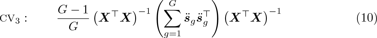
CV₃ can be written in several ways. One of them is

{CV}_{3} : \frac{G - 1}{G} {(X^{⊤} X)}^{- 1} (\sum_{g = 1}^{G} {\ddot{s}}_{g} {\ddot{s}}_{g}^{⊤}) {(X^{⊤} X)}^{- 1}

where the modified score vectors $\ddot{s}$ _g are defined as

{\ddot{s}}_{g} = X_{g}^{⊤} M_{g g}^{- 1} {\hat{u}}_{g}

Here $M_{g g} = I_{N_{g}} - X_{g} {(X^{⊤} X)}^{- 1} X_{g}^{⊤}$ is the diagonal block corresponding to the gth cluster of the projection matrix M_X , which satisfies $\hat{u} = M_{X} u .$ . Although computing CV₃ using (10) works well when all the N_g are very small, it becomes expensive, or perhaps computationally infeasible, when one or more of the N_g is large. The problem is that an N_g × N_g matrix needs to be stored and inverted for every cluster. Niccodemi et al. (2020) propose a method that is much faster for large clusters, versions of which apply to both CV₂ and CV₃. However, recognizing that CV₃ is a jackknife estimator makes a method available that is even simpler and usually faster.

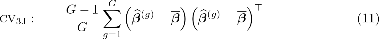
There are actually two cluster jackknife estimators of $Var (\hat{β})$ . The simplest is probably

{CV}_{3 J} : \frac{G - 1}{G} \sum_{g = 1}^{G} ({\hat{β}}^{(g)} - \bar{β}) {({\hat{β}}^{(g)} - \bar{β})}^{⊤}

where $\bar{β}$ is the sample mean of the ${\hat{β}}^{(g)}$ , which were defined in (9). The expression in (11) is the cluster analog of the usual jackknife variance matrix estimator given in MacKinnon and White [1985, (11)]. Each of the ${\hat{β}}^{(g)}$ is obtained by deleting a cluster instead of an observation, and the summation is over clusters instead of observations. If $\bar{β}$ in (11) is replaced by $\hat{β}$ , we instead obtain

{CV}_{3} : \frac{G - 1}{G} \sum_{g = 1}^{G} ({\hat{β}}^{(g)} - \hat{β}) {({\hat{β}}^{(g)} - \hat{β})}^{⊤}

This version of CV₃ is numerically identical to the one in (10) (MacKinnon, Nielsen, and Webb 2023c, sec. 3). Unless all the clusters are very small, computing CV₃ using (12) is much faster than using (10); timings are reported in MacKinnon, Nielsen, and Webb (2023c).

Many discussions of jackknife variance estimation follow Efron (1979) and use $\bar{β}$ as in (11), but others, including Bell and McCaffrey (2002), use $\hat{β}$ as in (12). Although these two jackknife variance estimators are asymptotically the same, they are rarely equal because CV₃ minus CV_3J is a positive semidefinite matrix. In practice, however, they tend to be very similar (MacKinnon, Nielsen, and Webb 2023c), and there seems to be no good reason to expect either CV₃ or CV_3J to perform better in general. Interestingly, the original HC₃ estimator proposed in MacKinnon and White (1985) is actually the analog of CV_3J. The modern version of HC₃, which is the analog of CV₃, seems to be due to Davidson and MacKinnon (1993, chap. 16). This version of HC₃ is normally computed by dividing each residual by the corresponding diagonal element of M_X , and the factor of (N − 1)/N is usually (but incorrectly) omitted.

The factor of (G − 1)/G in both (11) and (12) is designed to compensate for the tendency of the ${\hat{β}}^{(g)}$ to be too spread out. This factor is the analog of the usual factor of (N − 1)/N for a jackknife variance matrix at the individual level. It implicitly assumes that all clusters are the same size and perfectly balanced, with disturbances that are independent and homoskedastic. In this special case, the estimators CV₃ and CV_3J would be identical and unbiased (Bell and McCaffrey 2002). These estimators are already available in Stata. When used with the cluster() option, the vce(jackknife) option computes CV_3J standard errors, and the vce(jackknife, mse) option computes CV₃ standard errors. Because it is specialized for linear regression models, the implementation in summclust is much faster.

Both jackknife estimators may readily be used to compute cluster–robust t statistics. Because there are G terms in the summation, it seems natural to compare these with the t(G − 1) distribution, as usual. These procedures should almost always be more conservative than t tests based on the widely used CV₁ estimator. In an important recent article, Hansen (2022) shows that CV₃ has much better worst-case theoretical properties than CV₁. This strongly suggests that t statistics based on CV₃ are likely to yield lower rejection frequencies than ones based on CV₁. The simulation results in section 7 and in MacKinnon, Nielsen, and Webb (2023c) are consistent with this conjecture.

When a model includes fixed effects, some care must be taken when computing CV₃ and CV_3J. As noted in section 2.1, it is computationally attractive to partial out fixed effects prior to calculating $\hat{β}$ . However, if we were to partial out any arbitrary regressors prior to computing the delete-one-cluster estimates in (9), then the computed ${\hat{β}}^{(g)}$ would depend on the values of the partialed-out regressors for the full sample, including those in the gth cluster. Consequently, the values of CV₃ and CV_3J will be incorrect if we partial out any regressor that affects more than one cluster (such as industry-level fixed effects with firm-level clustering). The regressors that are partialed out must be cluster fixed effects or fixed effects at a finer level (such as firm-level fixed effects with industry-level clustering), because each of them affects only one cluster. See the discussion of the absorb() and fevar() options in section 3.

The vector β can be identified for the full sample but not when one cluster is deleted. For example, consider the coefficient on a dummy variable that takes on nonzero values only for observations in the gth cluster. This coefficient cannot be identified when cluster g is omitted. In such a case, the matrix $X^{⊤} X - X_{g}^{⊤} X_{g}$ in (9) is singular, and CV₃ and CV_3J cannot be computed using an ordinary matrix inverse. However, because summclust uses the invsym() function in Stata, which implements a generalized inverse, the offending element of ${\hat{β}}^{(g)}$ is simply replaced by 0. The command therefore checks whether any of the ${\hat{β}}^{(g)}$ coefficients of interest are equal to 0 and issues a warning when they are; see section 3.

There may be more than one set of fixed effects that are invariant at the cluster level. For example, imagine an analysis of students’ test scores where the researcher wants to control for both school and neighborhood fixed effects and cluster the standard errors at the state level. In this case, neither of Stata’s built-in regress and areg commands can produce an estimate of CV₃ because the fixed effects for schools and neighborhoods in state g cannot be identified when state g is omitted. However, summclust can produce such an estimate.

2.3 What should be reported

We believe that investigators should routinely compute the L_g . They should also compute the L_gj for any coefficients of particular interest. In some cases, the L_g and the L_gj will be roughly proportional to the N_g (the cluster sizes). That in itself would be informative. It may be even more interesting, however, to find that the relative size of L_g or L_gj for some clusters g is much larger or much smaller than the relative size of N_g .

When there are few clusters, it is easy enough to look at all the N_g , ${\hat{β}}_{j}^{(g)}$ , L_g , and L_gj to see whether any clusters are unusually large, are unusually influential, or have unusually high leverage or partial leverage. Once G exceeds 10 or 12, however, it may be more informative to report summary statistics or to plot these quantities. The summclust command always reports the minimum, first quartile, median, mean, third quartile, and maximum of the N_g and the L_g . It also reports these quantities for the L_gj and the ${\hat{β}}_{j}^{(g)}$ for the specified regressor j, and by default it provides a figure containing four scatterplots of the L_g and the L_gj against the N_g and the ${\hat{β}}^{(j)}$ ; see sections 3 and 4.

Another possibility is to report a few summary statistics, as summclust also does. Consider a generic (positive) quantity a_g , which might denote any of N_g , L_g , or L_gj for g = 1,…, G. It seems plausible that inference may be unreliable when any of the a_g vary substantially across clusters, and we provide some evidence to support this conjecture in section 7.

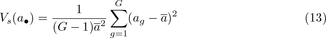
There are many measures of how much the distribution of the a_g differs from what it would be in the perfectly balanced case. One of these is the scaled variance

V_{s} (a_{•}) = \frac{1}{(G - 1) {\bar{a}}^{2}} \sum_{g = 1}^{G} {(a_{g} - \bar{a})}^{2}

where the argument a _• denotes the entire set of a_g for g = 1,…, G and ā denotes the arithmetic mean, which is N/G for the N_g , k/G for the L_g , and 1/G for the L_gj . These are all positive numbers, so it is reasonable to scale by their squares. Larger values of V_s imply that the a_g are more variable across clusters, relative to their mean. We could report either V_s or its square root, which is often called the coefficient of variation. In the perfectly balanced case, V_s = 0. By default, summclust reports the coefficient of variation for the cluster sizes, the leverages, the partial leverages, and the ${\hat{β}}_{j}^{(g)}$ .

Another possibility, although valid only for positive quantities, is to report one or more alternative sample means. The more these differ from the arithmetic mean, the more heterogeneous the clusters must be. Three common alternatives to the arithmetic mean are the harmonic, geometric, and quadratic means:

{\bar{a}}_{harm} = {(\frac{1}{G} \sum_{g = 1}^{G} 1 / a_{g})}^{- 1}, {\bar{a}}_{geo} = {(\prod_{g = 1}^{G} a_{g})}^{1 / G}, and {\bar{a}}_{quad} = {(\frac{1}{G} \sum_{g = 1}^{G} a_{g}^{2})}^{1 / 2}

Unless all the a_g are the same, the harmonic and geometric means will be less than the arithmetic mean ā, and the quadratic mean (which has the same form as the root mean squared error of an estimator) will be greater than ā. summclust optionally reports all three of these alternative means, along with the ratio of each of them to ā. The three ratios provide scale-free measures of cluster heterogeneity; the closer they are to 1, the more homogeneous the clusters are.

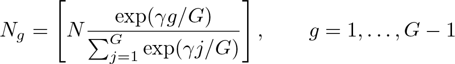
Another way to quantify the heterogeneity of the cluster sizes and the regressors is to calculate G ^∗, the “effective number of clusters,” as proposed in Carter, Schnepel, and Steigerwald (2017). The value of G ^∗ depends on the coefficient j for which it is being computed and on a parameter ρ to be discussed below, so we denote it $G_{j}^{*} (ρ)$ . It is defined as

G_{j}^{*} (ρ) = \frac{G}{1 + Γ_{j} (ρ)}, Γ_{j} (ρ) = \frac{1}{G} \sum_{g = 1}^{G} {\frac{γ_{g j} (ρ) - {\bar{γ}}_{j} (ρ)}{{\bar{γ}}_{j} (ρ)}}^{2}, {\bar{γ}}_{j} (ρ) = \frac{1}{G} \sum_{g = 1}^{G} γ_{g j} (ρ)

where 0 ≤ ρ ≤ 1 and the γ_gj (ρ) are given by

γ_{g j} (ρ) = e_{j}^{⊤} {(X^{⊤} X)}^{- 1} X_{g}^{⊤} Ω_{g} (ρ) X_{g} {(X^{⊤} X)}^{- 1} e_{j}, g = 1, \dots, G

Here e _j is a k-vector with 1 in the jth position and 0 everywhere else, so $e_{j}^{⊤}$ ( X ^⊤ X ) ⁻ ¹ is the jth row of ( X ^⊤ X ) ⁻ ¹, and Ω _g (ρ) is an N_g × N_g matrix with 1 on the principal diagonal and ρ everywhere else. It is easy to see that

Ω_{g} (ρ) = ρ ι ι^{⊤} + (1 - ρ) I

where ι is an N_g -vector of 1s and I is an N_g × N_g identity matrix. Note that Γ _j (ρ) is just the scaled variance of the γ_gj (ρ); compare (13).

The parameter ρ may be interpreted as the intracluster correlation coefficient for a model with cluster-level random effects. Because ρ is unknown, Carter, Schnepel, and Steigerwald (2017) suggest calculating $G_{j}^{*} (1)$ as a sort of worst case. However, when there are cluster-level fixed effects or fixed effects at a finer level nested within clusters, they will absorb all the intracluster correlation. Thus, it does not make sense to specify ρ > 0 in either of these cases. It does seem natural to use $G_{j}^{*} (0)$ , however, because the amount of intracluster correlation that remains in models with cluster fixed effects is often quite small.

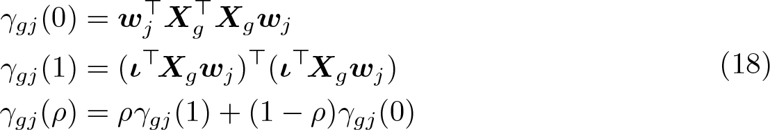
From (15) and (16), we see that

X_{g}^{⊤} Ω_{g} (ρ) X_{g} = ρ {(ι^{⊤} X_{g})}^{⊤} (ι^{⊤} X_{g}) + (1 - ρ) X_{g}^{⊤} X_{g}

This result makes it inexpensive to compute the γ_gj (ρ) for any value of ρ by first computing them for ρ = 0 and ρ = 1. The needed equations are

\begin{array}{l} γ_{g j} (0) = w_{j}^{⊤} X_{g}^{⊤} X_{g} w_{j} \\ γ_{g j} (1) = {(ι^{⊤} X_{g} w_{j})}^{⊤} (ι^{⊤} X_{g} w_{j}) \\ γ_{g j} (ρ) = ρ γ_{g j} (1) + (1 - ρ) γ_{g j} (0) \end{array}

where w _j is the jth column of ( X ^⊤ X ) ⁻ ¹. After we obtain the γ_gj (ρ) from (18), it is trivial to compute $G_{j}^{*} (ρ)$ using (14). Evidently, $G_{j}^{*} (ρ)$ is always less than G. When it is much smaller than G, it can provide a useful warning.

Suppose that we have partialed out cluster fixed effects prior to computing $G_{j}^{*} (ρ)$ . Then the first term on the right-hand side of (17) should theoretically be a zero matrix because every column of X _g should add to zero. In practice, however, the limitations of floating-point arithmetic mean that this matrix will actually contain extremely small positive numbers. This will cause the computation of $G_{j}^{*} (ρ)$ to be numerically unstable. When the fixed effects are not partialed out, similar but more complicated numerical issues arise.

The command clusteff, discussed in Lee and Steigerwald (2018), is designed to calculate $G_{j}^{*} (ρ)$ , with ρ = 0.9999 rather than ρ = 1 by default to avoid numerical instabilities. However, the only version of this command that we have used does so in a computationally inefficient way that does not use (18). When any of the N_g is large, it can take a very long time or even fail because Stata runs out of memory. For example, it failed with some of the samples in MacKinnon, Nielsen, and Webb (2023a).

Like V_s (a _•) and the alternative sample means for measures of leverage and partial leverage discussed above, $G_{j}^{*} (ρ)$ is sensitive not only to variation in cluster sizes but also to other features of the X _g matrices. But it is not sensitive to heteroskedasticity or to any other features of the disturbances. summclust computes $G_{j}^{*} (0), G_{j}^{*} (1)$ , and (optionally) $G_{j}^{*} (ρ)$ for a specified covariate. However, when there are cluster fixed effects, or fixed effects nested within clusters, it computes only $G_{j}^{*} (0)$ . For example, it will not compute $G_{j}^{*} (ρ)$ for ρ ≠ 0 whenever there are state-level fixed effects and clustering at the region level.

The quantity $G_{j}^{*} (0)$ is very closely related to V_s ( L _• _j ), where L _• _j denotes the entire set of L _gj , for g = 1,…, G. The γ_g (0) defined in (15) and (18) are equal to the L_gj defined in (7) divided by ${\dot{x}}_{j}^{⊤} {\dot{x}}_{j}$ . Because this makes the γ_g (0) proportional to the L_gj , V_s (L _• _j ) is numerically identical to Γ(0); compare (13) and the middle equation in (14). Thus, we see from the first equation in (14) that $G_{j}^{*} (0)$ is simply a monotonically decreasing function of the scaled variance of our measures of partial leverage at the cluster level. When V_s (L _• _j ) is large, $G_{j}^{*} (0)$ is necessarily much smaller than G.

3 The summclust command

In this section, we describe the summclust command, which calculates many statistics to help assess cluster heterogeneity and also provides CV₃ and CV_3J standard errors. The command does not rely on any other Stata commands, but it does require a version of Stata that provides Mata’s panelsum() function (version 13 or later).

We first present an overview of the summclust command, followed by a simple illustration using nlswork.dta.

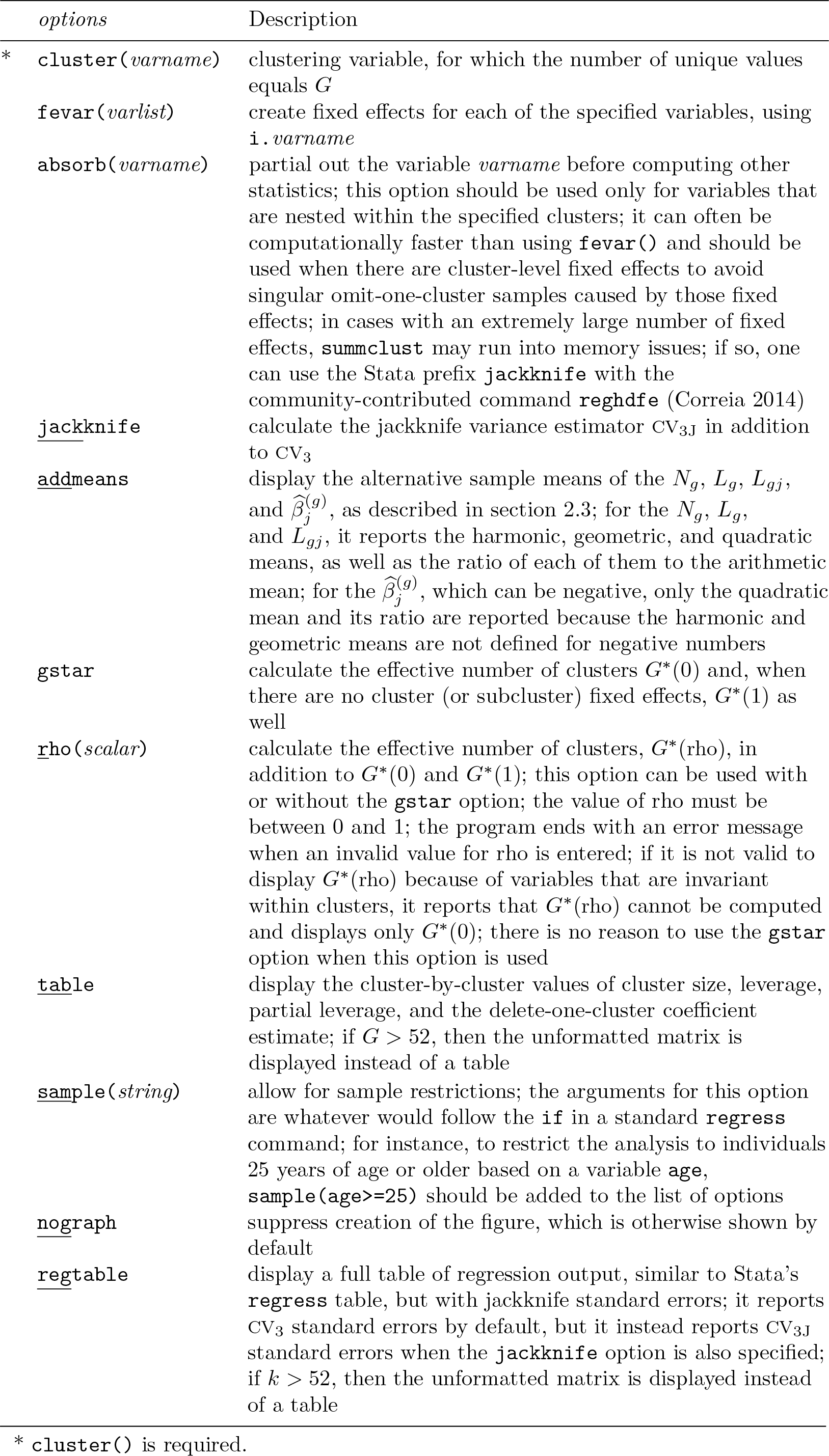
3.1 Syntax and options

3.1.1 Syntax

summclust varlist , cluster( varname ) [options}

varlist specifies the dependent variable, the independent variable of interest, and other (binary or continuous) independent variables. At least one additional regressor must be specified. Time-series operators and factor variables are not permitted.

options	Description
* cluster( varname )	clustering variable, for which the number of unique values equals G
fevar( varlist )	create fixed effects for each of the specified variables, using i. varname
absorb( varname )	partial out the variable varname before computing other statistics; this option should be used only for variables that are nested within the specified clusters; it can often be computationally faster than using fevar() and should be used when there are cluster-level fixed effects to avoid singular omit-one-cluster samples caused by those fixed effects; in cases with an extremely large number of fixed effects, summclust may run into memory issues; if so, one can use the Stata prefix jackknife with the community-contributed command reghdfe (Correia 2014)
jackknife	calculate the jackknife variance estimator CV_3J in addition to CV₃
addmeans	display the alternative sample means of the N_g , L_g , L_gj ,and ${\hat{β}}_{j}^{(g)}$ , as described in section 2.3; for the N_g , L_g ,and L_gj , it reports the harmonic, geometric, and quadratic means, as well as the ratio of each of them to the arithmetic mean; for the ${\hat{β}}_{j}^{(g)}$ , which can be negative, only the quadratic mean and its ratio are reported because the harmonic and geometric means are not defined for negative numbers
gstar	calculate the effective number of clusters G ^∗(0) and, when there are no cluster (or subcluster) fixed effects, G ^∗(1) as well
rho( scalar )	calculate the effective number of clusters, G ^∗(rho), in addition to G ^∗(0) and G ^∗(1); this option can be used with or without the gstar option; the value of rho must be between 0 and 1; the program ends with an error message when an invalid value for rho is entered; if it is not valid to display G ^∗(rho) because of variables that are invariant within clusters, it reports that G ^∗(rho) cannot be computed and displays only G ^∗(0); there is no reason to use the gstar option when this option is used
table	display the cluster-by-cluster values of cluster size, leverage, partial leverage, and the delete-one-cluster coefficient estimate; if G > 52, then the unformatted matrix is displayed instead of a table
sample( string )	allow for sample restrictions; the arguments for this option are whatever would follow the if in a standard regress command; for instance, to restrict the analysis to individuals 25 years of age or older based on a variable age, sample(age>=25) should be added to the list of options
nograph	suppress creation of the figure, which is otherwise shown by default
regtable	display a full table of regression output, similar to Stata’s regress table, but with jackknife standard errors; it reports CV₃ standard errors by default, but it instead reports CV_3J standard errors when the jackknife option is also specified; if k > 52, then the unformatted matrix is displayed instead of a table

* cluster() is required.

3.1.2 Description

summclust is a stand-alone command for summarizing cluster variability in several ways. It always calculates measures of cluster-level influence and leverage, and it optionally calculates the effective number of clusters. It also always reports CV₁ and CV₃ standard errors for one coefficient, and it optionally reports a CV_3J standard error as well. If requested, it can calculate additional measures of cluster-level heterogeneity. Unless it is told not to, it produces a figure that can help identify the source of cluster-level heterogeneity. Finally, it can optionally produce a full table of regression results with CV₃ standard errors.

By default, summclust calculates the CV₃ standard error based on (10). With wellbehaved samples, this should match the standard error calculated using Stata’s native jackknife: regress y x, cluster(group) or regress y x, cluster(group) vce(jackknife) commands. However, many samples are not well behaved, in that the regressor matrices for some of the omit-one-cluster subsamples may not have full rank. We will refer to such subsamples, rather informally, as “singular subsamples”.

Whenever there are singular subsamples, summclust calculates two standard errors. One of these drops the singular subsamples as the native Stata commands do. The other uses a generalized inverse. summclust provides guidance as to which standard error is likely to be more reliable. When regtable is specified and singular subsamples are present, two versions of the regression table are displayed. Similarly, if jackknife is specified and there are singular subsamples, four different standard errors are shown, either CV₃ or CV_3J, combined with either the generalized inverse or one that drops the singular subsamples.

nograph suppresses creation of the figure, which is otherwise shown by default. The figure shows four scatterplots: leverage against observations per cluster, partial leverage against observations per cluster, leverage against omit-one-cluster coefficients, and partial leverage against omit-one-cluster coefficients. This figure can be quite informative, but it is computationally costly to produce. We recommend invoking this option after the figure has been inspected.

When jackknife is specified, regtable uses the CV_3J estimates to produce the regression table. Otherwise, CV₃ estimates are used.

3.2 Illustration with nlswork

To illustrate summclust‘s functionality and syntax, we consider a simple example using nlswork.dta, which contains a sample of women who were 14–26 years of age in 1968 from the National Longitudinal Survey of Young Working Women. For this exercise, we restrict the sample to individuals who are 20 to 40 years old.

We estimate a simple Mincer regression using nlswork.dta to see whether there is a marriage premium for wages. The variable msp is equal to 1 if the person is married and cohabits with their spouse and equal to 0 otherwise. For this example, we cluster by industry. The following code opens the dataset and estimates the regression using Stata’s regress command:

The output from the command above provides CV₁ standard errors. Alternatively, we can estimate CV₃ and CV_3J standard errors using this code:

When either of these commands is run, Stata displays the warning Note: One or more parameters could not be estimated in 2 jackknife replicates; standard-error estimates include only complete replications.

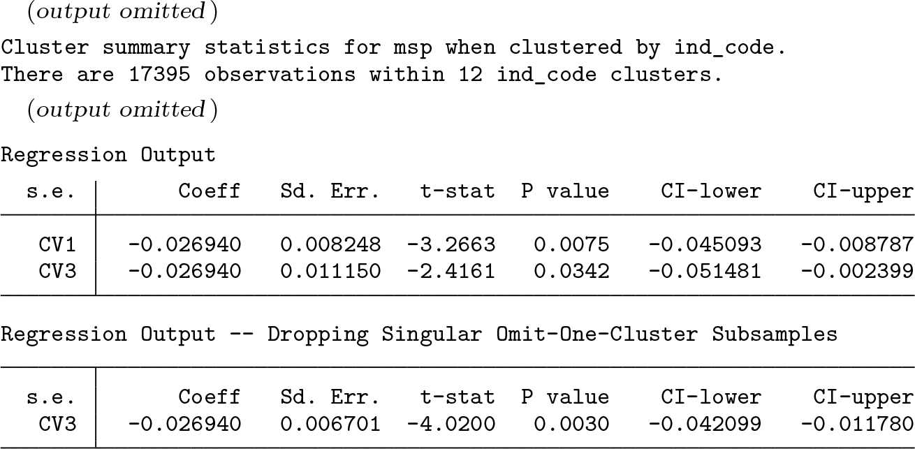
The coefficient on msp and two or three standard errors can also be obtained using summclust. The basic command is

summclust ln_wage msp union race, fevar(grade age birth_yr) cluster(ind)

This code results in the default output from summclust, which is mostly contained in two tables. The first one includes the coefficient on the second variable in the varlist (in this case msp), the CV₁ and CV₃ standard errors for this coefficient, and the associated t statistics, p-values, and confidence intervals. In this case, summclust also displays a warning about singular subsamples and thus produces two Regression Output tables. The standard errors in the table that drops singular subsamples match those produced natively in Stata.

In the first table for this example, the CV₁ and CV₃ standard errors are noticeably different, with the latter being considerably larger. However, in the second table, where the two singular subsamples are dropped, the CV₃ standard error becomes much smaller.

The Cluster Variability table from summclust (below) provides insight into what is happening. It reports summary statistics for N_g , L_g , L_gj , and ${\hat{β}}_{j}^{(g)}$ . Whenever singular subsamples are dropped, two sets of statistics are shown for ${\hat{β}}_{j}^{(g)}$ . The first (second-last column) uses all the jackknife subsamples with a generalized inverse standard error. The second (final column) uses only the nonsingular subsamples. We can see that the largest value of ${\hat{β}}_{j}^{(g)}$ is considerably smaller (and therefore more different from the other values) when none of the subsamples is dropped. This explains why the CV₃ standard error is larger in the first table above than in the second one.

It is evident from this table that the clusters are extremely heterogeneous. The largest cluster contains almost one-third of the sample and is 167 times the size of the smallest. There are also extreme differences in both leverage and partial leverage across clusters. The ratio of the largest to the smallest value is 198 for leverage and 504.5 for partial leverage. The sum of the leverages is 12 × 4.583333 = 55, which is the number of estimated coefficients. Although both sets of ${\hat{β}}_{j}^{(g)}$ vary quite a bit, dropping one cluster never changes the sign of the coefficient.

The option fevar() is used when there are factor variables, which would be specified as i. varname in conventional Stata syntax. In the above example, the arguments to fevar() are grade, age, and birth_yr. For each argument, a set of temporary dummy variables is created. These dummy variables are included in the regression, and there is no constant term if they are present.

The sample code above does not illustrate several additional options. The most important of these is the absorb() option, which operates like fevar(). It treats its argument, a single variable, as an additional factor variable to include in the set of regressors. absorb( varname ) can be used when including i. varname in a regression would result in many fixed effects. Speed can often be increased, perhaps substantially, by partialing out the absorbed fixed effects from the dependent and all the independent variables. It is advisable to use absorb() rather than fevar() whenever their argument corresponds to a set of cluster fixed effects because the elements of ${\hat{β}}^{(g)}$ that correspond to the fixed effects cannot be identified in that case; see section 2.1.

The absorb() option should be used with care. Partialing out fixed effects is valid for the measures of leverage and influence and for the jackknife variance matrices only when the absorbed variable yields fixed effects that can be partialed out on a clusterby-cluster basis. That is, absorb() should be used only for straight cluster fixed effects or for fixed effects at a finer level, such as state × year fixed effects for a panel with clustering at the state level. It is not valid to partial out fixed effects that are not limited to one cluster. In that case, the ${\hat{β}}^{(g)}$ and quantities based on them would be different for the original data and the data after partialing out because the partialed-out observations for the gth cluster would depend on other clusters as well. Accordingly, summclust checks to ensure that the clustering variable is invariant within each value of the absorbed variable. When it is not invariant, a warning is displayed, and the values of L_g , L_gj , ${\hat{β}}_{j}^{(g)}$ , CV₃, and CV_3J are not available.

To see the difference between fevar() and absorb(), we can estimate an expanded regression that includes industry fixed effects. Consider the following two commands:

For the command that uses fevar() for all the categorical variables, some of the output is

Because every one of the jackknife subsamples is singular, only the results based on the generalized inverse are reported. In contrast, when absorb() is used for the industry fixed effects, the corresponding output is instead

These two tables highlight a key reason for using absorb(). Because only two of the jackknife subsamples are singular, summclust can report both standard errors. Observe that when all 12 jackknife samples are used, the standard errors are the same regardless of whether industry fixed effects are specified using fevar() or absorb().

Using the fevar() option leads to the output below for the measures of cluster variability:

Using the absorb() option leads instead to the output below:

The ${\hat{β}}_{j}^{(g)}$ when all clusters are retained are identical for both options. But because there are two singular subclusters, there are two versions of the ${\hat{β}}_{j}^{(g)}$ for the fevar() results.

The leverage estimates are also smaller when we use the absorb() option. Recall that, for the original model with no industry fixed effects, the leverages summed to 55. In the first case just above, where the industry fixed effects are included as regressors in fevar(), the regression has 66 coefficients, and so the leverages sum to 12 × 5.5 = 66. In the second case, where the industry fixed effects are partialed out using absorb(), the regression has 54 coefficients, and so the leverages sum to 12 × 4.5 = 54. Thus, for the first case each of the leverages is greater than the corresponding one for the second case by precisely 1.

3.2.1 Examples

In the examples that follow, we include the nograph option to reduce computational time.

This example illustrates the jackknife and table options:

In addition to the two standard tables, there is the following table:

This table makes it easy to see whether the high leverage clusters are also the largest clusters. That is clearly the case here. After the program runs, this table is stored as the Mata matrix scall.

To obtain summary statistics on the four (or five) measures of cluster variability, we can use the addmeans option:

This command produces the following table:

Once again, we see that there is extreme variability across the clusters. This is particularly noticeable for the ratio of the harmonic mean to the arithmetic mean, which is between 0.060 and 0.143 for the cluster size, leverage, and partial leverage measures. Recall that these ratios would be close to 1 if the clusters were relatively homogeneous. This table is stored in Mata’s memory as bonus.

To obtain estimates of the effective number of clusters, we can use either the gstar option or the rho() option. The former displays $G_{j}^{*} (0)$ and $G_{j}^{*} (1)$ . The latter requires a specified value of ρ and displays $G_{j}^{*} (0)$ and $G_{j}^{*} (1)$ along with $G_{j}^{*} (ρ)$ . When there are fixed effects at the cluster or subcluster level, only $G_{j}^{*} (0)$ is reported.

For the nlswork example, the first option may be called as

This yields

The second option, using ρ = 0.5 as an illustration, may be called as

This yields

In this example, the effective number of clusters is clearly substantially less than the actual number of clusters. This provides more evidence that inference using the CV₁ standard error together with the t(G − 1) distribution is likely to be unreliable. These three quantities can be accessed in Mata’s memory as gstarzero, gstarrho, and gstarone, respectively.

By using the regtable option, one can display a modified version of the regression table that is similar to the default output from Stata’s regress command. The command is

When there are singular subsamples, two versions of this table will be displayed. In this example, the table is quite long, so we do not reproduce it here.

3.3 List of stored results

All the results that are displayed as output can also be found in Mata’s memory. To access one of these after running summclust, simply add the following line:

mata: object_name

The object_name can take one of the following values:

cvstuff: This matrix stores the table with the title Regression Output. It is 2 × 6 when the jackknife option is not used (the default) and 3 × 6 when jackknife is used.

clustsum: The matrix with the measures of cluster variability.

scall: This matrix stores the G × 4 table created by the table option with the title Cluster by Cluster Statistics.

bonus: This 6 × 4 matrix contains the alternative sample means and their ratios to the arithmetic mean created by the addmeans option.

cnames: The string matrix with the cluster names, to match with elements in scall. This matrix is calculated only when the option table is specified.

gstarzero: This scalar contains $G_{j}^{*} (0)$ , created by the gstar or rho() option.

gstarone: This scalar contains $G_{j}^{*} (1)$ , created by the gstar or rho() option.

gstarrho: This scalar contains $G_{j}^{*} (ρ)$ , created by the rho() option.

regresstab: This matrix contains the table shown when the regtable option is specified.

Scalars within matrices can be referenced on a cell-by-cell basis. For example, the CV₃ standard error is stored in the second row and second column of cvstuff, and to display it one can enter the following command:

mata: cvstuff[2,2]

Additionally, several results are available as scalars or matrices in return memory using r(). The available scalars are

The standard error, t statistic, p-value, and confidence interval bounds are also available for the CV₃ and CV_3J standard errors. To access these, replace “1” in the above with either “3” or “3J”; for example, the p-value using CV_3J is available in cv3Jp. In the event of singular subsamples, there are two versions of the CV₃ or CV_3J results. The ones where singular subsamples have been dropped have a suffix of drop. For instance, cv3sedrop is used instead of cv3se.

The available matrices are

4 Empirical example

We consider an empirical example from Busso and Galiani (2019) that studies an experiment where retail firms were randomly assigned to enter one of 72 different geographic markets (mercados in Spanish) within the Dominican Republic. After randomization, 21 markets had no entrants and so were in the control group, 18 had one entrant, another 18 had two, and the remaining 15 had three. The primary analysis distinguishes only between the 51 treated markets and the 21 control markets. The number of observations (stores) per market varies from 20 to 55.

This example is interesting because conventional wisdom (for example, MacKinnon, Nielsen, and Webb [2023a]) suggests that, with 72 clusters that do not vary much in size, and with neither few treated nor few control clusters, inference based on CV₁ standard errors and the t(71) distribution should work well. However, our leverage measures suggest otherwise, and alternative inference methods yield noticeably different results.

The model we fit is

Y_{s d} = α + γ Z_{d} + X_{s d} β + ϵ_{s d}

Here s indexes stores and d indexes markets. The treatment variable Z_d equals 1 if market d is treated (there was entry) and 0 if it was a control (there was no entry). The coefficient of interest is γ, which measures the causal effect of increased competition on an outcome Y . We focus on just one of several outcomes, namely, the log of demeaned prices after treatment. The results from this regression are found in table 5, panel B, column 4, row 1 of Busso and Galiani (2019). The table states that there are 72 clusters and 2,025 observations; however, the replication dataset that we use contains just 1,926 observations.

Regression (19) includes 17 control variables in the row vector X _sd . These are the first lag of the outcome variable, the number of retailers in each district pretreatment, a lagged quality index, eight province fixed effects, the total district beneficiaries of a conditional cash transfer program, the percent beneficiaries of that program, the average income in the market, two market education measures, and a binary indicator for the urban status of the market. Thus, the total number of regressors is 19.

The OLS estimate of γ, its CV₁ standard error, the p-value for a test that γ = 0, and a 0.95 confidence interval are shown in the first row of table 1. Allowing for different numbers of reported digits, these estimates accord with the ones in Busso and Galiani (2019). The estimate of −0.01469 has the expected sign (average prices declined). However, the p-value is just slightly less than 0.05, and the confidence interval barely excludes 0.

Table 1.

Estimates of the treatment effect

Method	$\hat{γ}$	Standard error	p-value	Confidence interval
CV₁	−0.01469	0.007243	0.0461	[−0.02913, −0.00025]
CV₂	−0.01469	0.008078	0.0730	[−0.03080, 0.00142]
CV₃	−0.01469	0.009090	0.1105	[−0.03281, 0.00343]
CV_3J	−0.01469	0.009087	0.1104	[−0.03281, 0.00343]
WRC-C bootstrap	−0.01469		0.0891	[−0.03121, 0.00243]
WCR-S bootstrap	−0.01469		0.0913	[−0.03121, 0.00254]

NOTES: There are N = 1926 observations and G = 72 clusters. The two WCR bootstraps use B = 999,999 and a seed of 56,829,046. WRC-C is the classic WCR bootstrap of Cameron, Gelbach, and Miller (2008), and WCR-S is the “score” variant proposed in MacKinnon, Nielsen, and Webb (2023c). It involves transforming the restricted empirical scores in a way based on the jackknife, but it still uses CV₁. The bootstrap results were obtained using version 4.2.0 of boottest.

We next use the summclust command to calculate the cluster-level characteristics of the model and dataset. Some key ones are reported in table 2. It is evident that cluster sizes are well balanced, varying from 20 to 55, with the first and third quartiles equal to 24 and 27. However, both the leverages L_g and the partial leverages L_g ₁ vary considerably. The former range from 0.1308 to 0.7378, and the latter from 0.0001 to 0.0642. The coefficients of variation are 0.3887 and 1.0598, respectively. The latter is moderately large, although not enormous. The two values of G ^∗ are slightly smaller than G/2, which also suggests that the sample is not well balanced.

Table 2.

Leverage and partial leverage for $\hat{γ}$

Statistic	N_g	Leverage	Partial leverage	${\hat{γ}}^{(g)}$
Minimum	20	0.130842	0.000099	−0.017550
First quartile	24	0.204104	0.003166	−0.015089
Median	26	0.235813	0.009001	−0.014791
Mean	26.75	0.263889	0.013889	−0.014663
Third quartile	27	0.292042	0.020926	−0.014070
Maximum	55	0.737797	0.064242	−0.010723
Coef. of variation	0.21	0.388686	1.059813	0.074061

NOTES: There are N = 1926 observations and G = 72 clusters. The effective numbers of clusters are $G_{γ}^{*} (0)$ = 34.16 and $G_{γ}^{*} (1)$ = 33.33.

The coefficient of variation of the ${\hat{γ}}^{(g)}$ is small because most of them do not vary much. However, the most extreme values are notable. The estimate of γ, which is −0.01469, could be as small as −0.01755 or as large as −0.01072 if just 1 out of the 72 clusters was dropped.

These results suggest that CV₁, the default CRVE, may not be particularly reliable in this case. We therefore consider five alternative procedures. The second, third, and fourth rows of table 1 report the CV₂, CV₃, and CV_3J standard errors, along with the p-values and confidence intervals associated with them. The CV₂ p-value is noticeably larger than the CV₁ one and suggests that the estimate is not significant at the 0.05 level. The CV₃ and CV_3J rows are almost identical. At 0.1105, the CV₃ p-value does not even allow us to reject the null at the 0.10 level. The fifth and six rows of table 1 report two WCR bootstrap p-values and the associated 0.95 confidence intervals. At 0.0891 and 0.0913, these are a bit smaller than the jackknife ones, but they clearly do not allow us to reject the null hypothesis at the 0.05 level.

In view of the reasonably large number of clusters and the fact that cluster sizes do not vary much, the large discrepancy between the results for CV₁ and the other procedures may seem surprising. However, it is not all that surprising when we note how much the leverages and, especially, the partial leverages vary.

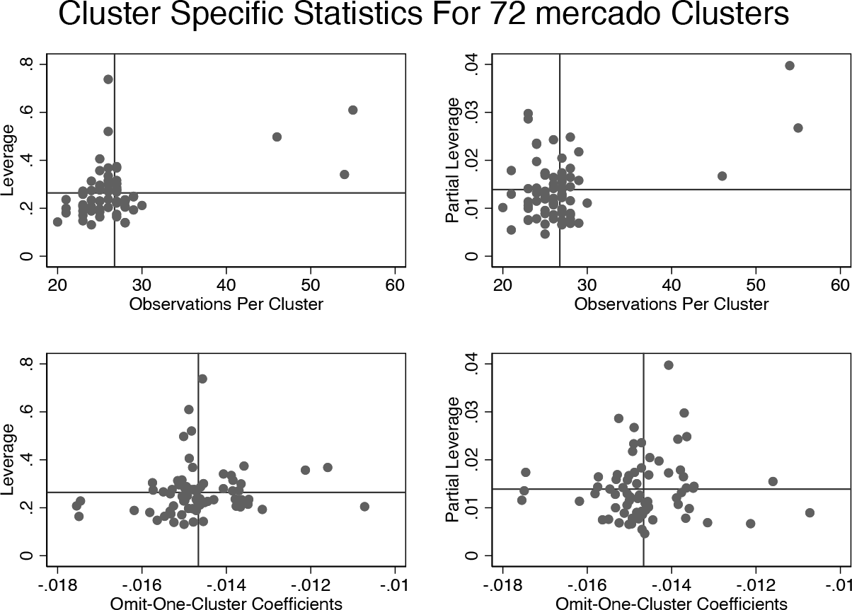
By default, summclust produces a figure like figure 1, with its title created by the program using the name of the clustering variable, in this case mercado. This figure plots both leverage and partial leverage against the number of observations per cluster and also against the omit-one-cluster coefficients. These four subfigures may help to reveal the source of cluster-level heterogeneity. For this example, neither the large leverages nor the large partial leverages come exclusively from clusters with many observations or extreme omit-one-cluster coefficients.

Figure 1.

Example summclust figure.

To explore what is driving the differences in partial leverage, we create an additional scatterplot. Figure 2 plots partial leverage against the number of observations per cluster, with different symbols depending on whether a given market (cluster) was treated. The figure has two interesting features. The first is that the three rather large clusters have fairly small partial leverage. The second is that the 12 clusters with the highest partial leverage are all control markets. The first result is quite surprising because large clusters often have high leverage. But figure 2 makes it clear that there is, in general, no simple relationship between cluster sizes and partial leverage. The second result is not so surprising, because only 21 out of the 72 clusters are controls. Many of the control clusters presumably have high partial leverage because control clusters are relatively rare. See (32) in section 5.4 for an explanation.

Figure 2.

Partial leverage versus cluster size.

5 Simple analytical examples

In this section, we discuss several simple examples in which we can calculate our measures of leverage and influence analytically. These examples are quite revealing.

5.1 Estimation of the mean

Finding the sample mean is equivalent to performing a least-squares regression in which the only regressor is x_i = 1 for all i = 1,…, N. In this case, it is easy to see that $X_{q}^{⊤} X_{g}$ = N_g and X ^⊤ X = N. Therefore,

L_{g} = Tr (H_{g}) = \frac{N_{g}}{N} = \frac{N_{g}}{\sum_{h = 1}^{G} N_{h}}

In this simple case, cluster leverage is exactly proportional to cluster size. In other cases, we can interpret leverage as a generalization of cluster size that also accounts for other types of heterogeneity.

Evidently, $\hat{β} = \bar{y} = N^{- 1} \sum_{g = 1}^{G} N_{g} {\bar{y}}_{g}$ , where $\bar{y}$ and $\bar{y}$ _g denote the sample average for the full sample and for cluster g, respectively. This expression can be rewritten as

\hat{β} = \sum_{g = 1}^{G} \frac{N_{g}}{N} {\bar{y}}_{g} = \sum_{g = 1}^{G} L_{g} {\hat{β}}_{g}

so that $\hat{β}$ is seen to be a weighted average of the G estimates ${\hat{β}}_{g}$ = $\bar{y}$ _g , with the weight for each cluster equal to its leverage. Similarly, we find that

{\hat{β}}^{(g)} = \frac{N}{N - N_{g}} \sum_{h \neq g} L_{h} {\hat{β}}_{h}

where the first factor simply makes up for the fact that we are summing over G − 1 clusters instead of G as in (21). Subtracting (21) from (22), we conclude that

{\hat{β}}^{(g)} - \hat{β} = \frac{N_{g}}{N} ({\hat{β}}^{(g)} - {\hat{β}}_{g}) = L_{g} ({\hat{β}}^{(g)} - {\hat{β}}_{g})

Therefore, cluster g will be influential whenever omitting it yields an estimate ${\hat{β}}^{(g)}$ that differs substantially from the estimate ${\hat{β}}_{g}$ for cluster g itself, especially when cluster g also has high leverage.

5.2 Single regressor plus constant

Consider a regression design with one regressor, x_i , and a constant term. Then

X_{g}^{⊤} X_{g} = [\begin{matrix} N_{g} & \sum_{i = 1}^{N_{g}} x_{g, i} \\ \sum_{i = 1}^{N_{g}} x_{g, i} & \sum_{i = 1}^{N_{g}} x_{g, i}^{2} \end{matrix}], {(X^{⊤} X)}^{- 1} = \frac{1}{N^{2} {\hat{σ}}_{x}^{2}} [\begin{matrix} \sum_{i = 1}^{N} x_{i}^{2} & - \sum_{i = 1}^{N} x_{i} \\ - \sum_{i = 1}^{N} x_{i} & N \end{matrix}]

where ${\hat{σ}}_{x}^{2}$ denotes the sample variance of the x_i . After some algebra, we find that

L_{g} = \frac{N_{g}}{N {\hat{σ}}_{x}^{2}} {{\hat{σ}}_{x}^{2} + {\hat{σ}}_{x, g}^{2} + {({\bar{x}}_{g} - \bar{x})}^{2}}

where $\bar{x}$ _g and ${\hat{σ}}_{x, g}^{2}$ denote the sample mean and sample variance of the x_i within cluster g. Expression (24) is a straightforward generalization of (20). The last two terms within the large braces are the sample variance of the x_g,i within cluster g and the square of the difference between $\bar{x}$ _g and $\bar{x}$ . The sum of these terms is the sample variance of the x_g,i around $\bar{x}$ within cluster g. Thus, cluster g will have high leverage when the variance of the x_g,i around $\bar{x}$ within that cluster is large relative to the variance ${\hat{σ}}_{x}^{2}$ for the full sample. If everything except cluster sizes were perfectly balanced, L_g would evidently reduce to 2N_g/N.

The partial leverage for x is just

L_{g 2} = \frac{N_{g} {{\hat{σ}}_{x, g}^{2} + {({\bar{x}}_{g} - \bar{x})}^{2}}}{N {\hat{σ}}_{x}^{2}}

the total variation around $\bar{x}$ within cluster g divided by the total variation within the sample. If everything except cluster sizes were perfectly balanced, it would reduce to N_g/N.

5.3 One regressor plus fixed effects

Suppose there is one regressor, x_i , and there are cluster-level fixed effects, which have been partialed out. In this case, we can write all quantities as deviations from their cluster averages, and there is no distinction between leverage and partial leverage. Then ${\tilde{X}}_{g}^{⊤} {\tilde{X}}_{g} = \sum_{i = 1}^{N_{g}} {(x_{g, i} - {\bar{x}}_{g})}^{2} = N_{g} {\hat{σ}}_{x, g}^{2} .$ Similarly, ${\tilde{X}}^{⊤} \tilde{X} = \sum_{g = 1}^{G} N_{g} {\hat{σ}}_{x, g}^{2}$ is the average variance of the x_i across all clusters. We find that

L_{g} = \frac{N_{g} {\hat{σ}}_{x, g}^{2}}{\sum_{h = 1}^{G} N_{h} {\hat{σ}}_{x, h}^{2}}

which is again a straightforward generalization of (20). The leverage of cluster g is proportional to N_g times the variance of the x_g,i around $\bar{x}$ _g . Thus, for example, doubling the variance of the x_g,i has the same effect on leverage as doubling N_g .

In this case, using (26), we easily see that

\hat{β} = \frac{\sum_{g = 1}^{G} N_{g} {\hat{σ}}_{x y, g}}{\sum_{g = 1}^{G} N_{g} {\hat{σ}}_{x, g}^{2}} = \sum_{g = 1}^{G} L_{g} \frac{{\hat{σ}}_{x y, g}}{{\hat{σ}}_{x, g}^{2}} = \sum_{g = 1}^{G} L_{g} {\hat{β}}_{g}

where ${\hat{σ}}_{x y, g} = (1 / N_{g}) \sum_{i = 1}^{N_{g}} (x_{g, i} - {\bar{x}}_{g}) (y_{g, i} - {\bar{y}}_{g})$ is the sample covariance of x_i and y_i within cluster g. The rightmost expressions in (21) and (27) are identical. In both cases, $\hat{β}$ is seen to be a weighted average of the G cluster estimates, with the weight for each cluster equal to its leverage.

When cluster g is omitted, we obtain

{\hat{β}}^{(g)} = \frac{\sum_{h \neq g} N_{h} {\hat{σ}}_{x y, h}}{\sum_{h \neq g} N_{h} {\hat{σ}}_{x, h}^{2}} = \frac{\sum_{h \neq g} L_{h} {\hat{β}}_{h}}{\sum_{h \neq g} L_{h}}

which would specialize to (22) if (20) were true. As before, ${\hat{β}}^{(g)}$ is a weighted average of the ${\hat{β}}_{h}$ , with weights proportional to the L_g , which in this case are also the partial leverages. Subtracting (27) from (28), we find that

{\hat{β}}^{(g)} - \hat{β} = L_{g} ({\hat{β}}^{(g)} - {\hat{β}}_{g})

which is formally identical to the rightmost expression in (23), although of course L_g is defined in (26), not (20). Cluster g will be influential whenever ${\hat{β}}^{(g)}$ differs substantially from the estimate ${\hat{β}}_{g}$ for cluster g itself, especially when cluster g also has high leverage.

5.4 Treatment model with a constant term

Now we specialize section 5.2 to the case in which the single regressor is a treatment dummy denoted by d_i . Let $\bar{d}$ _g and $\bar{d}$ denote the proportion of treated observations in cluster g and in the sample, respectively. Then (24) becomes

L_{g} = \frac{N_{g}}{N} (\frac{{\bar{d}}_{g}}{\bar{d}} + \frac{1 - {\bar{d}}_{g}}{1 - \bar{d}})

The first factor here is the relative size of the gth cluster. The second factor depends on how much $\bar{d}$ _g differs from $\bar{d}$ . When $\bar{d}$ _g = $\bar{d}$ , we see that L_g = 2N_g/N. Otherwise, the first term inside the parentheses causes leverage to be high whenever $\bar{d}$ _g is large relative to $\bar{d}$ , and the second term causes leverage to be high whenever $\bar{d}$ _g is small relative to $\bar{d}$ . As d increases for a given $\bar{d}$ _g , the first term becomes smaller relative to the second term. Thus, the gth cluster will tend to be influential when it has either a large proportion of treated observations and the overall proportion is small or a small proportion of treated observations and the overall proportion is large.

We can also obtain the partial leverage of the treatment dummy for this case. Expression (25) simply becomes

L_{g 2} = \frac{N_{g}}{N} (\frac{{\bar{d}}_{g}}{\bar{d}} + \frac{\bar{d} - {\bar{d}}_{g}}{1 - \bar{d}})

Once again, the first factor is the relative size of the gth cluster. The second factor reduces to 1 when $\bar{d}$ _g = $\bar{d}$ , so that L_g ₂ = N_g/N in that special case.

We can further specialize (30) and (31) to models in which the treatment is applied at the cluster level. Suppose that all observations in clusters g = 1,…, G ₁ are treated and no observations in the G ₀ = G − G ₁ control clusters from G ₁ + 1 to G are treated. Then we find that $\bar{d}$ _g = 1 for g = 1,…, G ₁ and $\bar{d}$ _g = 0 for g = G ₁ + 1,…, G. Inserting these into (30) shows that

L_{g} = {\begin{cases} \frac{N_{g}}{N} \frac{1}{\bar{d}} for g = 1, \dots, G_{1}, \\ \frac{N_{g}}{N} \frac{1}{1 - \bar{d}} for g = G_{1} + 1, \dots, G \end{cases}

Inserting them into (31) shows that

\begin{array}{l} L_{g 2} = {\begin{cases} \frac{N_{g}}{N} \frac{\bar{d} + 1}{\bar{d}} for g = 1, \dots, G_{1}, \\ \frac{N_{g}}{N} \frac{\bar{d}}{1 - \bar{d}} for g = G_{1} + 1, \dots, G \end{cases} \end{array}

Thus, any cluster tends to have high leverage if N_g/N is large. A treated cluster has high leverage and partial leverage if $\bar{d}$ is small. Conversely, a control cluster has high leverage and partial leverage if $\bar{d}$ is large.

5.5 Treatment with fixed effects

Finally, we consider the case of cluster-level fixed effects, where treatment is randomly applied at the individual level. This is a special case of section 5.3. We cannot consider cluster fixed effects with cluster-level treatment, because the treatment dummy would be invariant within clusters. We specialize (26) and find that

L_{g} = \frac{N_{g} {\bar{d}}_{g} (1 - {\bar{d}}_{g})}{\sum_{h = 1}^{G} N_{h} {\bar{d}}_{h} (1 - {\bar{d}}_{h})}

Thus, as before, the leverage of cluster g, relative to the average for the other clusters, is proportional to its size, N_g . It also depends on the proportion of treated observations in the cluster. The maximum (relative) leverage for cluster g occurs at $\bar{d}$ _g = 1/2 and is symmetric around 1/2. The result (29) continues to hold. It tells us that cluster g will be influential when its leverage (33) is large and ${\hat{β}}^{(g)}$ differs greatly from ${\hat{β}}_{g}$ .

6 Two-way clustering

Up to this point, we have focused on one-way clustering. However, it is also important to compute measures of leverage, partial leverage, and influence when there is clustering in two or more dimensions (Cameron, Gelbach, and Miller 2011). In the simplest and most commonly encountered case, where there is two-way clustering, we recommend computing the usual one-way measures of leverage, partial leverage, and influence for each of the two clustering dimensions. This requires calling summclust twice.

When the number of clusters in either dimension is small or when the data are seriously unbalanced in either dimension, conventional inference based on a two-way version of CV₁, together with the t min(G − 1, H − 1) distribution, can be seriously unreliable. MacKinnon, Nielsen, and Webb (2021) therefore suggest using the usual two-way CV₁ estimator and applying the original WCR bootstrap to the dimension with the fewest clusters or the most unbalanced clusters. Simulation evidence suggests that this often provides more reliable inferences than the t distribution, but these inferences may still be problematic.

It may also be interesting to calculate measures of leverage, partial leverage, and influence for the intersection of the two clustering dimensions, especially when the number of nonempty intersections is not large. This means calling summclust a third time. Suppose there are two clustering dimensions, with G clusters in the first dimension and H clusters in the second. Then the number of intersection clusters is at most GH , but it can be smaller if some of the intersection clusters are empty. To use summclust for the intersections, we must create a new variable that uniquely identifies each nonempty intersection cluster. Running summclust for this case may be expensive when the number of nonempty intersections is large, especially if k is also large.

Note that, when summclust is invoked three times for each of two clustering dimensions and their intersection, the CV₃ standard error that it reports for each of the three cases is based on a different pattern of one-way clustering. When two-way clustering is appropriate, none of these standard errors is valid. However, what summclust reports can be used to compute an asymptotically valid variance as

{\hat{Var}}_{2 W} ({\hat{β}}_{j}) = {\hat{Var}}_{G} ({\hat{β}}_{j}) + {\hat{Var}}_{H} ({\hat{β}}_{j}) - {\hat{Var}}_{G H} ({\hat{β}}_{j})

Here ${\hat{β}}_{j}$ is the OLS estimate of a coefficient of interest, and the three estimated variances on the right-hand side of (34) are the squares of the CV₃ or CV_3J standard errors reported by summclust for clustering dimension G, clustering dimension H, and the intersection of the two clustering dimensions, respectively.

Asymptotically, the two-way variance Var_2W $({\hat{β}}_{j})$ should not be less than either of the one-way variances. Therefore, if ${\hat{Var}}_{2 W} ({\hat{β}}_{j})$ is less than either ${\hat{Var}}_{G} ({\hat{β}}_{j})$ or ${\hat{Var}}_{H} ({\hat{β}}_{j})$ , it makes sense to replace it by the larger of those two variance estimates. Doing this also eliminates the risk of having to take the square root of a negative number. The appropriate t distribution has min(G−1, H −1) degrees of freedom if ${\hat{Var}}_{2 W} ({\hat{β}}_{j})$ Is used and G − 1 or H − 1 degrees of freedom if it is replaced by either ${\hat{Var}}_{G} ({\hat{β}}_{j})$ or ${\hat{Var}}_{H} ({\hat{β}}_{j})$ , respectively. We conjecture that, especially when this is done, the two-way standard error based on either jackknife estimator will yield more conservative, and generally more reliable, inferences than the usual two-way standard error based on CV₁.

As we discuss in section 3, it is often invalid to partial out fixed effects when computing a jackknife CRVE. This can be particularly tricky in the case of two-way clustering. For example, suppose there are G states and H years. Then it may be desirable to partial out the state fixed effects when computing ${\hat{Var}}_{G} ({\hat{β}}_{j})$ but invalid to partial out the year fixed effects. Similarly, it may be desirable to partial out the year fixed effects when computing ${\hat{Var}}_{H} ({\hat{β}}_{j})$ but invalid to partial out the state fixed effects. Finally, it is invalid to partial out either set of fixed effects when computing ${\hat{Var}}_{G H} ({\hat{β}}_{j})$ . The absorb() option of summclust normally detects cases where partialing out is invalid and refuses to display jackknife standard errors and several other quantities.

7 Simulation experiments

One of the reasons for calculating leverages and partial leverages is to identify cases in which inference may be problematic. The objective of the simulation experiments in this section is to see whether the rejection frequencies for cluster–robust t tests can be predicted from the features of the X matrix reported by summclust. There are 3,000 cases, each corresponding to a particular X matrix. For each case, we generate 10,000 values of y and use them to estimate rejection frequencies for t tests or bootstrap tests at the 0.05 level.

In the experiments, there are either 20 clusters and 2,000 observations or 30 clusters and 3,000 observations. The cluster sizes N_g are determined by a parameter γ ≥ 0, as follows:

N_{g} = [N \frac{\exp (γ g / G)}{\sum_{j = 1}^{G} \exp (γ j / G)}], g = 1, \dots, G - 1

Here [·] denotes the integer part of its argument, and $N_{G} = N - \sum_{j = 1}^{G - 1} N_{g}$ As γ increases, the cluster sizes become increasingly unbalanced. The value of γ is chosen randomly from the U[2, 4] distribution, so the cluster sizes tend to greatly vary. When G = 20, the smallest cluster has between 8 and 32 observations, and the largest has between 229 and 378. When G = 30, the smallest cluster has between 7 and 32 observations, and the largest has between 237 and 396.

There are five regressors, one of which is the test regressor, plus a constant term. The regressors equal either 0 or 1. With probability 1 − p_c , all the observations in a cluster are 0. With probability p_c , they randomly equal either 0 or 1, both with probability 0.5. Thus, when p_c = 1, all variation is at the individual level, and leverage tends to be proportional to cluster sizes. As p_c declines, the samples become more unbalanced. In the experiments, the values of p_c are chosen to be 0.25, 0.30, 0.35, 0.40, 0.50, and 0.60, each for one-sixth of the cases. Smaller values of p_c tend to be associated with larger discrepancies between actual rejection frequencies and 0.05, the nominal level of the tests.

For each experiment, we obtain 12,000 estimated rejection frequencies. One-quarter of these are based on CV₁ and the t(G − 1) distribution, one-quarter on CV₃ and the t(G − 1) distribution, and one-quarter on each of the WRC-C and WCR-S bootstraps. To predict these rejection frequencies, we use a generalized additive model based on smoothing splines; see James et al. (2021, sec. 7.7). The base model can be written as

r_{i} = β_{0} + f_{1} (V_{s i}) + f_{2} (V_{s i}^{1 / 2}) + β_{1} G_{i 0}^{*} + u_{i}

where r_i is the rejection frequency for case i. Here V_si denotes V_s (L _• _j ), the scaled variance of the partial leverages L_gj for the test regressor for case i, $G_{i 0}^{*}$ denotes $G_{j}^{*} (0)$ for the test regressor for case i (recall from section 2.3 that it is a monotonically decreasing function of the L_gj ), and f ₁(·) and f ₂(·) are smoothing splines with five degrees of freedom. Because everything on the right-hand side of (35) is a function of V_si , this model is simply using the V_si to predict the r_i in a potentially nonlinear way.

Figure 3 shows the fitted values from (35), which are predicted rejection frequencies, plotted against the scaled variance of the partial leverages L_gj for four methods of inference and two sample sizes. Panel (a) shows them for t tests based on both CV₁ (solid lines) and CV₃ (dashed lines) for G = 20 and G = 30, and panel (b) shows them for WRC-C and WCR-S bootstrap tests for the same two cases. The model seems to fit quite well, at least for the asymptotic tests, as can be seen from the values of R ² reported for each of the curves. It also fits well for the bootstrap tests, and in fact it has smaller residuals for them than for the asymptotic tests. The lower R ² values for the bootstrap tests simply reflect the fact that there is much less variation to explain.

Figure 3.

Predicted rejection frequencies for asymptotic and bootstrap tests at 0.05 level.

We can see from figure 3 that t tests based on CV₁ often overreject to an extreme degree. For the very smallest values of V_s (L _• _j ), the tests tend to overreject modestly, with predicted rejection frequencies of 0.058 for G = 20 and 0.055 for G = 30. However, these then rise quite rapidly and almost linearly. For G = 30, there are four cases (out of 3,000) for which V_s (L _• _j ) > 15. These are not shown in the figure, but the approximately linear relationship continues to hold, and the fit for these extreme cases is reasonably good.

In contrast, the t tests based on CV₃ tend to underreject for small values of V_s (L _• _j ). For the very smallest values, the predicted rejection frequencies are 0.033 for G = 20 and 0.039 for G = 30. Although it is not obvious from the figure, the CV₃ tests are predicted to underreject somewhat more than half the time, because, in our experiments, most values of V_s (L _• _j ) are quite small. As V_s (L _• _j ) increases, rejection frequencies increase, although for G = 20 they start to decline again once V_s (L _• _j ) exceeds about 9.6. The predicted rejection frequencies never exceed 0.105 for G = 20 and 0.118 for G = 30. In a few cases (74 for G = 20 and 5 for G = 30), the matrix that is inverted in (9) was singular for at least one omit-one-cluster subsample. This happened whenever one of the regressors took the same value for all observations in G − 1 of the clusters. These cases were dropped.

Panel (b) of figure 3 shows the fitted values from (35) for WRC-C and WCR-S bootstrap t tests plotted against the scaled variance of the L_gj . Notice that the scale of the vertical axis differs greatly from the one in Panel (a). All tests, especially the WCR-S ones, perform quite well for smaller values of V_s (L _• _j ). Except for WCR-S with G = 30, however, the rejection-frequency curves are not even close to being linear. This is also the only case for which the fitted values do not deviate greatly from 0.05 for large values of V_s (L _• _j ). In every other case, a large value of V_s (L _• _j ) tends to be associated with substantial levels of overrejection or underrejection.

It is natural to ask whether we can improve the fit of (35) by adding additional explanatory variables that are not simply functions of the V_s (L _• _j ). The answer is that we can. In particular, the variables $\bar{a}$ _geo(L _• _j ) and $G_{j}^{*} (1)$ are often significant when they are added. However, the spline f ₁(V_si ) always remains highly significant, even when many other regressors are included. Thus, at least in these experiments, the scaled variance of the partial leverages, which is the square of their coefficient of variation, seems to be particularly revealing.

Based on these results, which are of course extremely dependent on the way in which the regressors are generated, it seems sensible for investigators to look at several different summary measures for both leverage and partial leverage. That is why summclust reports several of them. In this case, the most informative summary measure appears to be the scaled variance, defined in (13), of the partial leverage measures L_gj , defined in (7), for the regressor of interest. summclust reports the square root of this in the coefvar line of the Cluster Variability table. In general, cluster–robust inference seems to be most reliable when the partial leverages do not vary greatly across clusters.

8 Conclusions

We have discussed a new command, summclust, that is designed to summarize the cluster structure of the dataset for a linear regression model with clustered disturbances. Because the key unit of observation is the cluster, it makes sense to examine measures of influence, leverage, and partial leverage at the cluster level. These are easy to compute and are conceptually very similar to the corresponding classic measures at the observation level (Belsley, Kuh, and Welsch 1980; Chatterjee and Hadi 1986). The summclust command calculates all of them and also reports several summary statistics.

Our measure of influence at the cluster level can provide valuable information about how empirical results depend on the data in the various clusters. Investigators should be wary if dropping one or two clusters changes the results dramatically. However, apart from such cases, the most interesting quantities that summclust calculates generally seem to be the partial leverages and measures that summarize their distribution.

It has long been known that cluster–robust inference can be unreliable when the number of clusters is small. More recent work, including MacKinnon and Webb (2017b, 2018) and Djogbenou, MacKinnon, and Nielsen (2019), has shown that it can also be severely unreliable when cluster sizes vary a lot or when few clusters are treated in the context of difference-in-differences and other treatment models. In both of these cases, leverage and partial leverage tend to vary greatly across clusters. It therefore seems natural to use our measures of leverage and partial leverage as diagnostic tools to identify datasets and regression designs in which cluster–robust inference is likely to be challenging. Simulation results in section 7 suggest that the extent to which partial leverage varies across clusters can be particularly informative. We believe that investigators should always look at the summary statistics reported by summclust and exercise caution whenever they indicate substantial variation across clusters.

As we discussed in section 2.2, the computations needed for leverage and influence are very similar to the ones needed to compute cluster jackknife variance matrix estimators. The summclust command therefore computes two very similar jackknife estimators, which we refer to as CV₃ and CV_3J, almost as a by-product of other computations. These are the same estimators that Stata can produce using the vce(jackknife, mse) and vce(jackknife) options. However, because summclust is designed explicitly for linear regression models fit by OLS, it is faster than using these vce options. Moreover, when summclust is already being used to obtain cluster-level measures of influence and leverage for diagnostic purposes, the additional cost of computing the jackknife variance estimators is minimal.

When the number of clusters is reasonably large and the variation of leverage and partial leverage across clusters is small, we would expect conventional inference based on CV₁ standard errors to perform well. If so, the CV₃ standard errors reported by summclust should be very similar to the CV₁ standard errors reported by one of Stata’s regression commands. When this is the case, there is probably no need for investigators to worry further about the reliability of their inferences. In many cases, however, the CV₃ and CV₁ standard errors will differ noticeably. This happens for the empirical example in section 4, where there are 72 clusters but partial leverage varies a lot. In such cases, the CV₃ standard errors are almost certain to be more conservative and are very likely to be more reliable than the CV₁ ones.

p-values and confidence intervals that are even more reliable can often be obtained by using the restricted wild cluster bootstrap, which is implemented natively with wildbootstrap in Stata 18 and in the package boottest (Roodman et al. 2019). Recent versions of that package implement the WCR-S bootstrap (MacKinnon, Nielsen, and Webb 2023c) in addition to the classic WRC-C bootstrap. We strongly recommend that both variants be calculated whenever the CV₃ and CV₁ standard errors disagree. When the two bootstrap p-values agree, as they do for the empirical example in section 4, then it is probably safe to rely on either of them. When they disagree, then neither of them may be entirely reliable, but we would be inclined to use the one given by the WCR-S bootstrap.

Up to this point, everything in this section has been based on the assumption that there is one-way clustering with a known clustering structure. When more than one level of clustering is plausible, investigators need to choose among them, and this can be challenging; see the discussions in MacKinnon, Nielsen, and Webb (2023a,b). The measures of leverage and influence produced by summclust may be helpful in deciding at what level to cluster.

The current version of summclust is not explicitly designed to handle two-way clustering. However, as we discussed in section 6, it can be called for each clustering dimension to produce two sets of diagnostic statistics. If it is called three times, once for each dimension and once for their intersection, then it can also be used to compute two-way cluster jackknife variance matrix estimators. At present, however, little is known about the properties of these estimators.

10 Programs and supplemental material

Supplemental Material, sj-zip-1-stj-10.1177_1536867X231212433 - Leverage, influence, and the jackknife in clustered regression models: Reliable inference using summclust

Supplemental Material, sj-zip-1-stj-10.1177_1536867X231212433 for Leverage, influence, and the jackknife in clustered regression models: Reliable inference using summclust by James G. MacKinnon, Morten Ørregaard Nielsen and Matthew D. Webb in The Stata Journal

Footnotes

9 Acknowledgments

We are grateful to the editor, an anonymous referee, Alexander Fischer, Raphaël Langevin, and seminar participants at York University, the 2022 Meeting of the Atlantic Canada Economic Association, and the 2022 and 2023 CEA Annual Meetings for comments. We are especially grateful to David Drukker for a very insightful suggestion. MacKinnon and Webb thank the Social Sciences and Humanities Research Council of Canada for financial support (SSHRC grants 435-2016-0871 and 435-2021-0396). Nielsen thanks the Danish National Research Foundation for financial support (DNRF Chair grant number DNRF154).

10 Programs and supplemental material

To install the software files as they exist at the time of publication of this article, type

The command summclust can be installed from the Statistical Software Components archive by typing

or from GitHub by typing

References

Bell

R. M.

McCaffrey

D. F.

. 2002. Bias reduction in standard errors for linear regression with multi-stage samples. Survey Methodology 28: 169–181.

Belsley

D. A.

Kuh

Welsch

R. E.

. 1980 . Regression Diagnostics: Identifying Influential Data and Sources of Collinearity. New York: Wiley. https://doi.org/10.1002/0471725153.

Bester

C. A.

Conley

T. G.

Hansen

C. B.

. 2011. Inference with dependent data using cluster covariance estimators. Journal of Econometrics 165: 137–151. https://doi.org/10.1016/j.jeconom.2011.01.007.

Broderick

Giordano

Meager

. 2023. An automatic finite-sample robustness metric: When can dropping a little data change conclusions? arXiv:2011.14999 [stat.ME]. https://doi.org/10.48550/arXiv.2011.14999.

Busso

Galiani

. 2019. The causal effect of competition on prices and quality: Evidence from a field experiment. American Economic Journal: Applied Economics 11: 33–56. https://doi.org/10.1257/app.20150310.

Cameron

A. C.

Gelbach

J. B.

Miller

D. L.

. 2008. Bootstrap-based improvements for inference with clustered errors. Review of Economics and Statistics 90: 414–427. https://doi.org/10.1162/rest.90.3.414.

Cameron

A. C.

Gelbach

J. B.

Miller

D. L.

. 2011. Robust inference with multiway clustering. Journal of Business and Economic Statistics 29: 238–249. https://doi.org/10.1198/jbes.2010.07136.

Cameron

A. C.

Miller

D. L.

. 2015. A practitioner’s guide to cluster–robust inference. Journal of Human Resources 50: 317–372. https://doi.org/10.3368/jhr.50.2.317.

Carter

A. V.

Schnepel

K. T.

Steigerwald

D. G.

. 2017. Asymptotic behavior of a t-test robust to cluster heterogeneity. Review of Economics and Statistics 99: 698–709. https://doi.org/10.1162/REST_a_00639.

10.

Chatterjee

Hadi

A. S.

. 1986. Influential observations, high-leverage points, and outliers in linear regression. Statistical Science 1: 379–393. https://doi.org/10.1214/ss/1177013622.

11.

Chesher

. 1989. Hájek inequalities, measures of leverage and the size of heteroskedasticity robust Wald tests. Econometrica 57: 971–977. https://doi.org/10.2307/1913779.

12.

Conley

T. G.

Gonçalves

Hansen

C. B.

. 2018. Inference with dependent data in accounting and finance applications. Journal of Accounting Research 56: 1139–1203. https://doi.org/10.1111/1475-679X.12219.

13.

Cook

R. D.

Weisberg

. 1980. Characterizations of an empirical influence function for detecting influential cases in regression. Technometrics 22: 495–508. https://doi.org/10.2307/1268187.

14.

Correia

. 2014. reghdfe: Stata module to perform linear or instrumental-variable regression absorbing any number of high-dimensional fixed effects. Statistical Software Components S457874, Department of Economics, Boston College https://ideas.repec.org/c/boc/bocode/s457874.html.

15.

Davidson

MacKinnon

J. G.

. 1993. Estimation and Inference in Econometrics. New York: Oxford University Press.

16.

Djogbenou

A. A.

MacKinnon

J. G.

Nielsen

M. Ø.

. 2019. Asymptotic theory and wild bootstrap inference with clustered errors. Journal of Econometrics 212: 393–412. https://doi.org/10.1016/j.jeconom.2019.04.035.

17.

Efron

. 1979. Bootstrapping methods: Another look at the jackknife. Annals of Statistics 7: 1–26. https://doi.org/10.1214/aos/1176344552.

18.

Hansen

B. E

. 2022. Jackknife standard errors for clustered regression. Working paper, University of Wisconsin.

19.

Hansen

B. E.

Lee

. 2019. Asymptotic theory for clustered samples. Journal of Econometrics 210: 268–290. https://doi.org/10.1016/j.jeconom.2019.02.001.

20.

Imbens

G. W.

Kolesár

. 2016. Robust standard errors in small samples: Some practical advice. Review of Economics and Statistics 98: 701–712. https://doi.org/10.1162/REST_a_00552.

21.

James

Witten

Hastie

Tibshirani

. 2021. An Introduction to Statistical Learning: With Applications in R. 2nd ed. New York: Springer. https://doi.org/10.1007/978-1-0716-1418-1.

22.

Lee

C. H.

Steigerwald

D. G.

. 2018 . Inference for clustered data. Stata Journal 18: 447–460. https://doi.org/10.1177/1536867X1801800210.

23.

MacKinnon

J. G.

Nielsen

M. Ø.

Webb

M. D.

. 2021. Wild bootstrap and asymptotic inference with multiway clustering. Journal of Business and Economic Statistics 39: 505–519. https://doi.org/10.1080/07350015.2019.1677473.

24.

MacKinnon

J. G.

Nielsen

M. Ø.

Webb

M. D.

. 2023a. Cluster-robust inference: A guide to empirical practice. Journal of Econometrics 232: 272–299. https://doi.org/10.1016/j.jeconom.2022.04.001.

25.

MacKinnon

J. G.

Nielsen

M. Ø.

Webb

M. D.

. 2023b. Testing for the appropriate level of clustering in linear regression models. Journal of Econometrics 235: 2027–2056. https://doi.org/10.1016/j.jeconom.2023.03.005.

26.

MacKinnon

J. G.

Nielsen

M. Ø.

Webb

M. D.

. 2023c. Fast and reliable jackknife and bootstrap methods for cluster-robust inference. Journal of Applied Econometrics 38: 671–694. https://doi.org/10.1002/jae.2969.

27.

MacKinnon

J. G.

Webb

M. D.

. 2017a. Pitfalls when estimating treatment effects using clustered data. The Political Methodologist. https://polmeth.org/blog/pitfalls-when-estimating-treatment-effects-using-clustered-data.

28.

MacKinnon

J. G.

Webb

M. D.

. 2017b. Wild bootstrap inference for wildly different cluster sizes. Journal of Applied Econometrics 32: 233–254. https://doi.org/10.1002/jae.2508.

29.

MacKinnon

J. G.

Webb

M. D.

. 2018. The wild bootstrap for few (treated) clusters. Econometrics Journal 21: 114–135. https://doi.org/10.1111/ectj.12107.

30.

MacKinnon

J. G.

Webb

M. D.

. 2020. Randomization inference for difference-in-differences with few treated clusters. Journal of Econometrics 218: 435–450. https://doi.org/10.1016/j.jeconom.2020.04.024.

31.

MacKinnon

J. G.

White

. 1985. Some heteroskedasticity-consistent covariance matrix estimators with improved finite sample properties. Journal of Econometrics 29: 305–325. https://doi.org/10.1016/0304-4076(85)90158-7.

32.

Niccodemi

Alessie

Angelini

Mierau

Wansbeek

. 2020. Refining clustered standard errors with few clusters. Working Paper 2020002-EEF, University of Groningen.

33.

Pustejovsky

J. E.

Tipton

. 2018. Small sample methods for cluster-robust variance estimation and hypothesis testing in fixed effects models. Journal of Business and Economic Statistics 36: 672–683. https://doi.org/10.1080/07350015.2016.1247004.

34.

Roodman

Nielsen

M. Ø.

MacKinnon

J. G.

Webb

M. D.

. 2019. Fast and wild: Bootstrap inference in Stata using boottest. Stata Journal 19: 4–60. https://doi.org/10.1177/1536867X19830877.

35.

Young

. 2022. Consistency without inference: Instrumental variables in practical application. European Economic Review 147: 104112. https://doi.org/10.1016/j.euroecorev.2022.104112.

Leverage,influence,and the jackknife in clustered regression models: Reliable inference using summclust

Abstract

Keywords

1 Introduction

2 Clustering, leverage, influence, and the jackknife

2.1 Identifying high-leverage and influential clusters

2.2 Two jackknife variance matrix estimators

2.3 What should be reported

3 The summclust command

3.1 Syntax and options

3.1.1 Syntax

3.1.2 Description

3.2 Illustration with nlswork

3.2.1 Examples

3.3 List of stored results

4 Empirical example

5 Simple analytical examples

5.1 Estimation of the mean

5.2 Single regressor plus constant

5.3 One regressor plus fixed effects

5.4 Treatment model with a constant term

5.5 Treatment with fixed effects

6 Two-way clustering

7 Simulation experiments

8 Conclusions

10 Programs and supplemental material

Supplemental Material, sj-zip-1-stj-10.1177_1536867X231212433 - Leverage, influence, and the jackknife in clustered regression models: Reliable inference using summclust

Footnotes

9 Acknowledgments

10 Programs and supplemental material

References