1 Introduction
Currently, measures of multidimensional poverty are popular in both academia and practice. Extending previous research on unidimensional poverty measures, several measures of multidimensional poverty have been proposed and axiomatically explored in the literature; for overviews, see, for example, Aaberge and Brandolini (2015) and Alkire et al. (2015).
Multidimensional measurement approaches to poverty seek to directly capture critical shortfalls in different dimensions of human well-being, such as health, education, or social participation. Thereby, multidimensional poverty measures aim beyond an exclusive focus on monetary or material metrics in the resource space. The dual-cutoffcounting approach proposed by Alkire and Foster (2011) is particularly popular and underlies the global multidimensional poverty index (MPI), which is jointly published by the United Nations Development Programme and the Oxford Poverty and Human Development Initiative (UNDP-OPHI 2021); for related analyses, see, for instance, Jindra and Vaz (2019) and Alkire et al. (2021). Moreover, official poverty measures in more than thirty countries are based on this method.
Ideally, poverty measures involve methods simple enough to be communicable to the wider public. From a technical point of view, quantities of interest are usually easy to estimate because they are often averages of some sort (for example, using mean). Furthermore, previous Stata packages such as DASP (Abdelkrim and Duclos 2007) and mpi (Pacifico and Poege 2017) already support the estimation of selected quantities of multidimensional poverty measurement.
A challenge in applied work, however, emerges on the data management side, because usually a huge amount of estimates has to be produced, analyzed, archived, and presented. For preparing a measure of multidimensional poverty for a single country in a single year, it is not uncommon to accumulate some 2,000 point estimates during the course of a project, let alone a cross-country analysis of poverty changes over time (COT). This particular challenge is where mpitb seeks to support researchers and practitioners alike.
mpitb has been developed to facilitate the production process of the global MPI. Indeed, the present toolbox has been developed in tandem with a new workflow for the global MPI (Suppa 2022). Consequently, measures and quantities that can be estimated or produced out of the box by mpitb are closely aligned with the needs of the global MPI. Because of fundamental commonalities in multidimensional poverty measurement and analyses, most features can be expected to support researchers, analysts, and practitioners in their particular projects, too.
Specifically, mpitb offers several benefits to analysts of multidimensional poverty, including substantial time savings on the results data management side of the work and a considerable reduction of the programming needs required for a comprehensive analysis. Thereby, the toolbox allows analysts and researchers to focus on indicator construction, measure specification, and the very analysis of the results. This toolbox encourages the adoption of a streamlined workflow, which may help highlight errors and improve the replicability of the results.
On the technical side, mpitb supports the estimation of key quantities of the Alkire– Foster (AF) framework, their standard errors (which may account for complex survey design), and their disaggregation by subgroups. Unlike previous packages, mpitb supports the estimation of COT out of the box (including changes by subgroups) and provides various convenience functions ranging from indicator weight calculation based on dimensional weights (or vice versa) to an optional annualization of change estimates.
Finally, mpitb also contains a set of low-level tools, which are of particular interest for advanced users who wish to analyze custom quantities and programmers who wish to implement their own subroutines.
The remainder of this article is organized as follows: Section 2 introduces key quantities of multidimensional poverty that the toolbox can estimate. Section 3 briefly introduces selected tools and their syntax, and section 4 provides some examples. Section 5 concludes.
2 Measuring multidimensional poverty
In this section, I briefly introduce key quantities of the AF approach of multidimensional poverty to facilitate subsequent explanations. For a more comprehensive presentation, see Alkire et al. (2015, chap. 5).
First, let the society under consideration contain i = 1,…, N individuals and let d = 1,…, D be the relevant well-being achievements for poverty measurement. Individuals have observable nonnegative achievements yid
. Individuals are considered deprived in d if their achievement in d falls short of the critical deprivation threshold, or, formally, yid < zd
. The D deprivation indicators reflect these shortcomings. In practice, deprivation indicators are often grouped into dimensions. In the global MPI, for instance, ten indicators are organized in three dimensions (health, education, living standards), where the health dimension comprises two deprivation indicators: nutrition and child mortality. A household is considered deprived in the nutrition indicator if any person under 70 years of age is undernourished and deprived in the child mortality indicator if a child under 18 has died in the household in the five-year period preceding the survey (see Alkire, Kanagaratnam, and Suppan [2022b] for further details). While multidimensional poverty measures may identify individuals or households as deprived or poor, data constraints often lead to an identification at the household level.
The objective of many multidimensional poverty measures is to identify multiply deprived individuals or households. After assigning relative weights wd
∊ [0, 1] with
to all indicators, one may obtain the deprivation score as
where
is the indicator function. The deprivation score ranges from 0 to 1, the maximum possible amount of deprivations. Applying the cross-dimensional poverty cutoff k ∊ (0, 1] to this deprivation score, one can specify how much multiple deprivation a household (or individual) must experience to be identified as (multidimensionally) poor. Let Q = {i|ci ≥ k} be the set of all poor people, and let q be the number of poor people. According to the global MPI, for instance, a household is considered poor if it experiences 1/3 or more of the maximum possible deprivations. Unlike the deprivation score, the censored deprivation score ignores deprivations of the nonpoor by replacing their deprivation scores with 0s.
Quantities commonly estimated in this framework include i) the headcount ratio H = q/N, which is the proportion of people with a weighted deprivation count higher than the threshold k; ii) the intensity A = 1/q ∑
i
∊
Q ci
, which is the average deprivation among the poor; and iii) the adjusted headcount ratio, denoted as M
0 or MPI, which may be obtained as the mean of the censored deprivation score or as M
0 = H × A.
Further, several indicator-specific measures are of particular interest. First, the uncensored or raw headcount ratios, defined as
, report the proportion of the population deprived in a particular indicator. Second, the censored headcount ratios, defined as
, report the proportion of the population that is deprived in a particular indicator and (multidimensionally) poor at the same time. Third, the absolute contribution of an indicator to M
0 follows from the dimensional breakdown property satisfied by M
0. More specifically, the adjusted headcount ratio may also be computed as M
0 = ∑
d wdhd
(k), where wdhd
(k) may be referred to as the absolute contribution of indicator d to M
0. Fourth, the percentage contribution of an indicator is the absolute contribution normalized by the value of M
0.
Another important feature of the AF framework is that all quantities may be disaggregated for various subpopulations, such as subnational regions or age groups (assuming the underlying survey design permits this analysis). More specifically, let the population be partitioned into l = 1,…, L subgroups, where the size of each subgroup is denoted as Nl
. Then all the above introduced (sub)indices may also be expressed as a population-weighted average, such as H = ∑
l
(Nl
/N)Hl
, for instance.
Finally, where data permits, COT are of particular interest (Alkire, Roche, and Vaz 2017b); see Alkire et al. (2015, chap. 9.2) for a textbook presentation. COT may be computed for an initial period t
1 and final period t
2, where M
0(t
1) and M
0(t
2) denote the respective levels of the adjusted headcount ratio on both periods. Results may be reported as absolute or relative changes. The absolute rate of change for the adjusted headcount ratio is ΔM
0 = ΔM
0(t
2) − ΔM
0(t
1), whereas its relative rate of change is δM
0 = {M
0(t
2) − M
0(t
1)}/{M
0(t
1)} × 100. Often, annualized rates of change are easier to analyze; they may be obtained as
M
0 = {M
0(t
2) − M
0(t
1)}/{t
2 − t
1} and
M
0 = {[{M
0(t
2)}/{M
0(t
1)}]1/(t
2
−t
1) − 1} × 100, respectively.
As indicated above, the full specification of such a measure requires several parametric choices that are normative decisions because they have to balance different needs (data availability, policy relevance, etc.) and, moreover, involve value judgments (see Alkire et al. [2015, chap. 6]). Therefore, it is important to flag those decisions accordingly, and there is also an interest in documenting the extent to which these choices may affect outcomes. Recall that M
0, H, A, and hd
(k) depend on zd
, wd
, and k. Consequently, a fair amount of alternative specifications is usually estimated and studied as well, including alternative deprivation thresholds, dropping or removing a specific deprivation indicator altogether, alternative (cross-dimensional) poverty cutoffs, and different weighting schemes.
3 Syntax
In this section, I present the syntaxes of the tools included in mpitb. The main functionality is provided in a user-friendly way via the high-level tools mpitb set and mpitb est; see sections 3.1 and 3.2, respectively. Sections 3.3 and 3.4 present mpitb refsh and mpitb ctyselect, which facilitate related cross-country analyses. The mpitb program also includes low-level tools that may be particularly useful for advanced users and programmers. These tools include mpitb show, mpitb setwgts, mpitb gafvars, mpitb rframe, mpitb stores, mpitb estcot, and mpitb assoc; see sections 3.5–3.11.
3.1 mpitb set
mpitb set specifies the deprivation indicators for an MPI and stores this specification with the currently loaded dataset. Several specifications may be stored with one dataset.
3.1.1 Syntax
mpitb set [, name(
mpiname
) d1(
varlist [ , subopt]) … d10(
varlist [ , subopt] ) description(
text
) clear replace]
3.1.2 Options
name(
mpiname
) specifies the name of a particular MPI or, more precisely, its indicator selection. Internally, mpiname also serves as an ID, and short names are recommended (at most 10 characters are permitted).
d1(
varlist [ , subopt ] )–d10(
varlist [ , subopt ] ) assign the variables in varlist as deprivation indicators to dimensions 1–10. Short variable names are recommended (at most 10 characters are permitted). A total of 10 dimensions is permitted. The following subopt may optionally be set:
name(
dimname
) specifies dimname as the name for a particular dimension. Short names are recommended (at most 6 characters are permitted). If name() is not set, then dimensions are generically named d1, d2, etc.
description(
text
) allows the user to add extra information about the particular MPI to the data. This text may help to distinguish different specifications.
clear removes all information on MPIs stored with the current data.
replace replaces the information for the specified MPI.
3.2 mpitb est
mpitb est estimates indices and subindices of multidimensional poverty for one or more parameterizations. Deprivation indicators have to be declared by mpitb set beforehand. mpitb est estimates levels, levels over time, and COT at the aggregate level and for subgroups. mpitb est provides standard errors and confidence intervals for most quantities and may take complex survey design into account.
Results may be coherently saved to disk or collected in frames (see [D] frames). mpitb est may create key variables for the AF framework and a variable identifying the underlying sample (which takes, for example, item nonresponses into account).
3.2.1 Syntax
mpitb est [ if] [ in], name(
mpiname
)[ klist(
numlist
) weights(
wgts [ sopt] ) measures(
mlist
) indmeasures(
imlist
) indklist(
numlist
) aux(
auxlist
) cotmeasures(
mlist
) cotoptions(
olist
) cotk(
numlist
) cotyear(
varname
) dtasave(
filename [, replace]) lframe(
name [, replace]) lsave(
filename [, replace]) cotframe(
name [, replace]) cotsave(
filename [, replace] ) over(
varlist [ , sopts]) tvar(
varname
) svy addmeta(
metalist
) skipgen gen replace double noestimate]
3.2.2 Measures and parameters
name(
mpiname
) specifies the name of the MPI to be estimated (which also serves as ID). name() is required.
klist(
numlist
) specifies the (cross-dimensional) poverty cutoff(s) in percentage points. Valid values are integers between 1 and 100. One or more values may be specified.
weights(
wgts [sopt] ) specifies the weighting scheme(s), where wgts may be one of the following:
equal applies an equal-nested weighting scheme, which assigns equal weights to all dimensions and, within dimensions, equal weights to all indicators.
dimw(
numlist
) allows the user to set arbitrary weighting schemes for dimensions. Weighting schemes may be set using decimal numbers from 0–1. Naturally, the number of weights must match the number of dimensions, and weights must sum up to 1. The order of dimensions corresponds to the order used in mpitb set. Indicator weights within dimensions receive equal weights.
indw(
numlist
) allows the user to set arbitrary weighting schemes for indicators. Weighting schemes may be set using decimal numbers from 0–1. Naturally, the number of weights must match the number of indicators, and weights must sum up to 1. The order of indicators corresponds to the order used in mpitb set.
sopt is name(
wgtsname
), which allows the user to assign names to particular weighting schemes. name()is required with indw() but is optional with equal and dimw().
measures(
mlist
) specifies the list of permitted measures, which may include M0, H, A, or all.
indmeasures(
imlist
) specifies the list of permitted indicator-specific measures, which may include hdk (censored headcount ratios), actb (absolute contribution), pctb (percentage contribution), or all.
indklist(
numlist
) allows the user to choose a different set of poverty cutoffs for indicator-specific measures to avoid unnecessarily long estimations for numbers of lower priority. Unless explicitly set, indklist() equals klist().
aux(
auxlist
) specifies the list of permitted auxiliary measures, which may include hd, mv, N, or all. hd provides the uncensored deprivation headcount ratios. mv includes the share of missing values at the indicator level and the retained sample at the aggregate level; the retained sample will be reported with and without sampling weights (if svy is set). N is the effective sample size, that is, the number of observations with nonmissing information on all indicators.
3.2.3 Changes over time
cotmeasures(
mlist
) specifies the list of permitted COT measures, which may include M0 (the adjusted headcount ratio), H (the headcount ratio), A (the intensity), hd (uncensored headcount ratios), hdk (censored headcount ratios), or all.
cotoptions(
olist
) specifies the options for COT, which may include any combination of the following:
total estimates change over the total period of observation, that is, from the first year of observation to the last year of observation.
insequence estimates all consecutive (that is, year-to-year) changes.
[no
]
ann produces or suppresses annualized COT. ann is activated by default. Specify noann to skip the estimation of annualized changes.
[no
]
raw produces or suppresses the raw, that is, nonannualized, COT. raw is activated by default. Specify noraw to skip the estimation of raw changes.
cotk(
numlist
) specifies the poverty cutoffs for the COT estimation.
cotyear(
varname
) specifies the variable to be used for the annualization, which is usually a year variable where decimal digits are permitted.
3.2.4 Results
dtasave(
filename [ , replace] ) saves the microdata after creating the variables of the AF framework. This can be particularly useful when mpitb est is run within a loop over countries. replace replaces the existing dataset.
lframe(
name [ , replace]) saves the levels estimates into a result frame under the specified name. This option can be useful for adding further custom estimates before saving all results to disk (see mpitb stores for adding estimates of custom quantities to the result frame). replace replaces the existing frame.
lsave(
filename [ , replace]) saves the levels estimates into the specified .dta file. replace replaces the existing dataset.
cotframe(
name [ , replace]) saves the change estimates into a result frame under the specified name. This option can be useful for adding further custom estimates before saving all results to disk (see mpitb stores for adding estimates of custom quantities to the result frame). replace replaces the existing frame.
cotsave(
filename [ , replace]) saves the change estimates into the specified .dta file. replace replaces the existing dataset.
3.2.5 Other
over(
varlist [, sopts] ) specifies to disaggregate by several variables. By default, quantities for the subgroups are estimated for the same measure and parameters as the aggregate quantities. Suboptions help to avoid unnecessarily long estimations for numbers of lower priority; available sopts are the following:
klist(
numlist
) allows the user to choose a different set of poverty cutoffs for disaggregations.
indklist(
numlist
) allows the user to choose a different set of poverty cutoffs for disaggregations of indicator-specific measures.
nooverall requests that no aggregate (or national-level) estimates be produced. This option may be useful for organizing results across different files.
tvar(
varname
) specifies the integer time variable (indicating survey rounds).
svy requests estimation for complex survey design of microdata as specified by svyset. By default, the data are assumed to be obtained through simple random sampling, which is rarely used in practice.
addmeta(
metalist
) allows the user to add metadata to every estimate produced. A common application would be to add the ISO country code. metalist is specified as follows:
macname = content [ macname2 = content2 [ …]]
skipgen requests to skip the step of generating all variables of the AF framework. This can save runtime if variables have already been created by a previously run mpitb est. A common application is to save different results into a single file. However, it is up to the user to ensure that all needed variables do exist and that the results files are coherently augmented.
gen requests to keep all variables for cross-checks or additional calculations. The default behavior of mpitb est is to remove all generated variables (for example, deprivation scores or poverty status) upon completion of the estimations.
replace replaces potentially existing variables.
double generates nonbyte variables as double, which improves the precision with which, for example, the deprivation score is stored as a variable. The default is float.
noestimate requests to skip the entire estimation process. This saves time if only the generated variables are of interest.
3.3 mpitb refsh
mpitb refsh creates or updates the reference sheet, a key feature of the global MPI workflow. The reference sheet contains basic information about the countries covered by the current project. The reference sheet may be used to i) control estimation and other production routines efficiently, ii) merge external data easily, and iii) reduce the amount of information that estimates are passed through the estimation routine. See the workflow for more details.
Essentially, mpitb refsh examines all microdatasets in the specified folder and collects certain information (data characteristics or variables). Afterward, mpitb refsh creates the reference sheet comprising this information for each country.
3.3.1 Syntax
mpitb refsh using filename
, id(
name
) {
path(
string
)|
file(
filename
)} [ clear
newfiles update(
clist
) sid(
sid
) keep(
namelist
) char(
clist
) depind(
dlist
) gentvar(
year
)]
3.3.2 Options
id(
name
) specifies the identifier of a particular dataset and is usually an ISO country code. By default, name is assumed to be a variable name; if, however, the option char(
clist
) is set, name may be a data characteristic. The reference sheet will contain at least one observation for each ID (or dataset). id() is required.
path(
path
) specifies the path to the cleaned microdataset. Note that path must be specified as, for example, folder
/
subfolder, using slashes (/) and not backslashes (\). Either path() or file() is required.
file(
filename
) specifies the filename of the cleaned microdataset. This option may not be combined with options path(), newfiles, or update(). Either file() or path() is required.
clear examines every .dta file in the specified path and replaces any potentially existing reference sheet. Usually, this option is the most convenient.
newfiles searches for new files in the specified path and adds them to the reference sheet if encountered. The old entries for this country will be replaced. This option is rarely used.
update(
clist
) updates the reference sheet for the listed countries. Usually, clist is country codes and refers to values of the variable specified in id(). This option is rarely used.
sid(
sid
) specifies a secondary ID for subgroups within a country (or dataset) and is usually the subnational region variable. Unlike most other subgroups, coding and labels of regions tend to vary across countries. The reference sheet will contain one observation for each region of a given country.
If mpitb refsh encounters a region variable containing only missing values, it only adds a single entry for this country to the reference sheet; a dataset is entirely skipped if the specified variable is not found at all. This convention allows the distinction of countries for which the survey does not allow subnational disaggregation from countries that are not supposed to be included in a particular analysis.
keep(
namelist
) specifies variables in the microdataset that are to be kept and stored in the reference sheet. These variables are assumed to be constant across all observations in the microdataset (and missing values will be ignored). This option allows further information to be passed from the microdata files to the reference sheet (and from there to the results file). Useful variables may be country codes, survey names, or years. However, it is often preferable to use the char() option.
char(
clist
) specifies a list of data characteristics (see [P] char) of the microdata that will be retained and added as variables to the reference sheet.
depind(
dlist
) collects information on the listed deprivation indicators. If this option is specified, mpitb refsh adds the number of indicators found in each dataset and the names of missing indicators.
gentvar(
year
) generates an integer time variable, which identifies the data rounds for each country based on the variable (or characteristic) year.
3.4 mpitb ctyselect
mpitb ctyselect selects one or more countries from the reference sheet and returns their country codes. varname is required and contains the name of the variable that holds the country codes. With mpitb ctyselect, one may conveniently control loops for estimations or other steps in the production process. Called without options, mpitb ctyselect returns all country codes found in the reference sheet.
3.4.1 Syntax
mpitb ctyselect varname [ if] [ in] [ , select(
ctylist
) rexp(
regex
)]
3.4.2 Options
select(
ctylist
) specifies a list of specific country codes. Technically, it simply refers to values of varname, which could be string or numeric.
rexp(
regex
) selects country codes based on regular expressions applied to varname.
3.4.3 Stored results
mpitb ctyselect stores the following in r():
3.5 mpitb show
mpitb show displays information about MPIs stored with the current data that may include name, description, dimensions, and indicators of a particular MPI, as specified with mpitb set. If weights have already been set by mpitb setwgts or mpitb est, this information is also shown.
3.5.1 Syntax
mpitb show [, name(
mpiname
) list]
3.5.2 Options
name(
mpiname
) specifies the name of a particular MPI to be displayed in more detail.
list lists the name and description for all the available MPI specifications.
3.6 mpitb setwgts
mpitb setwgts calculates and sets the weighting scheme for a particular MPI specification. First, it calculates indicator weights for given dimensional weights or vice versa, depending on what the user provided. Then, mpitb setwgts stores both sets of weights for a particular MPI with the active dataset.
mpitb setwgts is intended for advanced users and programmers who wish to implement their own tools of analysis. For conventional analyses, one may access all relevant functionality of mpitb setwgts from mpitb est.
3.6.1 Syntax
mpitb setwgts, name(
mpiname
) wgtsname(
wname
) {dimw(
numlist
) | indw(
numlist
)} [
store]
3.6.2 Options
name(
mpiname
) specifies the name of the MPI for which the weights are to be set. name() is required.
wgtsname(
wname
) specifies a name to be assigned to the chosen weighting scheme. Because weighting schemes are critical parameters, wname will be attached to every estimation. Short and concise names are strongly encouraged. wgtsname() is required.
dimw(
numlist
) specifies the weighting scheme for dimensions. The number of weights must equal the number of dimensions, as provided by mpitb set. Either dimw() or indw() must be specified.
indw(
numlist
) specifies the weighting scheme for indicators. The number of weights must equal the number of indicators, as provided by mpitb set. Either indw() or dimw() must be specified.
store stores the weighting scheme as characteristics for the particular MPI with the data for later reference.
3.6.3 Stored results
mpitb setwgts stores the following in r():

3.7 mpitb gafvars
mpitb gafvars generates variables of the AF framework. Specifically, it creates censored and uncensored deprivation scores and creates binary variables identifying i) the poor and ii) the poor and deprived in a particular indicator. The default is to generate only the censored deprivation score and the binary poverty status indicator.
mpitb gafvars is intended for advanced users and programmers. Note that mpitb est also provides a gen option to generate the underlying variables.
3.7.1 Syntax
mpitb gafvars, indvars(
varlist
) indw(
numlist
) wgtsid(
name
) {
klist(
numlist
)|
cvector} [
indicator replace double]
3.7.2 Options
indvars(
varlist
) specifies the underlying deprivation indicator variables. indvars() is required.
indw(
numlist
) specifies the indicator weights. The number of weights must equal the number of indicators, as provided by mpitb set. indw() is required.
wgtsid(
name
) sets a name for the weighting scheme, which will also be used in variable names. wgtsid() is required.
klist(
numlist
) specifies the cutoffs for which the variables are to be generated. Either klist() or cvector must be specified.
cvector generates a variable containing the (uncensored) deprivation score. Either cvector or klist() must be specified.
indicator generates variables for indicator-specific quantities (for example, censored headcount ratios).
replace replaces potentially existing variables.
double generates nonbyte variables as double; the default is float.
3.8 mpitb rframe
mpitb rframe prepares the result frames in which custom estimates may be stored and is intended for advanced users and programmers who wish to store custom quantities in separate result frames. Note that mpitb est may create result frames as well.
Result frames contain the variables needed for storing the core estimate, including b, se, ll, ul, pval, and tval. Result frames also contain variables holding meta information about content and context of an estimate, including wgts, measure, indicator, k, subg, spec, loa, and ctype. Finally, result frames may have additional variables depending on their type. There are three types of result frames:
Result frames for level estimates, which is the default.
Result frames for level estimates over time, which additionally includes a (integer) time variable.
Result frames for estimates of COT. This frame type includes additional variables describing the start and end point of the observation period underlying the change estimate.
3.8.1 Syntax
mpitb rframe, frame(
name
) [replace double t cot add(
name
) ts]
3.8.2 Options
frame(
name
) specifies the name of the frame in which to store results. If the frame already exists, it will be automatically replaced. frame() is required.
replace replaces a potentially existing frame.
double generates core variables of the estimate (for example, b and se) as type double. The default is to generate float variables.
t prepares the results frame for harmonized-over-time levels. Specifically, the (integer) time variable t is added to the results frame.
cot prepares the results frame for storing COT. Specifically, the variables t0, t1, yt0, yt1, and ann are added to the results frame.
add(
name
) adds name as a value for the extra variable.
ts adds a timestamp for the underlying dataset and for the estimation time.
3.9 mpitb stores
mpitb stores stores results of an estimation into the results frame. Stored information includes the core of an estimate (for example, point estimate and standard error) and meta information describing content and context of the estimate (for example, measure, indicator, and level of analysis). mpitb stores stores estimates of both levels and changes.
mpitb stores is intended for advanced users and programmers who wish to add results of a custom estimation to their results frame. Estimates of standard quantities (for example, adjusted headcount ratio or intensity) are automatically stored by mpitb est.
3.9.1 Syntax
mpitb stores, frame(
name
) loa(
name
) measure(
name
) spec(
name
) [ ctype(
integer
) k(
numlist
) indicator(
name
) wgts(
name
) tvar(
varname
) t0(
value
) t1(
value
) yt0(
year
) yt1(
year
) ann(
value
) subg(
numlist
) add(
string
) ts]
3.9.2 Options
frame(
name
) specifies the name of the frame where results are stored. frame() is required.
loa(
name
)specifies the level of analysis to which the estimate refers. loa()is required.
measure(
name
) specifies the name of the measure to which the estimate refers. measure() is required.
spec(
name
) specifies the name of the specification to which the estimate refers. spec() is required.
ctype(
integer
) specifies the “change type” of the estimate to store. ctype() is 0 for “levels”, 1 for “absolute changes”, and 2 for “relative changes”.
k(
numlist
) specifies the underlying poverty cutoff.
indicator(
name
) specifies the underlying indicator.
wgts(
name
) specifies the underlying weighting scheme.
tvar(
varname
) specifies the time variable, which identifies the different survey rounds in the data. This option is needed if you wish to store level estimates over several survey rounds (harmonized-over-time data). In particular, this option is not needed to store estimates of COT.
t0(
value
) specifies the initial period of a change according to the integer time variable.
t1(
value
) specifies the final period of a change according to the integer time variable.
yt0(
year
) specifies the year of t0() and may contain decimal digits.
yt1(
year
) specifies the year of t1() and may contain decimal digits.
ann(
value
) specifies whether the change estimate to be stored is annualized (1) or not (0).
subg(
numlist
) specifies the level of the subgroup variable.
add(
string
) adds string as a value for the extra variable specified by the add(
name
) option of mpitb rframe.
ts adds timestamps for the underlying dataset and for the estimation time.
3.10 mpitb estcot
mpitb estcot is intended for advanced users and programmers who wish to add change estimates of a custom quantity to their results frame. mpitb estcot estimates COT for a single custom quantity. For a more comprehensive estimation of COT of standard quantities, see mpitb est.
Estimated changes may be absolute or relative and, moreover, annualized or raw. Standard errors and confidence intervals are provided. Changes may also be estimated by subgroups and, where data permit, for all consecutive years (that is, year-to-year changes) and the total change (that is, from the first to the last period of observation).
mpitb estcot assumes that the levels over time have been previously estimated using, for instance, mean …
, over(
t
), where t is the time variable.
3.10.1 Syntax
mpitb estcot, frame(
name
) tvar(
varname
) year(
varname
) measure(
name
) spec(
name
) {
insequence |
total} [
subgvar(
varname
)[no
]
raw [no]
ann stores_options]
3.10.2 Options
frame(
name
) specifies the name of the frame where to store results. Result frame may be created using mpitb est or mpitb rframe. frame() is required.
tvar(
varname
) specifies the time variable, which identifies the different rounds of the survey in the data. tvar() is required.
year(
varname
) specifies the variable used for the annualization, which is usually a year variable where decimal digits are permitted. year() is required.
measure(
name
) specifies the name of measures for which changes are estimated. Essential meta information must be stored with any estimate; measure() is required.
spec(
name
) specifies the name of the specification for which changes are estimated. Essential meta information must be stored with any estimate; spec() is required.
insequence specifies to produce all consecutive (that is, year-to-year) changes. Either insequence or total must be specified.
total specifies to produce the overall change, that is, from the first to the last period of observation. Either total or insequence must be specified.
subgvar(
varname
) specifies the variable identifying the subgroups.
[no] raw produces or suppresses the raw (nonannualized) COT. raw is activated by default. Specify noraw to skip the estimation of raw changes.
[no] ann produces or suppresses annualized COT. ann is activated by default. Specify noann to skip the estimation of annualized changes. stores_options are any other mpitb stores options.
3.11 mpitb assoc
mpitb assoc calculates association measures for deprivation indicators. Currently supported are Cramér’s V and the redundancy measures R
0. For further details and the formula, see Alkire et al. (2015, chap. 7.3).
3.11.1 Syntax
mpitb assoc [
if] [ in] [ weight], {
depind(
varlist
)|
name(
name
)}
3.11.2 Options
depind(
varlist
) specifies the deprivation indicators for which the association measures are to be calculated. Either depind() or name() must be specified.
name(
name
) specifies the name of an MPI specification from which to take the indicators for the association measure calculation. Either name() or depind() must be specified.
3.11.3 Stored results
mpitb assoc stores the following in r():

4 Examples
This section provides examples for i) the basic one year for one country setting, ii) how to avoid unneeded estimations, iii) how to add estimates for alternative weighting schemes and indicator selections, iv) how to estimate both levels and COT where data permits, and v) the basic setup for a cross-country analysis. The underlying datasets are shipped with mpitb as ancillary files.
Example 1: A single year for a single country
For the first examples, we use syn_cdta.dta, which is “cleaned” synthetic data providing already binary deprivation indicators and which follows the common household survey structure. For the present example, we further restrict this dataset to its first round.

Specifically, this dataset contains ten deprivation indicators, two variables for which we wish to disaggregate our MPI estimates (area, region), three variables providing information about the underlying survey design (psu, weight, stratum), and two variables providing information for each survey round (year, t).
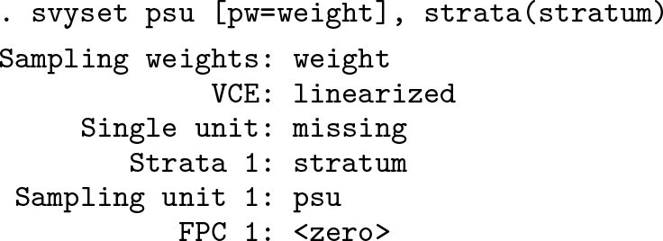
MPIs are frequently estimated using household survey data. To account for their complex survey design, it is convenient to rely on Stata’s suite of survey data commands; see [SVY] svy and [SVY] svy estimation. For the present example, first use svyset to specify the primary sampling unit, the strata, and the sampling weight for each observation; see [SVY] svyset for details.
For real-world data, the documentation of the respective dataset provides the relevant information. Next we specify indicators similar to the global MPI, which are organized in three dimensions (health, education, and living standards). We use mpitb set to assign indicators to dimensions and to provide names both for dimensions (hl, ed, ls) and for the entire specification (trial01).

Now assume the task is to estimate for the indicator selection trial01 all aggregate (M
0, H, and A) and indicator-specific measures (hd
, hd
(k), and absolute and percentage contributions). Further, let the preferred weighting scheme be the equal-nested one— that is, equal weights for all dimensions and equal indicator weights within dimensions— and let k = 20%, 33%, and 50% be of particular interest. Finally, we wish to obtain disaggregations by subnational regions and by area (that is, urban versus rural) and to account for the complex survey design. Hence, we issue mpitb est as follows:


mpitb est reports progress and results along three tabs. The first tab summarizes the underlying specification including the indicators, dimensions, and weights. The second tab shows the progress during the estimation procedures and details the numbers of so-far-accumulated estimates. The final tab provides a summary of the produced result frames or files, including the number of estimates, the type of measures estimated, and the respective level of analysis.
In the command above, we instructed mpitb est to store all results into a frame (see [D] frames) by using the lframe() option. All produced result files or frames follow a specific structure, which we now briefly explore.
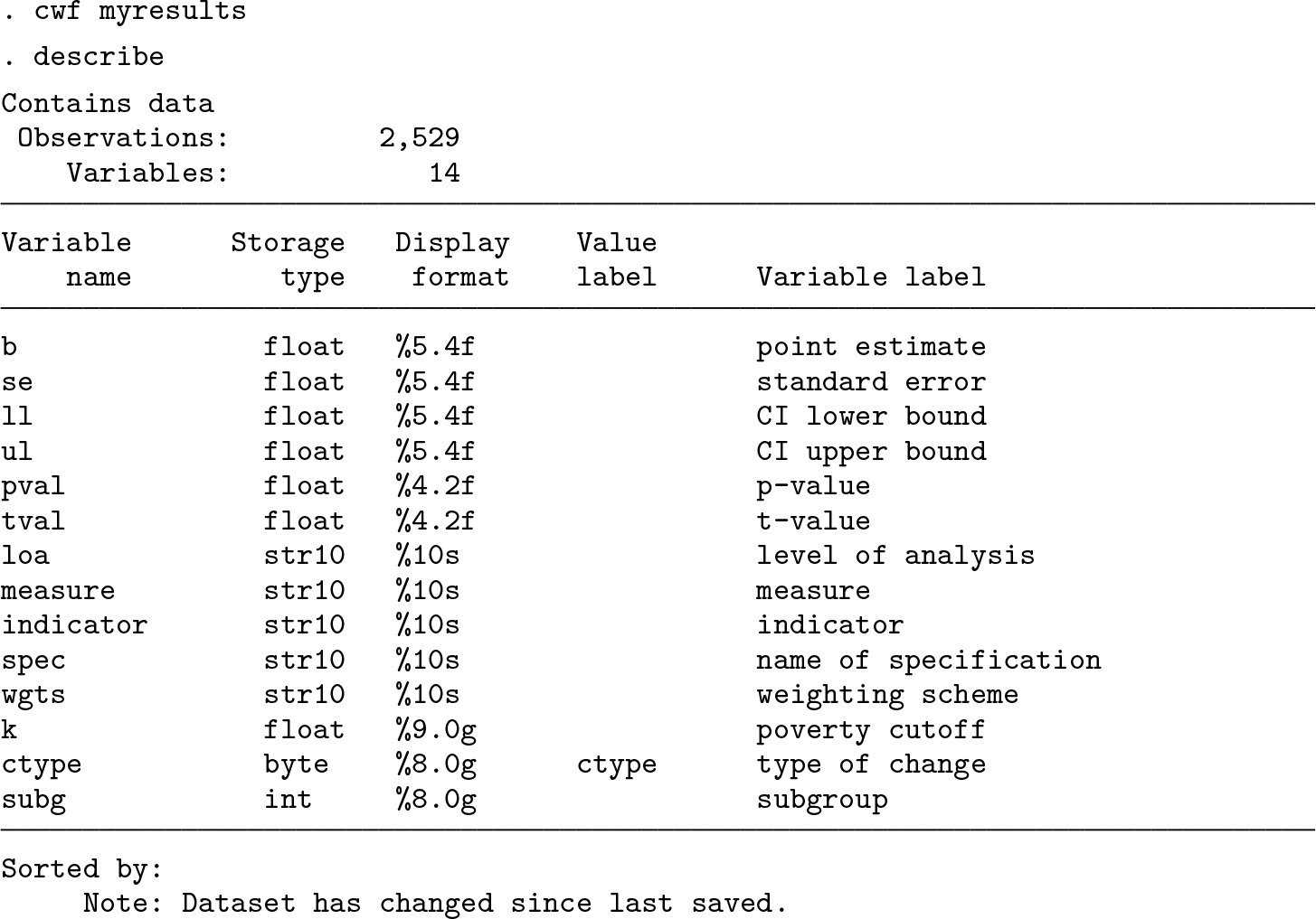
The key feature of this structure is that each observation represents an estimate. The core of each estimate includes the point estimate and its standard error (variables b and se), and the remaining meta variables specify the content for each estimate. See Suppa (2022) for a further discussion and Suppa and Kanagaratnam (2023) for details on the result files of the global MPI.
The result file may be conveniently explored using basic commands such as tab, list, or tabdisp. For instance, to see which measures are available for each level of analysis (loa), type
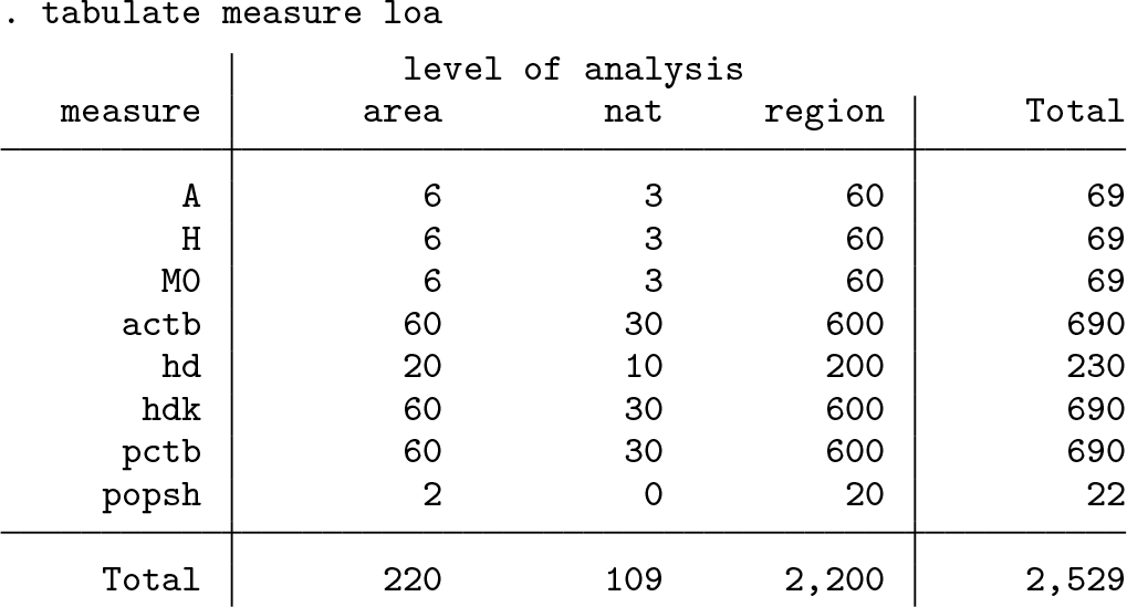
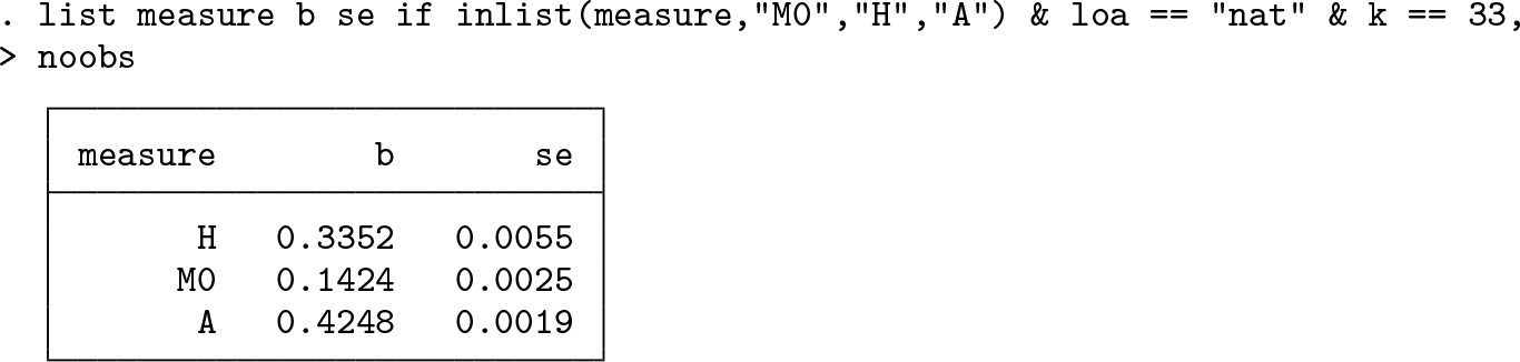
To directly inspect particular estimates and their standard errors, such as all aggregate measures at the national level for the preferred poverty cutoff, type
Often, it is convenient to have a variable for each level of analysis. These may be generated, for instance, as follows:

If we were interested in comparing censored and uncensored headcount ratios between urban and rural areas, a quick tabdisp provides first insights.
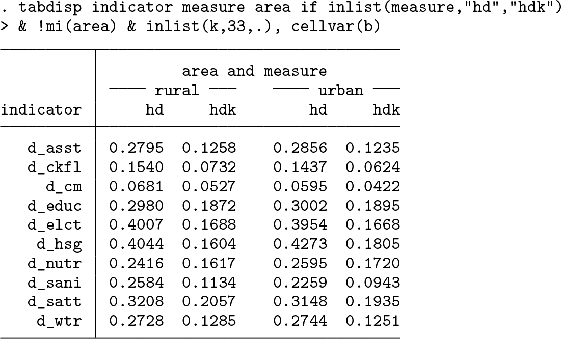
Note that tabdisp already allows construction of more-complex tables and even more through the revised table command; see [R] table. However, in this example, we will not cover proper labeling.
Example 2: Avoiding unnecessary estimations
In example 1, we stored the results in a frame. For examples 2 and 3, we will collect all estimates in files in a dedicated folder, which we call results, before we later combine them into a single file. This folder may be created using
. mkdir results
For multidimensional poverty measures, varying parameters may quickly make the numbers of estimates go through the roof. Having a clear sense of the priorities helps to guide any such analysis. Therefore, mpitb allows the user to reduce the number of estimates as needed.
For example, it is common to explore numbers for M
0, H, and A at the aggregate level for some 10 different values of the poverty cutoff over the entire domain of k, resulting in 30 estimates. Assuming an MPI with 10 deprivation indicators, the estimation of three indicator-specific measures for these values of k would add another 300 estimates at the aggregate level. For a country with 15 regions, another 1,500 estimates would have to be added on the subnational level.
To purposefully reduce the number of estimates, mpitb allows the user to specify different ranges of k for different layers of the analysis. By default, the range specified through option klist() is applied to all measures and levels of analysis. However, option indklist() allows specification of a separate range for the indicator-specific measures, whereas the over() option accepts suboption klist() to restrict the range of alternative parameters for disaggregations. Consider the following example, which only differs in the mpitb est command:

First, note that we now use the lsave() option to store the results immediately to disk. Moreover, describe tells us that the use of indklist() and the over() suboptions klist() and indklist() results in some 1,200 estimates instead of 8,600, thereby saving estimation time and simplifying the subsequent analysis.
1
Example 3: Adding alternative weights and indicator selections
So far, our results feature only a single weighting scheme. The toolbox allows setting alternative weights in different ways. To set custom dimensions-specific weights (with equal weights within dimensions), say, 50% for health and 25% for the other two, use the dimw(
numlist
) option as follows:

As seen above, one may similarly specify the alternative weighting schemes educ50 and livstd50.
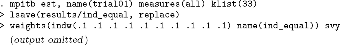
Sometimes, one may wish to assign custom indicator weights (for example, equal indicator weights). Option indw(
numlist
) allows this as follows:
Finally, to consider alternative indicator choices, such as without the deprivation indicator for electricity (d_elct), we first use mpitb set to set this specification, which we call trial02, and we then estimate the desired quantities.

This approach allows us to conveniently analyze the effects of i) dropping or adding single indicators, ii) alternative deprivation thresholds for one or more of the indicators, and iii) radically different indicator selections.
In this example, all results have been saved into a particular file each time mpitb est has been run. Often, it is convenient to assemble a single comprehensive result file. One way to achieve this is to append (see [D] append) all files as explicitly specified by a list. (For appending all files of a folder, see example 5.)

We now can explore our comprehensive results file as detailed above by using basic Stata commands such as tab or list.
Example 4: Several years for a single country
This section will illustrate how to estimate both levels and COT for all measures. Doing so requires repeated surveys for the same country, that is, at least repeated crosssectional data. A convenient way to organize such data is to have an identifier for each survey round and to append the microdatasets. In the sample data syn_cdta.dta, the time variable t may be 1 or 2. As before, we first load and svyset the data before we specify our preferred indicators:

If we were just interested in the estimation of the levels for the above specified measures in both years, we could simply add the tvar(t)option to the above mpitb est commands. The toolbox, however, also offers direct estimation of COT. The following command, for example, estimates not only the levels but also the COT for all specified measures, parameters, and levels of analysis.

Note again that this command stores frames and not files. Moreover, a dedicated frame for change estimates must be specified because required data structure for saving change estimates somewhat differs. More specifically, a change estimate is characterized by two points of time (a beginning and an end point), contains an absolute or relative change, and may be annualized (see also Suppa [2022] on this).
2
The required information on the duration of the period of observation is obtained from the option cotyear().
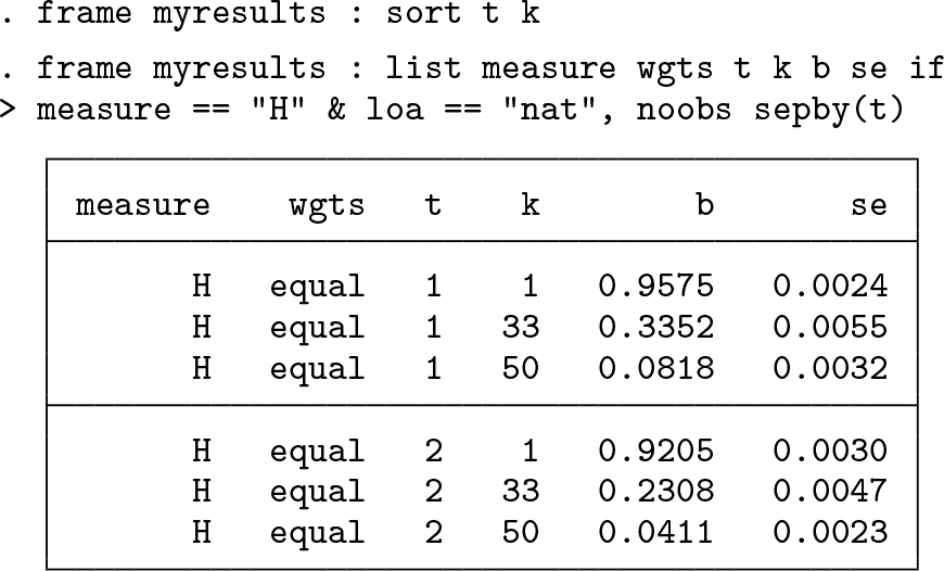
The level estimates are now stored in the frame myresults and may be conveniently inspected using list. To see, for instance, aggregate estimates of the headcount ratio for all k and t, proceed as follows:
The frame containing the results for COT may be explored in a similar fashion.

Example 5: A single year for several countries
A cross-country analysis may benefit even more from a careful folder structure. All cleaned microdatasets to be used in the estimation process are assumed to be stored in a dedicated folder that contains nothing else. The present example features three countries, and their datasets are stored in the folder cdta. Moreover, all outputs shall be stored in the results folder.

The first step is to compile the reference sheet, which will contain survey-constant information, such as the survey name (for example, “DHS”), the year (for example, “2015–2016”), and the names of subnational regions. The reference sheet may be used i) to control estimation and other production routines efficiently, ii) for easily merging external data, and iii) to reduce the amount of information that estimates are passed through the estimation routine. For more information on the reference sheet and its role in the global MPI workflow, see Suppa (2022).
The tool mpitb refsh first extracts the relevant information from each microdataset and then compiles this information into a single .dta file. mpitb refsh expects the path where the microdata are located and an ID to distinguish different countries. By default, the id(
name
) option expects the name of a variable but, if option char(
clist
) is set, also accepts the name of a data characteristic. Data characteristics are more efficient to store information that is constant for all observations in a given dataset; see [P] char for more details on data characteristics. The datasets of this example carry a data characteristic named ccty, which contains the ISO country code. Additionally, these datasets also feature data characteristics such as survey and year.

If issued without the sid() option, mpitb refsh would simply create a file with one observation per country.
By default, mpitb refsh reports region codes (region) and names (region_name) but also stores the filename (fname) and timestamps of the microdataset. Because survey datasets of some countries may not allow disaggregation by regions, mpitb refsh creates a single entry for countries for which the region variable only contains missing values. Note, however, that this variable has to exist in the microdataset.
It is convenient to have the reference sheet in a frame immediately at hand.

To perform an estimation across countries, first select the countries from the reference sheet by using mpitb ctyselect, which only expects the name of the variable containing the country codes. By default, mpitb ctyselect returns all available countries, but one may choose specific subsets using manually specified country codes, world regions, or regular expressions.
The following loop iterates over all the selected countries, first loading the microdata according to the filename in the reference sheet, then svysetting the data, then specifying the indicators of the MPI, and finally estimating as desired.

In the cross-country context, it is convenient to store results country-wise in files, by using the lsave() option. Moreover, the addmeta(
metalist
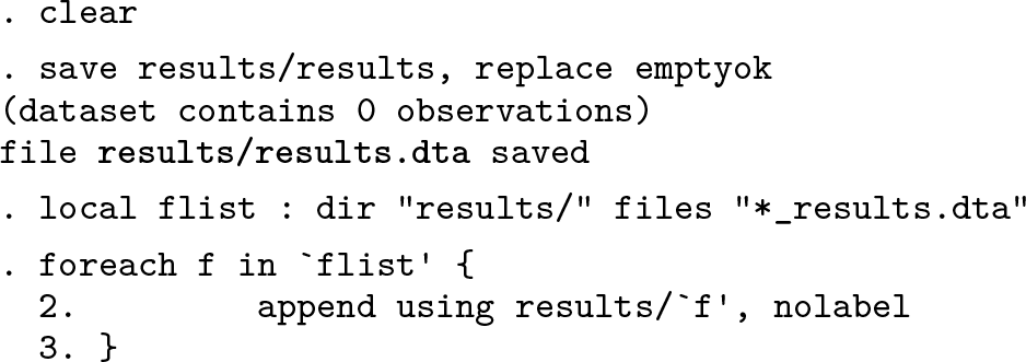
) option of mpitb est allows storage of the country code for each estimate as a meta variable (ccty) into the results file. To subsequently combine the country-specific files into a single result file, one may simply append all files stored in a single folder and potentially satisfy a particular filename pattern, as illustrated below.
Finally, one may add region names as provided by the reference sheet to the results file as follows:

Depending on the scale and the specific features of a particular project, it may be preferable to have both a results_raw.dta that contains only the appended data and a separate, more polished results.dta that additionally contains all the labeling as needed for the analysis or deliverable production.
Having a comprehensive cross-country results file allows the user to easily explore a wealth of data. For example, how do all three countries perform in key measures for the preferred parameterization?

Drawing on the labeling information collected by mpitb refsh also provides more informative analyses of subnational regions.

5 Conclusions
mpitb seeks to facilitate the work of both academics and practitioners of multidimensional poverty measurement. Because the toolbox has been developed in the context of the global MPI, it is also tailored to its needs, whether in terms of the underlying data, the quantities produced out of the box, or the related forms of analysis. Multidimensional poverty measurement and analysis is, however, an active field of research, where new measures, analyses, and other methodological innovations are still proposed and discussed. mpitb may already be useful for such endeavors and take some load off of researchers working these topics.
The very nature of mpitb as a toolbox seeks to allow for further features, novel analyses, and additional tools being added in the future. One natural extension is to implement the estimation of other poverty indices proposed in the literature (for example, Bourguignon and Chakravarty [2003] and Bossert, Chakravarty, and D’Ambrosio [2013], among many others); see Alkire et al. (2015) and Aaberge and Brandolini (2015) for a discussion of some of them. Likewise, adding support for novel complementary measures within the AF framework, for example, for the analysis of inequality among the poor (Alkire and Foster 2019) seems natural. Extensions along these lines may be implemented directly into mpitb est.
Other types of analyses, however, may require one or more tools on their own, such as a panel-data-based analysis within the AF framework (for example, Alkire et al. [2017a], Suppa [2018]). Standalone tools may also be needed for the analysis of pairwise robust comparisons, which examines country orderings in terms of their poverty indices (Alkire and Santos 2014; Alkire et al. 2022a), or the recently proposed modeling framework for computing projections of multidimensional poverty (Alkire et al. Forthcoming).
Aside from the implementation of genuine methodological innovations, one may also consider convenience tools, which, for instance, help to compare different measures using specific tabulations or visualizations during the trial stage. Future developments, however, depend on many factors, including user needs, further progress in research, and available resources.
