Sage Journals: Discover world-class research

Abstract

Interaction analyses are useful tools to examine complex socioeconomic outcomes in which the effect of one variable depends on the presence or values of another variable. Interaction effects capture simultaneous changes in two (or more) covariates, and their computation is especially challenging in nonlinear models. For such models, a statistically significant interaction-term coefficient does not necessarily indicate significant interactive effects. For analyses in which the interaction effect cannot be inferred from the model estimates, I introduce ginteff, a new command that automatically computes two- and three-way interaction effects. The command accommodates a large suite of estimation models and allows researchers to use either the partial derivative or the first difference to model the effect of the interacted variables.

Keywords

st0711 ginteff ginteffplot average interaction effect individual-level interaction effects two-way interactions three-way interactions

1 Introduction

Interaction analyses are used to examine complex socioeconomic outcomes in which the effect of one variable depends on the presence or values of another variable.¹ For example, to assess whether the 2008 financial crisis had a more pronounced effect on minorities, in a regression analysis, we would interact (that is, multiply) the indicator of minority status with that of the before- and after-2008 periods. In linear models, the coefficient on the interaction term can be used to infer whether the effect of the treatment variable is statistically different at alternative values of the moderating variable. For instance, if the interaction coefficient were to reach the conventional levels of statistical significance, we would conclude that the 2008 crisis had a statistically different effect on majority and minority groups. In nonlinear models, however, the coefficient on the interaction term does not tell us the direction, magnitude, or significance of the interaction effect (Ai and Norton 2003). For analyses in which the interaction effect cannot be inferred from the model estimates, I introduce ginteff, a new command that automatically computes two- and three-way interaction effects. The command accommodates a large suite of estimation models and allows researchers to use either the partial derivative or the first difference to model the effect of the interacted variables.

2 What is an effect and how do we calculate it?

Broadly speaking, the interaction effect is the change in the effect of a given variable as another variable also changes. Before considering two simultaneous changes, I briefly review what an unconditional effect is and how it is computed. Let us say our dependent variable y depends on the independent variable of interest, x, and a vector of other covariates plus the constant term, X. Conditional on the independent variables, the predicted value of y is

Pr (y | x, X) = F (β_{x} x + β X)

where F (·) is the (possibly nonlinear) link function of model predictors.² The effect of x on y is the change in Pr(y) attributable to a change in x. There are two general approaches to computing the effect of x, which I denote by Δ(x). One alternative is to calculate the first difference, which is the change in Pr(y) associated with an n-unit increase in x (frequently a one-unit increase), Δ(x) = {Pr(y|x + n) − Pr(y|x)}. This is the default approach for factor variables, in which case the effect is the discrete change from the base level. For example, if x is a dummy variable, the discrete difference is Δ(x) = Pr(y|x = 1) − Pr(y|x = 0).

For continuous variables, researchers can alternatively compute the instantaneous rate of change, which is the partial derivative with respect to x, Δ(x) = {∂Pr(y)}/(∂x). This estimate can then be used to calculate the impact on y of a very small increase, say, 0.001, in x.³ In this case, Pr(y) would increase by about 0.001 × Δ(x). In practice, however, many analysts extrapolate and interpret the value of Δ(x) as representing the change in y associated with a one-unit increase in x. In many (but not all) instances, this is a good approximation. In nonlinear models, there is no guarantee that a one-unit increase in x would lead to a change in y of 1 × Δ(x). In fact, substantive deviations are likely when x is measured in large units (Williams 2012, 2021).

Turning to interactions, let us say we have a multiplicative model where two independent variables, x ₁ and x ₂, are interacted. In this case, the predicted value of y is

Pr (y | x_{1}, x_{2}, X) = F (β_{1} x_{1} + β_{2} x_{2} + β_{12} x_{1} x_{2} + β X)

One can use either the partial derivative or the first difference to compute the simultaneous changes in x ₁ and x ₂. Specifically, the interaction effect can be computed as the cross-partial derivative with respect to both variables, {∂ ²Pr(y)}/(∂x ₁∂x ₂), or as the discrete difference between two first differences, {Pr(y|x ₁ + n ₁; x ₂ + n ₂) − Pr(y|x ₁; x ₂ + n ₂)} − {Pr(y|x ₁ + n ₁; x ₂) − Pr(y|x ₁; x ₂)}. Technically, they are both valid approaches. From a purely practical perspective, the first-difference approach has several advantages. First, it does not require complex math, because we need to compute predicted probabilities only for alternative values of x ₁ and x ₂. By contrast, taking the cross-partial derivative is a challenging task even for relatively simple likelihood functions and may be intractable for complex ones. Second, it is easier to explain what the interaction effect represents in substantive terms when using clearly defined increments (for example, a one-unit increase). By contrast, partial effects reference an undefined “very small” amount.⁴

3 The ginteff command

3.1 Description

ginteff computes the average and individual-level interaction effects for two- and three- way interactions. The effect of the interacted variables can be computed via either the partial derivative or the first difference.

3.2 Syntax

3.3 Options

Short descriptions of the ginteff options are presented in table 1. For the extended descriptions, see The ginteff User’s Manual.

Table 1.

The ginteff options

	effect_computation	Description
*	dydxs( dxspec )	specify the interacted variables for which to compute the effect via partial derivative
	fd( fdspec )	shorthand for firstdiff()
*	firstdiff( fdspec )	specify the interacted variables for which to compute the effect via first difference
* One of dydxs() or firstdiff() is required. A minimum of two and a maximum of three variables must be specified in dydxs() or firstdiff().
	options	Description
	atdxs( atdxspec )	fix the interacted variables in dydxs() to specified values
	nunit(( # ) varlist )	specify the unit increase for each variable in firstdiff()
	obseff( stub )	create new variables with the interaction effect for each observation
	at( atspec )	compute the interaction effect at specified values of covariates
	intequation( eqno )	identify the interaction equation; default is intequation(#1)
	level( # )	set confidence level; default is level(95)
	many	report more than 100 results; maximum is 1,000
	nolegend	suppress output legend
	noweights	ignore weights specified in estimation
	post	post interaction effects and their variance–covariance estimate as estimation results
	predict( pred_opt )	compute the interaction effect for predict, pred_opt
	vce( vcetype )	specify how the variance–covariance estimate and standard errors are calculated; default is vce(delta)

3.4 Stored results

ginteff stores the following in r():

4 The ginteffplot command

4.1 Description

ginteffplot graphs the results of the immediately preceding ginteff command.

4.2 Syntax

ginteffplot [, options]

4.3 Options

Short descriptions of the ginteffplot options are presented in table 2. For the extended descriptions, see The ginteffplot User’s Manual.

Table 2.

The ginteffplot options

options	Description
Main
aiepoint([# _{clockposstyle}] ["text for label "] [ , marker_label_options marker_options ])	customize marker for the point estimate of the average interaction effect
aierange([line_options] [msize(markersizestyle )] )	customize the range plot of the average interaction effect using capped spikes
Obseff [(obseff_options )]	plot observation-level interaction effects
output( # )	identify a specific ginteff output to be graphed; default is output(1)
save(newfile .suffix [, export_options] )	export current graph
xcommon([numlist] [*] )	give x-axes common scale
zeroline [(line_options )]	add a vertical line at the 0 value
x and y axes
xtitle( axis_title )	customize x-axis title
ytitle( axis_title )	specify y-axis title
xlabel( rule_or_values )	customize ticks and labels for x axis
ylabel( rule_or_values )	specify ticks and labels for y axis
xscale( axis_suboptions )	customize how x axis looks
yscale( axis_suboptions )	specify how y axis looks
Plot and graph areas
aspectratio(# [, pos_option] )	plot region aspect ratio
graphregion( suboptions )	customize attributes of graph region
plotregion( suboptions )	customize attributes of plot region
scheme( schemename )	customize the graphics scheme
xsize( # )	change width of graph
ysize( # )	change height of graph
Titles, legend, and notes
legend( [contents] [location] )	standard legend, contents, and location
note( tinfo )	note about graph
title( tinfo )	overall title
subtitle( tinfo )	subtitle of the graph

5 What is new or different with ginteff?

In this section, I first compare and contrast ginteff with existing community-contributed commands and then with Stata’s official commands.

5.1 Comparing ginteff with community-contributed commands

There are two community-contributed commands for calculating interaction effects, that is, inteff and inteff3, for two- and three-way interactions, respectively (Cornelißen and Sonderhof 2009; Norton, Wang, and Ai 2004). These commands have significantly increased our understanding of interaction models and helped analysts correctly compute interaction effects. Yet they accommodate only logit and probit models, and if the interaction involves factor variables, they must be dummy variables. In fact, inteff3 can handle solely binary variables and cannot be used with continuous variables. inteff can compute the effect of a continuous-by-continuous interaction via the cross-partial derivative, but alternative modeling options are excluded (for example, the first difference). Another restriction is that numeric variables cannot have higher-order terms (for example, squared terms).

ginteff has none of these limitations. Specifically, ginteff extends the computation of interaction effects to cases in which factor variables have more than two categories. It also allows researchers to choose whether to compute the effect of the interacted variables via the partial derivative or the first difference. Additionally, ginteff accepts weights (thus accommodating survey analyses), and the interacted variables can have higher-order terms. Last, ginteff can be used after a wide range of estimation models because it accommodates most models after which margins can be used. This includes regression models for panel data (for example, xtreg, xtlogit); models for censored or truncated data (for example, truncreg, tobit); and multiequation models (for example, biprobit, sureg). It can also be used after models with a polychotomous dependent variable, and the outcomes may be either ordered or not (for example, ordered logit, multinomial logit). In sum, ginteff is more general than its predecessors.

ginteff also features a simplified syntax and a larger set of options. For instance, users need not provide the names of the interacted variables in a particular sequence.⁵ Besides offering increased flexibility, many elective options have the same syntax as the homonym options of margins (for example, at(), level(), noweights, post, predict()). Because Stata users are already familiar with these options, this should facilitate the adoption of the new command.

This said, ginteff comes with one notable restriction. It can estimate interaction effects between continuous variables via the cross-partial derivative only for logistic, logit, and probit models. Even when considering the restricted set of models, computing three-way interaction effects for continuous variables is a novel feature that inteff3 does not possess. This limitation, though, does not concern interactions involving factor variables or analyses in which the effect is computed via the first-difference approach. For clarity, there are no model restrictions when the interaction is between 1) one factor and one continuous variable, 2) two factor variables, 3) two factor variables and one continuous variable, 4) three factor variables, and, if one is using the first-difference approach, 5) two continuous variables, 6) one factor variable and two continuous variables, and 7) three continuous variables.

Technicalities aside, the substantive difference between ginteff and its predecessors is that the former computes the average interaction effect, whereas the latter compute individual effects for each case in the data.⁶ The decision to compute the average or case-level effects boils down to one’s view about how to best report nonconstant effects. This goes beyond interaction effects because it concerns marginal effects in nonlinear models more generally. In nonlinear models, even the unconditional effect of a variable differs from one observation to the next because the magnitude of the effect is conditional on the values of other covariates, which are case specific. Thus, there is no one single effect.

Each approach comes with its own advantages and disadvantages. The case-level approach entails computing the interaction effect separately for each individual observation. Because it reveals the heterogeneity of individual effects, this approach can prevent gross generalizations. The alternative approach is to aggregate the individual effects and report the average. The advantage is that we can make inferences about a variable’s effect in the population or specific subgroups. This approach is particularly useful when individual cases are anonymous and do not carry special meaning. For example, when examining the effect of an initiative to increase voter turnout, it is the average response that is of immediate interest. In fact, a report that focuses on individuals’ idiosyncratic responses may be of little practical relevance to policymakers.

It is beyond the scope of this article to compare the two approaches. In practice, their usefulness depends on the research question and type of data (for example, the voting record of the nine U.S. Supreme Court justices or a large population survey). Importantly, ginteff users can still compute the interaction effect for each observation via option obseff(). Because it can estimate both the average and the individual-level effects, ginteff offers researchers more options to analyze the data.

5.2 Comparing ginteff with Stata’s official commands

Most ginteff results can be reproduced via margins because, behind the scenes, it is this Stata command that does the heavy lifting when computing interaction effects. However, there are some notable exceptions. For example, margins cannot automatically calculate two- or three-way interaction effects between continuous variables via the partial derivative. Because dydx() can take just the first derivative, it cannot be used for second- and third-order cross-partial derivatives. To calculate two- and three-way interaction effects, the user must write the correct vector notation formula in option expression(). Similarly, one cannot directly compute interaction effects via the firstdifference approach. For instance, to compute a three-way effect, one needs to first correctly specify eight distinct at() options. These represent all combinations between the initial value and the counterfactual increase in the interacted variables. Then, the user must correctly subtract the respective predictive margins with the exact sequence varying based on the order in which the at() options were introduced. This second step also requires the use of a different command, nlcom. These intermediary steps can be taxing and error prone.⁷

ginteff also has extra features that provide additional options and checks. For instance, one cannot simultaneously calculate the average and individual-level interaction effects using margins.⁸ This task is straightforward with ginteff because option obseff() automatically computes the interaction effect for each observation. Furthermore, ginteff also checks that the specified variables are actually interacted and there are no missing terms. For example, the analyst is notified if only two terms of a threeway interaction are listed.

Ultimately, having a specialized command to compute interaction effects minimizes mistakes. margins is a general command that can compute many quantities of interest, whereas ginteff is a one-stop command for most interaction effect calculations. While being versatile is an appealing feature of margins, it can also overwhelm users. For instance, there is more than one alternative to compute a given quantity of interest via margins. Specifically, some show how to compute interaction effects for factor variables using the contrast option (for example, Wiggins [2004]), while others show how to do so using pwcompare (for example, Pinzon [2016]). Combining the reference manuals for 1) margins, 2) margins, contrast, and 3) margins, pwcompare amounts to over 80 pages of dense information detailing dozens of options.

6 Interpreting interaction effects

Before showing how ginteff can be used to compute interaction effects, I briefly review how to interpret them. Let us assume we have an interaction between two dummy variables, x ₁ and x ₂, and the predicted value of y is a function of the interacted variables as well as other covariates,

Pr (y | x_{1}, x_{2}, X) = F (β_{1} x_{1} + β_{2} x_{2} + β_{12} x_{1} x_{2} + β X)

For dummy variables, the marginal effect is the first difference, that is, the change in Pr(y) in the presence and absence of that variable. In practice, this means calculating F(β ₁x ₁ + β ₂x ₂ + β ₁₂x ₁x ₂ + β X) when the variable of interest is set to 0 and 1 and then subtracting the former from the latter. The interaction effect, in turn, is the discrete double difference with respect to both x ₁ and x ₂ or the difference between two first differences (Norton, Wang, and Ai 2004, 157):

\begin{array}{l} \frac{Δ^{2} \Pr (y)}{Δ x_{1} Δ x_{2}} = \frac{Δ \frac{Δ \Pr (y)}{Δ x_{1}}}{Δ x_{2}} \\ = \frac{Δ \frac{Δ F (β_{1} x_{1} + β_{2} x_{2} + β_{12} x_{1} x_{2} + β X)}{Δ x_{1}}}{Δ x_{2}} \\ = \frac{Δ {F (β_{1} \times 1 + β_{2} x_{2} + β_{12} \times 1 \times x_{2} + β X) - F (β_{1} \times 0 + β_{2} x_{2} + β_{12} \times 0 \times x_{2} + β X)}}{Δ x_{2}} \\ = \frac{Δ {F (β_{1} + β_{2} x_{2} + β_{12} x_{2} + β X) - F (β_{2} x_{2} + β X)}}{Δ x_{2}} \\ = {F (β_{1} + β_{2} \times 1 + β_{12} \times 1 + β X) - F (β_{1} + β_{2} \times 0 + β_{12} \times 0 + β X)} \\ - {F (β_{2} \times 1 + β X) - F (β_{2} \times 0 + β X)} \\ = F (β_{1} + β_{2} + β_{12} + β X) - F (β_{1} + β X) - F (β_{2} + β X) + F (β X) (1) \end{array}

What does the interaction effect, {Δ²Pr(y)}/(Δx ₁Δx ₂), mean in substantive terms? To answer this question, we need to understand what each of the four elements on the right-hand side of (1) represents. To make the interpretation more concrete, let us assume we want to assess the effect of gender and race on health. Among other determinants, one’s health is a function of both gender (0 = male, 1 = female) and race (0 = majority, 1 = minority), and the two condition each other’s effect. The dependent variable is a dummy indicator of health (0 = poor and 1 = good). For models with a binary dependent variable, y ∈ {0, 1}, where the probability space is bounded between 0 and 1, a popular nonlinear function is the cumulative standard logistic distribution, Λ(·), which leads to the logit model. Specifically, this distribution function is Λ(β X) = (e ^β ^X )/(1 + e ^β ^X ) = 1/(1 + e^−β ^X ) = Pr(y = 1), where Pr(y = 1) is the probability of the event occurring (Clark and Golder 2023, 297).

For our example, we can write the probability of being in good health as

\Pr (h = 1) = Λ (β_{f} f + β_{r} r + β_{f r} f r + β X) = \frac{1}{1 + e^{- (β_{f} f + β_{r} r + β_{f r} f r + β X)}}

where h is the health indicator, f stands for female, and r stands for race. When we replace y with h, x ₁ with f, x ₂ with r, and F(·) with Λ(·), the four right-hand-side elements of (1) become

\begin{array}{l} \frac{Δ^{2} Λ (h)}{Δ f Δ r} = Λ (β_{f} + β_{r} + β_{f r} + β X) - Λ (β_{f} + β X) - Λ (β_{r} + β X) + Λ (β X) \\ = \frac{1}{1 + e^{- (β_{f} + β_{r} + β_{f r} + β X)}} {\Pr (h = 1 ∣ f = 1, r = 1)} (2) \\ - \frac{1}{1 + e^{- (β_{f} + β X)}} {\Pr (h = 1 ∣ f = 1, r = 0)} (3) \\ - \frac{1}{1 + e^{- (β_{r} + β X)}} {\Pr (h = 1 ∣ f = 0, r = 1)} (4) \\ + \frac{1}{1 + e^{- (β X)}} {\Pr (h = 1 ∣ f = 0, r = 0)} (5) \end{array}

To help with the interpretation, I note in curly braces what each element means in terms of predicted probabilities. For example, (2) captures the probability of being in good health (h = 1) for a woman (f = 1) who is a member of a racial minority (r = 1). Similarly, (3) captures the probability of being in good health for a woman who is a member of the majority group (r = 0), and so on. For convenience, I will reference the respective probabilities by the corresponding equation number (that is, Pr_{Eq. (2)}, Pr_{Eq. (3)}, Pr_{Eq. (4)}, and Pr_{Eq. (5)}).

Without altering the result, we can rearrange the four probabilities as the difference between two distinct differences: (Pr_{Eq. (2)} − Pr_{Eq. (4)}) − (Pr_{Eq. (3)} − Pr_{Eq. (5)}). The first parenthetical statement, (Pr_{Eq. (2)} − Pr_{Eq. (4)}), captures the difference in the probability of being healthy between a minority female and a minority male. Put differently, this is the effect of gender on health for racial minorities. The second parenthetical statement, (Pr_{Eq. (3)} − Pr_{Eq. (5)}), captures the difference in the probability of being healthy between a woman and a man from the majority group. Thus, this is the effect of gender on health for the racial majority. Finally, the difference in the effect of gender between the minority and majority groups is the interaction effect. Substantively, it captures the relative strength of the two gender effects. For instance, a positive value on the interaction effect would indicate that the effect of gender on well-being is more pronounced for minorities than for the majority group.⁹

The interpretation of the interaction effect would be similar if gender were interacted with a continuous variable such as age. In this case, the interaction effect would capture the relative strength of the two gender effects attributable to an n-unit increase in age. More specifically, we would compare the effect of gender between the current group of respondents and a counterfactual group where respondents were one year older (assuming the standard one-unit increase in x).

Last, we could also have an interaction between two continuous variables, say, age and income (measured in thousands of dollars). In this example, the interaction effect would capture the effect on health of a one-unit increase in income (that is, $1,000) attributable to a one-unit change in respondents’ age. More specifically, we would compare the effect of increasing the respondents’ income by $1,000 with the effect of the same income bump for a counterfactual group where respondents were one year older.¹⁰

7 Computing interaction effects with ginteff

I illustrate the capabilities of the ginteff command using data from the Second National Health and Nutrition Examination Survey, available from the StataCorp website. The dependent variable (DV) is health, which codes the respondents’ well-being on a five-point scale (that is, poor, fair, average, good, and excellent). The independent variables are age, female, and race; age is numeric, whereas female and race are factors. female is coded 0 for males and 1 for females. race is a three-category variable in which 1 = white, 2 = black, and 3 = other. In the upcoming examples, female and race are the interacted variables, and age is used as a control.¹¹ To keep things concise, I frame the discussion around the effect of gender on health. But the estimated effects also apply to race because cross-partial derivatives are symmetric. Last, these exercises are for illustration purposes only. In particular, I do not test a specific hypothesis or include all relevant predictors.

7.1 A binomial logit example

For this exercise, I use a dichotomous indicator of health coded 1 if the respondent’s health is above average and 0 otherwise. Specifically, the dummy DV is obtained by collapsing the poor, fair, and average levels into one category and the good and excellent levels into another category.

After getting the data, I first fit an additive logit model with no interactions as a reference point. The coefficient on female is negative and statistically significant, which means that, keeping everything else constant, females are less likely to be in good health than men. Because logistic regression is a nonlinear model, the coefficient estimate is not the same as the average marginal effect. Setting race and age at their observed values, I compute the effect of gender on health using margins. The generate(obs_noint) option calculates the predicted probability, separately for males and females, for each case in the data (the _noint suffix is shorthand for “no interaction”). The results are saved in two variables called obs_noint1 and obs_noint2. The difference between these variables is the individual-level marginal effect of gender. The level(90) option simply instructs margins to report the 90% confidence interval (CI) instead of the default, the 95% CI.

I plot the margins results in figure 1, where the average marginal effect of gender is indicated by the solid square mark and the horizontal line is the 90% CI. On average, the probability of being healthy is 0.031 [−0.046, −0.016] percentage points lower for females. This effect is statistically significant because the 90% CI does not contain zero. Thus, compared with men, women are significantly less likely to be in good health. To judge whether the average value represents a good measure of central tendency, I also plot the individual marginal effects for all cases in the data. These are indicated by the string of dots below the average effect. Because overlapping values may obscure the distribution of individual effects, the median is superimposed. While the average and median values are very similar, there is still variation among individual responses. This variation is not due to interactions directly modeled (there are none) but rather to the fact that, in nonlinear analyses, even unconditional effects depend on the values of all model covariates.¹²

Figure 1.

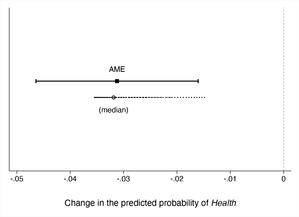
The marginal effect of gender on health (dichotomous indicator)

Next I fit a new model where female and race are interacted. To compute the average interaction effect, I then issue the ginteff command. The obseff(obs_l2w) option instructs ginteff to also compute the interaction effect for each observation (the _l2w suffix is shorthand for “logit model with a two-way interaction”). These results are saved in two variables, obs_l2w1 and obs_l2w2, one for each contrast of race (that is, change from the base level).

Before moving to interpreting and presenting the results, let us examine the ginteff output to understand what information each line conveys. The first line of the output (that is, the left-aligned text at the top) spells out that interaction effects are the substantive quantities of interest computed by the ginteff command. The second line clarifies that the main statistic reported in the results table is the average interaction effect. The third line specifies how the standard error of the average interaction effect is calculated (here the delta method).

The next lines introduce the interacted variables, x ₁ and x ₂. (For three-way interactions, there will also be an x ₃ variable.) For each individual variable, the associated line lists its full name and details how its effect, Δ(x _∗), is computed. Let us consider x ₂, which corresponds to variable race. The first thing to note is that the label of the effect, Δ(i.x2), includes i., conveying that the respective variable is a factor. After the colon, the Δ(·) notation is explained. In this case, it refers to the partial derivative of Pr(y) with respect to x ₂ (abbreviated to dy/dx); w.r.t. is shorthand for “with respect to.” Because the variable at hand is a factor, the partial derivative is the discrete change from the base level. After the semicolon, the x2 label is elaborated upon. The additional details comprise the base level (here b1, meaning race = 1) and the list of factor levels for which the discrete change is to be calculated (enumerated in the i() parentheses). In this example, this is all other levels of race, {2, 3}, which is the default. But one can specify a single level or, for factor variables with many levels, a subset of levels (see example 2 from The ginteff User’s Manual for a concrete example). Finally, the full name of the variable is displayed at the end.¹³

The next line of the output notes the number of observations used in the calculation. The last part of the output header spells out the expression of the response for which the effect is calculated. For our example, this is the probability of a positive outcome, Pr(health_2l = 1), which is the default after logistic regression. But we could have requested the linear prediction instead via the predict(xb) option or some other specified prediction. Knowing the type of the response is important because it informs the interpretation of the interaction effect. Because the response is the probability of a positive outcome in our case, the interaction effect can be interpreted as the change in the predicted probability of being in good health attributable to a change in both gender and race. Thus, the interpretation of the interaction effect depends on the outcome metric of the response, which is determined in part by the estimation model. For example, after linear regression, the interaction effect captures the change in the average value of y, but the change in the predicted number of events after a Poisson regression.¹⁴

When the analyst calculates the interaction effect for multiple at() scenarios, the legend showing the fixed values of covariates for each scenario will be displayed just above the table of results (see example 2 from The ginteff User’s Manual).

The results table shows the value of four estimates: the average interaction effect, its standard error, and the lower and upper limits of the associated CI. These are the table columns. Each row is associated with a distinct interaction effect, and the respective label clarifies the specific scenario. In our example, there are two outputs, one for each contrast of race. The first row output, labeled Δ(1.x1)#Δ(2.x2), is the interaction effect associated with a discrete change in x ₁ (female) from the base level to the factor level 1 and a discrete change in x ₂ (race) from the base level to the factor level 2. In practical terms, this means moving from males to females and from whites to blacks. The variables represented by x ₁ and x ₂, and their respective base levels, are indicated in the output header. The label of the second output, Δ(1.x1)#Δ(3.x2), indicates that the respective interaction effect is attributable to the same discrete change in female, but a change in race from the base level to the factor level 3 (racial minorities other than black).

In figure 2a, I graph the estimated average and individual interaction effects separately for both outcomes. Plotting the ginteff results is easily achieved using the companion ginteffplot command. For instance, figure 2a1 was generated simply by typing

. ginteffplot

The ginteffplot command automatically retrieves the point estimate of the average interaction effect (the solid square mark) and its upper and lower confidence limits (the horizontal capped spike). The significance level of the CI is set by the previous ginteff command. The name for the dependent variable used in the x-axis title (that is, Dummy health) is the label of health_2l, which I defined when creating this variable. The graph indicates that, on average, the negative effect of gender is statistically larger for blacks compared with whites (that is, the base category of race). Thus, women are generally less likely than men to have above-average health, and furthermore, black women fare worse than white women. The substantive difference is a decrease in the probability of being in good health of 0.056 [−0.102, −0.010] percentage points.

Figure 2.

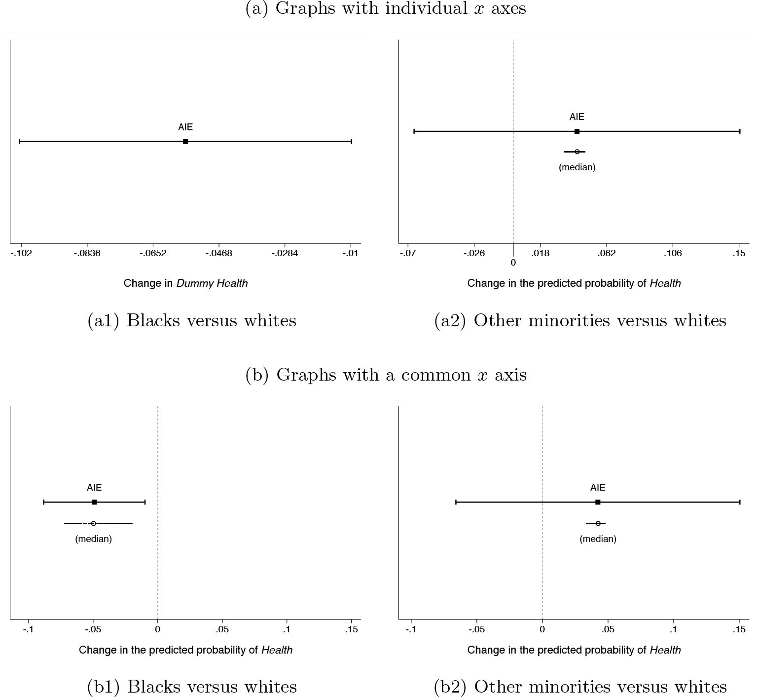
The interaction effect between gender and race on health (dichotomous indicator)

By contrast, women from racial groups other than black seem to fare better than white women. Specifically, the positive estimate in figure 2a2 indicates that the negative effect of gender on health is smaller for minority respondents. However, this effect is not statistically significant. Compared with figure 2a1, this graph has several extra features. First, the x title is more informative because it spells out what the outcome metric is, namely, predicted probability. Second, the plot displays a vertical line at the zero value to more easily judge whether the interaction effect is statistically significant. Third, it reports the full range of individual effects for all cases in the data with the median value superimposed. Because the individual effects are clustered and the median and mean values are very similar, the average represents a good measure of central tendency in this case. The command line to produce the enhanced figure 2a2 is

Option output(2) indicates that we want to plot the second row estimate from the results table.

By default, the ginteffplot command considers only the values for an individual output. This is fine when we estimate a single interaction effect or are mainly interested in assessing whether a given effect is statistically significant. However, if we want to evaluate one interaction effect in relation to another, we need to adjust the graphs so that they use the same scale. More specifically, all plots should have a common x axis. This can be achieved using the option xcommon()—where we can specify one other ginteff output, #; a subset of outputs, numlist; or all outputs, *—to be put on a common x-axis scale. I illustrate this option in figure 2b, which shows the same interaction effects from figure 2a but with plots that share the same x axis. The two graphs were produced by typing

Having the graphs on the same scale facilitates comparisons across outcomes and scenarios, but this should not be taken as a definitive significance of differences test. Specifically, when the CIs of two point estimates overlap, the estimates may or may not be different from one another (Goldstein and Healy 1995; Radean Forthcoming; Schenker and Gentleman 2001). Importantly, this is the case even if the point estimates have different signs and only one of them is statistically significant (Gelman and Stern 2006). This is the situation in our example because the two interaction effects are −0.056 [−0.102, −0.010] and 0.042 [−0.066, 0.151]. When the CIs overlap, the solution is to conduct a standard significance of differences test. For that, we need to first save the results, along with the estimated variance–covariance matrix in e(), by specifying option post. We can then pass these estimates to other commands (for example, nlcom) and conduct additional tests.

To illustrate this procedure, I reissue the previous ginteff command, using quietly to suppress the output. The main difference is that now the results are saved in e() because option post is specified. We can confirm this by listing the coefficient vector e(b). It is easy to see that these are the ginteff estimates, not the coefficients from the logit model. Last, I use nlcom to test whether the difference between the two interaction effects is statistically significant. Because the 90% CI of the difference in estimates contains 0, the respective effects are not statistically distinct at the 0.1 significance level. This is despite all conjectural evidence pointing to the contrary (that is, the compared estimates have opposite effect signs and different statistical significance status).

7.1.1 An ordered logit example

One of the advantages of ginteff over existing community-contributed commands is that it can accommodate models other than the binomial logit or probit. As an illustration, I next present an application concerning an ordered logit model. The data are the same as before, but now the DV is an ordinal variable, health_3l, with three levels, where 1 = poor, 2 = average, and 3 = excellent. Practically, I collapse the poor and fair levels into one category, keep the average category unchanged, and collapse the good and excellent levels into another category.

Let us consider the same two-way interaction between gender and race. Upon fitting the new model, I issue the ginteff command, which is identical to the one used after the simple logit (save the stub name in option obseff(obs_ol2w), with the new suffix being shorthand for “ordered logit model with a two-way interaction”). The first thing to note is that there are three times as many output results. Because now we have three distinct health outcomes, the interaction effect is computed separately for each of them. Second, ginteff automatically incorporates any auxiliary parameters into the calculations of interaction effects (here /cut1 and /cut2), removing the need for manual manipulation.

Figure 3 graphs the ginteff results by outcome and race. For easy comparison, all plots use a common x-axis range. Figure 3a1 outlines the difference between the conditional effect of gender for blacks and whites, 0.061 [0.020, 0.102]. The positive estimate means that black women are more likely to be in poor health than white women. When it comes to the average and excellent health outcomes, black women are less likely to be in good health (figures 3a2 and 3a3, respectively). All three interaction effects are statistically significant. The gender effect, however, has the opposite impact when we compare whites with other racial minorities. Specifically, women from minority groups other than black are less likely to be in poor or average health compared with white women and more likely to have excellent health. However, none of these effects are statistically significant (see figure 3b).

Figure 3.

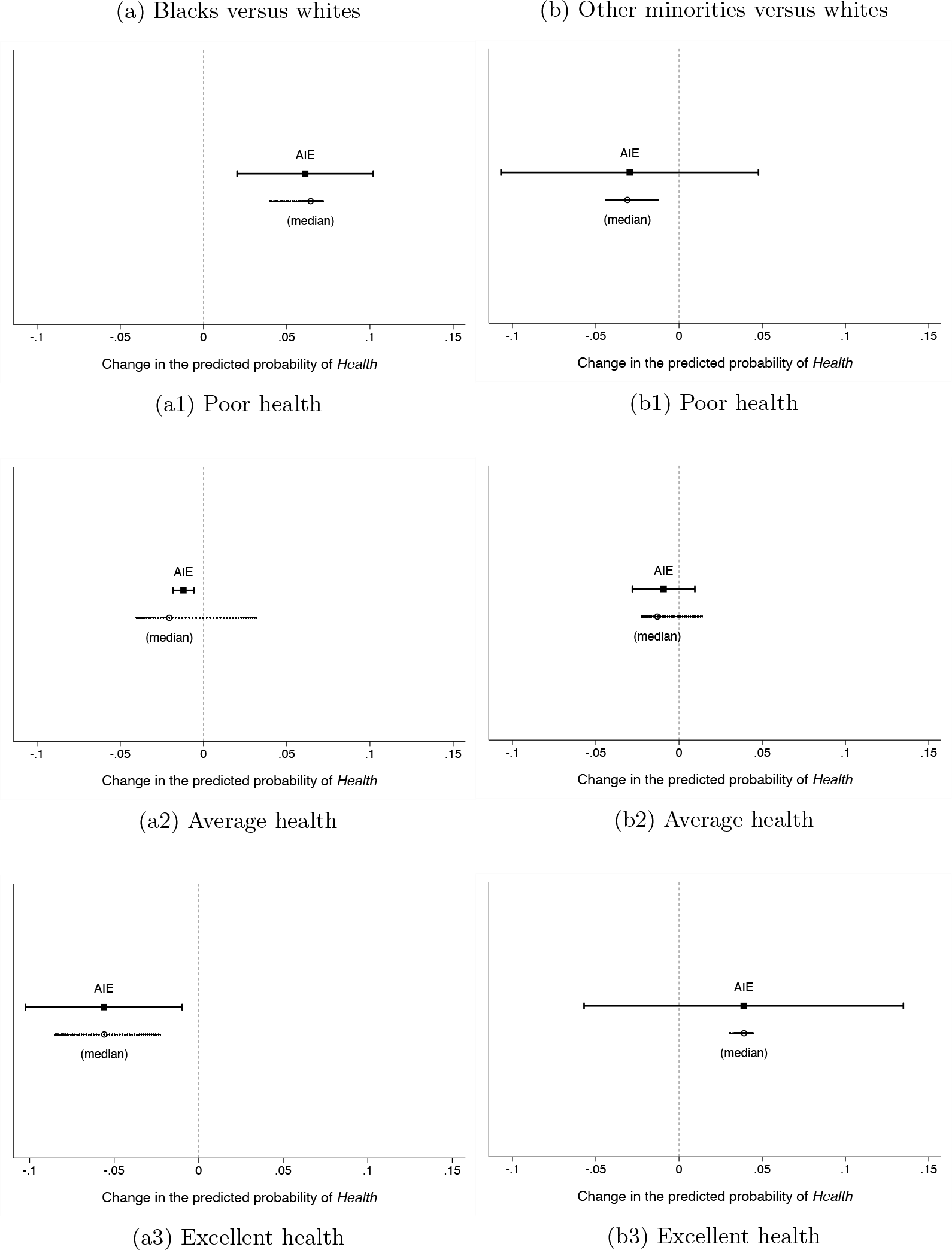
The interaction effect between gender and race on health (three-level indicator)

8 The interaction effect in practical applications

When assessing conditional hypotheses, researchers are typically interested in whether the treatment effect is constant across the levels of the moderator. The quantity of interest in such analyses is the interaction effect because it can provide the answer to the research question for linear and nonlinear models alike. Because of theoretical confusion or a lack of knowhow to compute the interaction effect, many analysts try to get at the interaction without computing the interaction effect. Resorting to heuristics or work-arounds, however, invites mistakes.

A common misconception is that we can draw valid inferences about the significance status of the interaction effect from the statistical significance level of the interaction term coefficient. In nonlinear models, however, a statistically significant interaction term is neither necessary nor sufficient for significant interactive effects. Conflating the interaction effect with the coefficient on the interaction term is another frequent misunderstanding. This is partly because, in a linear regression, the interaction effect is equal to the coefficient on the product term; that is, {∂Pr(y)}/(∂x ₁∂x ₂) = β _{x
₁} _{x
₂}. But this is not the case for nonlinear models.

Because of the erroneous association, questions about the coefficient on the interaction term are often misguided questions about the interaction effect. The many Statalist entries on this topic attest to how acute the problem is (for example, Statalist thread [2016, 2017a,b] to reference a few). Specifically, “[p]eople often ask what the ME [marginal effect] of an interaction term is […even though] there is not one” (Williams 2012, 329) and are willing to go to great lengths to obtain it.¹⁵ For example, to force an estimate for “the average marginal effect of the interaction,” one user proposed forgoing the Stata operator for interactions and manually generating the product between the interacted variables. Thus, instead of running the proper command

the user suggested the following work-around:

By defrauding margins into thinking that c is a real variable, one may obtain an estimate for its marginal effect, but, as Clyde Schechter succinctly put it, “[t]hat number is meaningless nonsense” (Statalist thread 2017a). After helpful comments and clarifications from Statalist contributors, it turns out the sought “effect of the interaction term” was actually the interaction effect.

With respect to the practical challenges of computing the interaction effect, some struggle to account for the simultaneous change in the second interacted variable. Let us look at a concrete example. Radean (2019) examines the interaction effect between office benefits and ideological preferences on the probability of party switching in Brazil. The dependent variable is coded 1 if a legislator who is a member of party A affiliates midterm with party B and 0 otherwise. President’s Coalition is coded 1 if the legislator’s party is a member of the president’s legislative coalition and 0 otherwise. This is taken as a proxy for access to state resources. Ideological Congruence is the distance between the legislator’s ideological position and that of the party.

Because President’s Coalition is a dummy variable, its effect is calculated as the discrete change from the base level. But is the effect constant across the range of ideological congruence? To answer this question, Radean (2019) reports the effect of President’s Coalition at minimum and maximum values of congruence with 84% CIs (see figure 1.Ia, 147). Unlike with the standard 95% CI, one can visually judge significance of differences at the 0.05 level from the overlap of the customized 84% intervals (Goldstein and Healy 1995; Schenker and Gentleman 2001). The use of this particular interval level, however, is appropriate only if the compared estimates are normally distributed, are independent (that is, not correlated), and have identical standard errors (Radean Forthcoming). These are very restrictive and unrealistic assumptions, and the study does not indicate whether all three conditions are simultaneously met. Using an imprecise interval level may, in turn, lead to incorrect inferences. Ultimately, from the information provided, we cannot determine whether the effect of office benefits changes as ideological congruence also changes.

The solution to all the problems discussed above is to compute the interaction effect—a task made easy by the ginteff command. Examining the interaction effect can lend additional support for the research hypothesis, but it may also provide evidence that contradicts it. Either way, the interaction effect should not be ignored.

8.1 Replication of a previous study

In this section, I illustrate one type of substantive findings that could be missed if researchers overlook the interaction effect. To do so, I replicate an analysis from Heller and Mershon (2005) on the effect of the electoral system and party discipline on party switching.¹⁶ The electoral system is made operational in terms of partyversus candidate-centered electoral rules. While the electorates vote for an individual candidate in candidate-centered electoral systems, they cast a party vote in party-centered systems (implicitly voting for all candidates on that party’s list). The Electoral Law variable is coded 1 if the legislator was elected under candidate-centered electoral rules and 0 if the legislator was elected on a party list.

Furthermore, the degree of party-label clarity (that is, information about the party’s policy stance) is used as a proxy for party discipline (that is, the control that party leaders exercise over the rank-and-file members). When party labels are clear, there is less uncertainty about the policy preference of party leadership. When the labels are blurry, legislators may sometimes find themselves at odds with their party’s position. Thus, leaders of parties with blurry labels have to enforce party discipline more frequently, which increases a legislator’s incentives to switch.

In terms of theoretical expectations, representatives elected under candidate-centered rules should be less likely to switch. Because voters can single them out on the ballot at the next election, they have higher incentives to keep faith with the electorate. By contrast, legislators elected on (closed) party lists are to some extent insulated from voter retribution. The underlying assumption here is that the electorate prefers loyal representatives, who do not jump ship when a better offer comes along. The negative effect of candidate-centered rules on the probability of party switching should be more pronounced in the context of clear party labels because the costs of strict party discipline are less onerous in this context (Heller and Mershon 2005, 538–539).

The output below replicates the logistic regression from Heller and Mershon (see model 3, table 4, 550). With a p-value of 0.274, the coefficient on the interaction term is far from the conventional levels of statistical significance. Based on this information, the authors infer that there is little empirical support for the conditional hypothesis and do not investigate further. Specifically, they do not compute either the marginal effect of the electoral system or the interaction effect.¹⁷

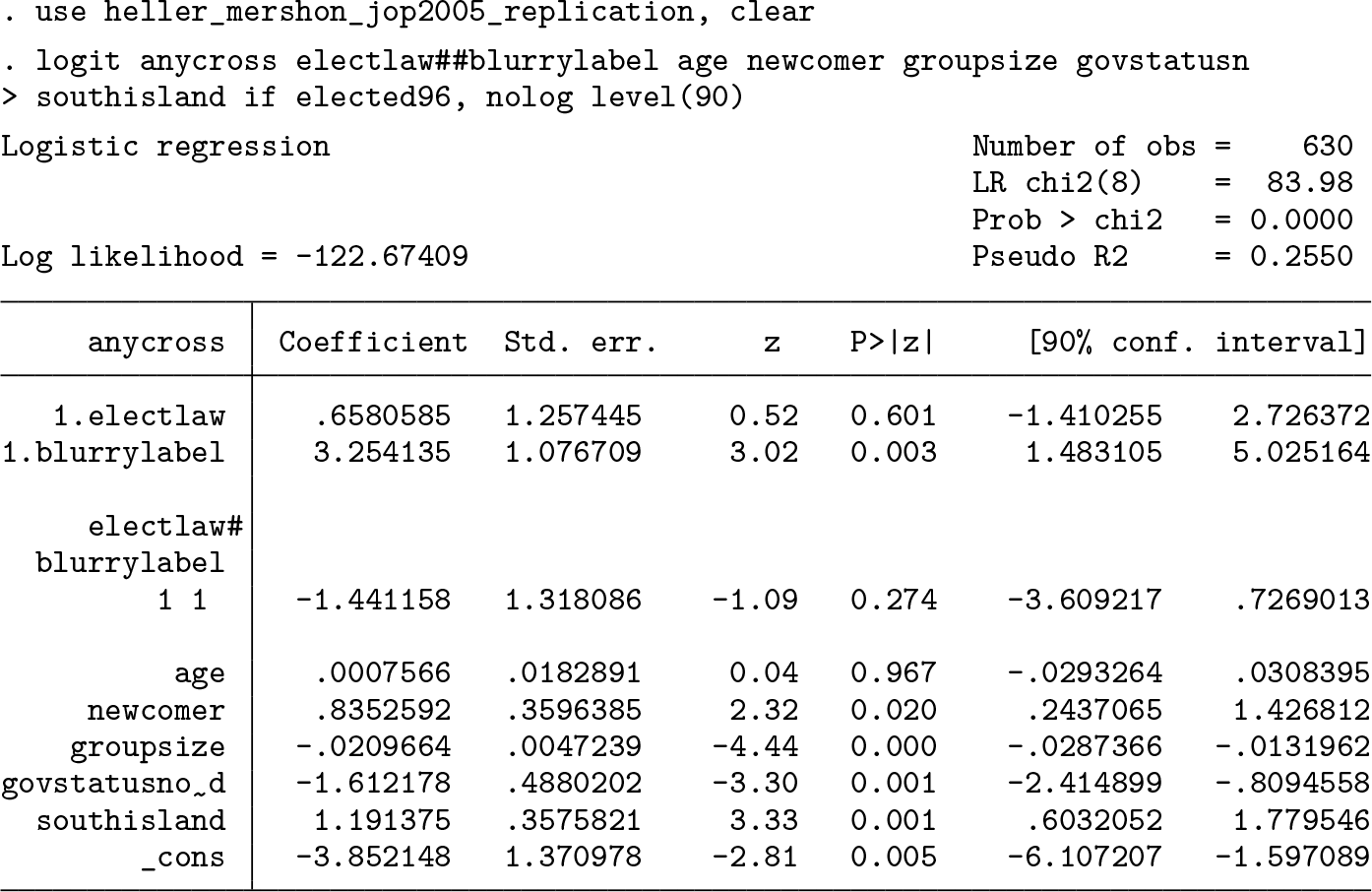
But, in a logit model, a statistically significant interaction term is not necessary for significant interactive effects (Ai and Norton 2003; Berry, DeMeritt, and Esarey 2010). To elucidate the matter, I first compute the marginal effect of the electoral system for both types of party labels using the margins command. These results are plotted in figure 4a. The effect is positive in the clear label scenario, suggesting that legislators elected under candidate-centered rules are more likely to switch than their party-list counterparts. As the authors note, this result does not support the theory, but the effect is also not statistically significant. The marginal effect of the electoral system is negative and significant in the blurry label scenario, which is in line with the theoretical expectation. While now we have a better idea of the conditional effect of the electoral system on party switching, we still cannot tell whether the effect is statistically different between the two scenarios. This is because the estimates’ CIs overlap. For a definitive answer, I compute the interaction effect using the ginteff command.

Figure 4.

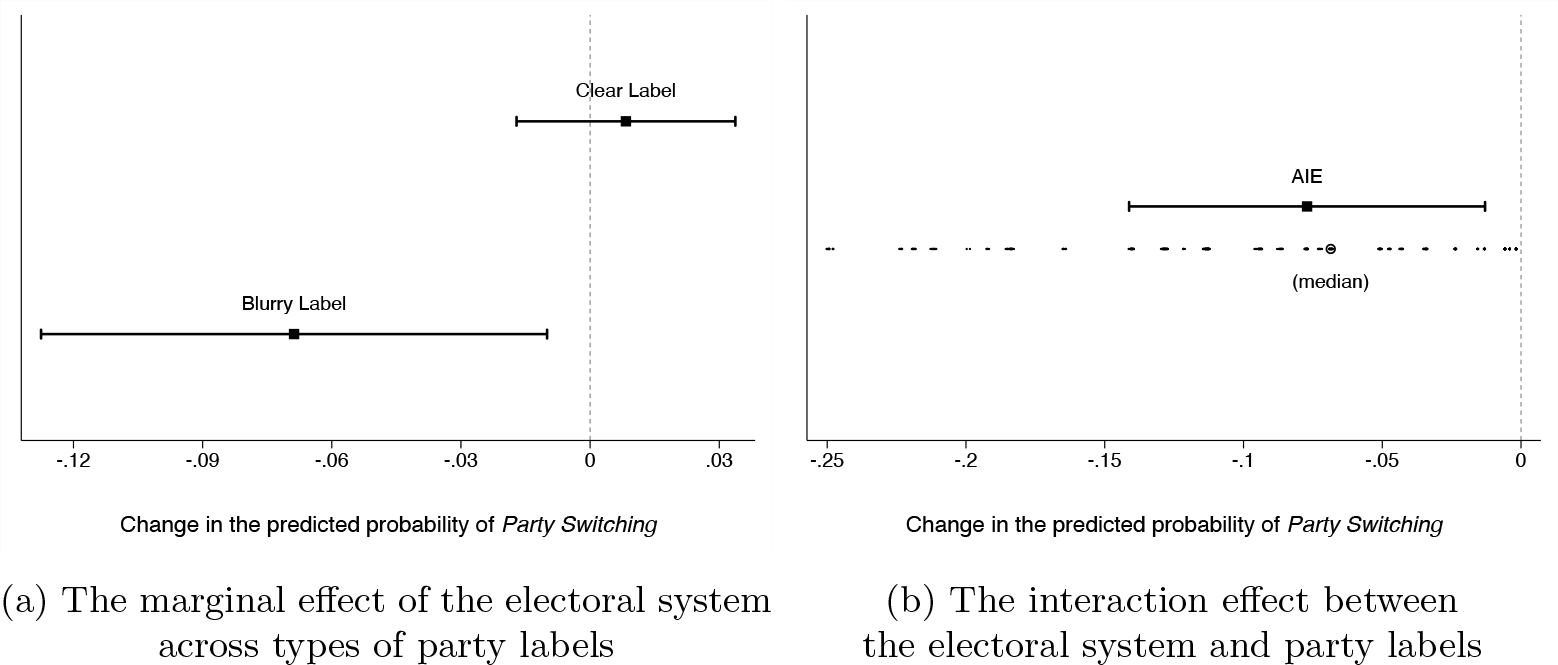
The effect of the electoral system on party switching

The statistically significant interaction effect (graphed in figure 4b) indicates that the effect of the electoral system on party switching is in fact distinct between clear and blurry party-label scenarios. Thus, the authors were too quick to dismiss the idea that party-label clarity conditions the effect of electoral rules. This is a piece of information that cannot be gleaned from either the logit coefficients or the conditional effects. More generally, there are cases where only by computing the interaction effect can we ascertain whether the treatment effect varies significantly with the levels of the moderator. In sum, by overlooking the interaction effect, we ignore crucial evidence for testing conditional hypotheses, which can lead to us either understating or, more problematically, overstating the extent of the empirical support for our theories.

8.2 Alternative approaches for continuous-by-continuous interactions

Besides computing the interaction effect, there are other options to explore how two continuous variables interact. One alternative is to plot the marginal effect of x ₁ across the range of the moderating variable x ₂, [Pr(y|x ₁ + n; x ₂ = min) − Pr(y|x ₁; x ₂ = min)] ,…, [Pr(y|x ₁ + n; x ₂ = max)] − Pr(y|x ₁; x ₂ = max) (see Brambor, Clark, and Golder [2006]). Marginal-effect graphs are useful for outlining the trajectory of the conditional effect but are not designed to compare the effect of x ₁ at alternative values of x ₂. Specifically, if there is overlap between the CIs of the effect of x ₁ at the minimum and maximum values of x ₂, we cannot tell whether the effect changes significantly with x ₂.

To illustrate the problem, let us consider a logistic regression with a dummy health indicator and a continuous-by-continuous interaction between height and weight.¹⁸ Figure 5a graphs the effect on health of increasing height by one standard deviation from its observed values across the range of weight. As expected, an increase in height always has a positive effect on health but more so for heavier people. This is because it decreases the body mass index by a greater amount. However, we cannot tell whether the effect of the counterfactual increase in height is statistically different between the minimum and maximum values of weight, because the associated 95% CIs overlap.

Figure 5.

Examining continuous-by-continuous interactions

Heat maps are another popular approach to examine continuous-by-continuous interactions (see Huber [2017]). This type of plot graphs the predicted probability of y across the range of both x ₁ and x ₂. The benefit of such graphs is that they cover a wide range of feasible values. Because no individual probabilities are identified, though, heat maps do not typically reveal the estimated uncertainty. Thus, we cannot judge whether a given change in predicted probability is statistically significant. Illustrating this problem, figure 5b graphs the predicted probability of being healthy across the range of both height and weight. It is easy to note that one has the lowest probability of being in good health when one scores low on height and high on weight (a scenario associated with a high body mass index). Conversely, higher probabilities are associated with low weight and high height scores. That said, from this graph we cannot tell whether Pr(health = 1 | height = max; weight = min) is statistically different from Pr(health = 1 | height = min; weight = max).

Unlike other empirical approaches, the interaction effect allows us to directly assess whether the change in the effect of x ₁ due to x ₂ also changing is statistically significant. Thus, it can be used to assess interactive theories. In fact, establishing whether the treatment effect is distinct at different values of the moderator is the crux of conditional hypothesis testing.

9 Conclusion

Interaction analyses are useful tools to examine complex socioeconomic outcomes where the effect of one variable depends on the presence or levels of another variable. Interaction effects capture the simultaneous change in two (or more) covariates, and their computation is challenging for models with a nonlinear link function (for example, binomial logit or probit) or models involving auxiliary parameters (for example, the correlation parameter in bivariate probit, the cutpoints in ordered logit, etc.). To complicate matters, in nonlinear analyses, the coefficient on the interaction term does not tell us the direction, magnitude, or significance of the interaction effect. For analyses where the interaction effect cannot be inferred from the model estimates, I introduce a new command that automatically computes two- and three-way interaction effects.

ginteff accommodates a large suite of estimation models and allows researchers to use either the partial derivative or the first difference to model the effect of the interacted variables. While ginteff is a specialized command, its many options make it fairly flexible. For example, a general concern with nonlinear models is that there is no one single effect, be it conditional or unconditional. In such instances, one can use the at() option to specify any number of relevant scenarios or compute the interaction effect for each observation via obseff().

Last, it is important to acknowledge that ginteff is a postestimation command in that it retrieves information from a regression model for further analysis but does not produce new estimates as such. This means that the ginteff results are only as good as the data fed into the command. In particular, ginteff assumes that the multiplicative model is correctly specified. For example, all constitutive terms are included (see Brambor, Clark, and Golder [2006]), there are no unmodeled interaction or quadratic terms, the underlying model assumptions hold, etc.

Concerning unmodeled terms, Beiser-McGrath and Beiser-McGrath (2020) show that omitted product terms can bias the included terms.¹⁹ As a possible solution, the study considers a suite of parametric and nonparametric estimators (that is, the adaptive lasso, kernel regularized least squares, and Bayesian additive regression trees). The advantage of these estimators is that they can select the covariates that belong in the model from a very large set of potential controls without leading to overfitting. One drawback is that they are more conservative; that is, the CI of relevant terms more frequently includes zero (729). Based on Monte Carlo simulations, the authors conclude that, on average, the adaptive lasso is the best approach. If using an alternative estimator, the analyst has to compute the interaction effect by hand while accounting for any constraints associated with that estimator.²⁰ If the results from the alternative estimator and those from the standard model are substantively similar (that is, there are no omitted relevant terms), researchers may use ginteff to compute the interaction effect using the estimates from the standard model.

Many researchers take for granted that model assumptions hold in their particular application without assessing the validity of these assumptions. But, when this is not the case, the estimates may be fragile and model dependent. This in turn can lead to incorrect inferences. Hainmueller, Mummolo, and Xu (2019) show that this is so even for the more innocuous case of linear regression. Specifically, the authors consider two common assumptions: 1) the linear interaction effect changes at a constant rate with the moderator, and 2) there is sufficient common support in the data to compute valid conditional effects. Based on a literature survey, they find that these assumptions often fail in practice, so they propose some diagnostics. A binning estimator (where a continuous moderator is broken into several bins) can provide a sense of the effect heterogeneity. It may also alert the analyst if the data are sparse. Another diagnostic tool is the kernel smoothing estimator. This estimation strategy relaxes the linearity assumption and estimates a flexible functional form of the treatment effect across the moderator’s range. If the diagnostic tests reveal that model assumptions hold, the research can compute the interaction effect using ginteff. If not, the analyst needs to first address the underlying problem.

Even if we have the appropriate research design and our model is correctly specified, we still need to exercise caution when computing substantive quantities of interest. We often make assumptions not only at the estimation stage but also in the postestimation phase. The latter type of assumption may be underappreciated but is equally important to obtain practically meaningful estimates. As an example, consider the oft-used fixed-effects logit model, which can be easily fit in Stata via the xtlogit command with the fe option. The standard panel-data model is

\Pr (y_{i t} = 1 ∣ x_{i t}, α_{i}) = \frac{e^{β x_{i t} + α_{i}}}{1 + e^{β x_{i t} + α_{i}}}, i = 1, \dots, N, t = 1, \dots, T_{i}

where (e^β)/(1 + e^β) is the standard logistic cumulative distribution function, α_i is the individual effect, i indexes individuals, and T_i is the number of observations on each individual. Fixed-effects models are attractive because they can account for time-invariant, unobserved individual characteristics. This in turn minimizes the risk that the coefficients on the observed predictors (the βs) are affected by the omitted variable bias. The downside is that we cannot make valid inferences about quantities of interest that require estimates of the fixed effects. The problem is that it is not possible to estimate α_i consistently when T_i is fixed (for a formal discussion, see Greene [2004, 106]). Providing the intuition for why adding more data cannot solve the problem, Wooldridge (2020, 467) explicates that “as we add each additional cross-sectional observation, we add a new α_i. No information accumulates on each α_i when T is fixed.”

This means we cannot compute predicted probabilities or partial effects unless we choose an arbitrary value for α. There is no optimal a priori value “[b]ecause the distribution of α_i is unrestricted—in particular, E(α_i) is not necessarily zero” (Wooldridge 2010, 558).²¹ But this is exactly what is typically assumed. Case in point, the margins command assumes α_i = 0 for every i when used after xtlogit with the fe option.²² Some analysts forcefully advise against calculating partial effects at α_i = 0 because estimates computed using an arbitrary value are not particularly meaningful (Baetschmann et al. 2020; Santos Silva and Kemp 2016). Because ginteff draws on calculations from margins, all assumptions are carried over. While evaluations of how problematic a particular assumption is are bound to be subjective, at the very least researchers should be aware of the assumptions made in the estimation and postestimation phases.

11 Programs and supplemental materials

Supplemental Material, sj-zip-1-stj-10.1177_1536867X231175253 - ginteff: A generalized command for computing interaction effects

Supplemental Material, sj-zip-1-stj-10.1177_1536867X231175253 for ginteff: A generalized command for computing interaction effects by Marius Radean in The Stata Journal

Footnotes

10 Acknowledgments

The author thanks Daina Chiba, the editor of the Stata Journal, and an anonymous reviewer for helpful comments and suggestions.

11 Programs and supplemental materials

To install a snapshot of the corresponding software files as they existed at the time of publication of this article, type

The User’s manuals and online appendix mentioned in the text can be found by installing these files.

For additional information as well as any future software updates, visit .

Notes

References

Norton

E. C.

2003. Interaction terms in logit and probit models. Economics Letters 80: 123–129. https://doi.org/10.1016/S0165-1765(03)00032-6.

Baetschmann

Ballantyne

Staub

K. E.

Winkelmann

2020. feologit: A new command for fitting fixed-effects ordered logit models. Stata Journal 20: 253–275. https://doi.org/10.1177/1536867X20930984.

Beiser-McGrath

L. F.

2020. Problems with products? Control strategies for models with interaction and quadratic effects. Political Science Research and Methods 8: 707–730. https://doi.org/10.1017/psrm.2020.17.

Berry

W. D.

DeMeritt

J. H. R.

Esarey

2010. Testing for interaction in binary logit and probit models: Is a product term essential? American Journal of Political Science 54: 248–266. https://doi.org/10.1111/j.1540-5907.2009.00429.x.

Brambor

Clark

Golder

2006. Understanding interaction models: Improving empirical analyses. Political Analysis 14: 63–82. https://doi.org/10.1093/pan/mpi014.

Cameron

A. C.

Trivedi

P. K.

2022. Microeconometrics Using Stata. 2nd ed. College Station, TX: Stata Press.

Clark

W. R.

Golder

2023. An Introduction to Interaction Models. Unpublished manuscript, Pennsylvania State University.

Cornelißen

Sonderhof

2009. Partial effects in probit and logit models with a triple dummy-variable interaction term. Stata Journal 9: 571–583. https://doi.org/10.1177/1536867X0900900404.

Gelman

Stern

2006. The difference between “significant” and “not significant” is not itself statistically significant. American Statistician 60: 328–331. https://doi.org/10.1198/000313006X152649.

10.

Goldstein

Healy

M. J. R.

1995. The graphical presentation of a collection of means. Journal of the Royal Statistical Society, Series A 158: 175–177. https://doi.org/10.2307/2983411.

11.

Greene

2004. The behaviour of the maximum likelihood estimator of limited dependent variable models in the presence of fixed effects. Econometrics Journal 7: 98–119. https://doi.org/10.1111/j.1368-423X.2004.00123.x.

12.

Hainmueller

Mummolo

2019. How much should we trust estimates from multiplicative interaction models? Simple tools to improve empirical practice. Political Analysis 27: 163–192. https://doi.org/10.1017/pan.2018.46.

13.

Heller

W. B.

Mershon

2005. Party switching in the Italian Chamber of Deputies, 1996–2001. Journal of Politics 67: 536–559. https://doi.org/10.1111/j.1468-2508.2005.00328.x.

14.

Huber

2017. In the spotlight: Visualizing continuous-by-continuous interactions with margins and twoway contour. Stata News, vol. 32, no. 1. https://www.stata.com/stata-news/news32-1/spotlight/.

15.

Kam

C. D.

Franzese

Jr . 2007. Modeling and Interpreting Interactive Hypotheses in Regression Analysis. Ann Arbor, MI: University of Michigan Press.

16.

Norton

E. C.

Wang

2004. Computing interaction effects and standard errors in logit and probit models. Stata Journal 4: 154–167. https://doi.org/10.1177/1536867X0400400206.

17.

Pinzon

2016. Effects of nonlinear models with interactions of discrete and continuous variables: Estimating, graphing, and interpreting. The Stata Blog: Not Elsewhere Classified. https://blog.stata.com/2016/07/12/effects-for-nonlinear-models-with-interactions-of-discrete-and-continuousvariables-estimating-graphing-and-interpreting/.

18.

Radean

2019. Sometimes you cannot have it all: Party switching and affiliation motivations as substitutes. Party Politics 25: 140–152. https://doi.org/10.1177/1354068816688363.

19.

Radean

. Forthcoming. The significance of differences interval: Assessing the statistical and substantive difference between two quantities of interest. Journal of Politics. https://doi.org/10.1086/723999.

20.

Santos Silva

J. M. C.

Kemp

G. C. R.

2016. Partial effects in fixed effects models. U.K. Stata Users Group meeting proceedings. https://www.stata.com/meeting/uk16/slides/santos_uk16.pdf.

21.

Schenker

Gentleman

J. F.

2001. On judging the significance of differences by examining the overlap between confidence intervals. American Statistician 55: 182–186. https://doi.org/10.1198/000313001317097960.

22.

StataCorp. 2021a. Stata 17 Lasso Reference Manual. College Station, TX.

23.

StataCorp. 2021b. Stata 17 Longitudinal-Data/Panel-Data Reference Manual. College Station, TX.

24.

Statalist thread (The Stata Forum) 2016. Statalist forums: Continuous interaction variables and margins. https://www.statalist.org/forums/forum/general-statadiscussion/general/1324886-continuous-interaction-variables-and-margins.

25.

Statalist thread (The Stata Forum) 2017a. Statalist forums: Marginal effect of interaction variable in probit regression using Stata. https://www.statalist.org/forums/forum/generalstata-discussion/general/1379890-marginal-effect-of-interaction-variable-in-probitregression-using-stata.

26.

Statalist thread (The Stata Forum) 2017b. Statalist forums: The margin effect of interaction term in nonlinear model (e.g. xtgee, family(binomial) link(probit)). https://www.statalist.org/forums/forum/general-stata-discussion/general/1379888-the-margin-effect-of-interactionterm-in-nonlinear-model-e-g-xtgee-family-binomial-link-probit.

27.

Wiggins

2004. Statalist archive: Re: st: Obtaining marginal effects and their standard errors after estimations with interactions. https://www.stata.com/statalist/archive/2013-01/msg00293.html.

28.

Williams

2012. Using the margins command to estimate and interpret adjusted predictions and marginal effects. Stata Journal 12: 308–331. https://doi.org/10.1177/1536867X1201200209.

29.

Williams

2021. Marginal effects for continuous variables. University of Notre Dame. https://www3.nd.edu/∼rwilliam/stats3/Margins02.pdf.

30.

Wooldridge

J. M.

2010. Econometric Analysis of Cross Section and Panel Data. 2nd ed. Cambridge, MA: MIT Press.

31.

Wooldridge

2020. Introductory Econometrics: A Modern Approach. 7th ed. Boston: Cengage Learning.

Supplementary Material

Please find the following supplemental material available below.

For Open Access articles published under a Creative Commons License, all supplemental material carries the same license as the article it is associated with.

For non-Open Access articles published, all supplemental material carries a non-exclusive license, and permission requests for re-use of supplemental material or any part of supplemental material shall be sent directly to the copyright owner as specified in the copyright notice associated with the article.

7.36 MB

0.00 MB