Sage Journals: Discover world-class research

Abstract

In this article, we introduce the xtivdfreg command, which implements a general instrumental-variables (IV) approach for fitting panel-data models with many time-series observations, T, and unobserved common factors or interactive effects, as developed by Norkute et al. (2021, Journal of Econometrics 220: 416–446) and Cui et al. (2020a, ISER Discussion Paper 1101). The underlying idea of this approach is to project out the common factors from exogenous covariates using principal-components analysis and to run IV regression in both of two stages, using defactored covariates as instruments. The resulting two-stage IV estimator is valid for models with homogeneous or heterogeneous slope coefficients and has several advantages relative to existing popular approaches.

In addition, the xtivdfreg command extends the two-stage IV approach in two major ways. First, the algorithm accommodates estimation of unbalanced panels. Second, the algorithm permits a flexible specification of instruments.

We show that when one imposes zero factors, the xtivdfreg command can replicate the results of the popular Stata ivregress command. Notably, unlike ivregress, xtivdfreg permits estimation of the two-way error-components paneldata model with heterogeneous slope coefficients.

Keywords

st0650 xtivdfreg xtivdfreg postestimation two-stage instrumental-variable estimation common factors interactive effects defactoring cross-sectional dependence two-way error-components panel-data model heterogeneous slope coefficients

1 Introduction

The common factor approach is highly popular among panel-data practitioners because it offers a wide scope for controlling for omitted variables and rich sources of unobserved heterogeneity, including models with cross-sectional dependence; see, for example, Chudik and Pesaran (2015), Juodis and Sarafidis (2018), and Sarafidis and Wansbeek (2012, 2021).

For panels where both of the cross-sectional and time-series dimensions (N and T, respectively) tend to be large, popular estimation approaches have been developed by Pesaran (2006) and Bai (2009) known in the literature as common correlated effects (CCE) and iterative principal components (IPC). Both methods involve least squares and project out the common factors using either cross-sectional averages of observables or principal-components analysis (PCA). To date, CCE and IPC have been applied to a large range of empirical areas and have been extended to several additional theoretical settings; see, for example, Su and Jin (2012), Moon and Weidner (2015, 2017), Baltagi, Ka, and Wang (2021), Harding, Lamarche, and Pesaran (2020), Kapetanios, Serlenga, and Shin (2021), and Li, Cui, and Lu (2020), among others.

Recently, Norkute et al. (2021) and Cui et al. (2020) developed a general instrumental-variables (IV) approach for estimating panel regressions with unobserved common factors when N and T are both large. The underlying idea is to project out the common factors from exogenous covariates using PCA and to construct instruments from defactored covariates. This first-stage IV (1SIV) estimator is consistent. In a second stage, the entire model is defactored based on factors extracted from the first-stage residuals, and IV regression is implemented again using the same instruments.

The resulting two-stage instrumental-variables (2SIV) approach combines features from both Pesaran (2006) and Bai (2009). In particular, following Pesaran (2006), the covariates of the model are assumed to be subject to a linear common factor structure. However, following Bai (2009), the common factors are projected out using PCA rather than cross-sectional averages. A major distinctive feature of 2SIV is that it eliminates the common factors from the error term and the regressors separately in two stages. In comparison, CCE eliminates the factors from the error and the regressors jointly, whereas IPC eliminates only the factors in the error.

2SIV is appealing for several reasons. First, CCE and IPC suffer from incidental parameters bias because an increasing number of parameters needs to be estimated as either T or N grows; see Westerlund and Urbain (2015) and Juodis, Karabiyik, and Westerlund (2021). Therefore, bias correction is required to ensure that inferences remain valid asymptotically. In contrast, 2SIV does not require bias correction in either dimension. This property is important because approximate procedures aiming to recenter the limiting distribution of particular estimators may not be able to fully eliminate all bias terms, especially those of high order; in such cases, substantial size distortions can occur in finite samples. Second, the CCE approach requires the so-called rank condition, which assumes that the number of factors does not exceed the rank of the (unknown) matrix of cross-sectional averages of the unobserved factor loadings. 2SIV does not require such a condition because the factors are estimated using PCA rather than cross-sectional averages. Third, the 2SIV objective function is linear in the parameters, and therefore the method is robust and computationally inexpensive.¹ In comparison, IPC relies on nonlinear optimization, and therefore convergence to the global optimum might not be guaranteed (Jiang et al. Forthcoming). Fourth, 2SIV shares a major attractive feature of CCE over IPC because it permits estimation of panels with heterogeneous slope coefficients. Last, 2SIV allows for endogenous regressors, so long as external instruments are available.

In this article, we introduce a new command, xtivdfreg, that implements the 2SIV approach and extends it in two major ways. First, the algorithm accommodates estimation of unbalanced panels. To achieve this, we use a variant of the expectationmaximization approach proposed by Stock and Watson (1998) and Bai, Liao, and Yang (2015). Second, the algorithm permits a flexible specification of instruments. In particular, it accommodates cases where 1) the covariates are driven by entirely different factors; 2) the covariates have a different number of factors, including no factors at all; and 3) different lags of defactored covariates are used as instruments.

We show that when one imposes zero factors and requests the 1SIV estimator, the xtivdfreg command can replicate the results of the popular ivregress command. Essentially, the two-stage least-squares (2SLS) estimator of the two-way error-components panel-data model can be viewed as a special case of the proposed 2SIV approach in that the former does not defactor the instruments. Notably, unlike ivregress, xtivdfreg permits estimation of the two-way error-components panel-data model with heterogeneous slope coefficients.

We illustrate the method with two examples. First, we use a panel dataset consisting of 300 U.S. financial institutions, each one observed over 56 time periods. We attempt to shed some light on the determinants of banks’ capital adequacy ratios. The results are compared with those obtained by using popular panel methods, such as the fixed-effects and 2SLS estimators, as well as the CCE estimator of Pesaran (2006). In the second example, we use macrodata used by Eberhardt and Teal (2010) for the estimation of cross-country production functions in the manufacturing sector. The dataset is unbalanced, containing observations on 48 developing and developed countries during the period 1970 to 2002.

The remainder of the article is organized as follows. Section 2, outlines the 2SIV approach developed by Norkute et al. (2021) and Cui et al. (2020) and discusses implementation with unbalanced panel data. Section 3 describes the syntax of the xtivdfreg command. Section 4 illustrates the command using real datasets. Section 5 concludes.

2 IV estimation of large panels with common factors

2.1 Models with homogeneous coefficients

We consider the following autoregressive distributed lag panel-data model with homogeneous slopes and a multifactor error structure:²

y_{i t} = α y_{i, t - 1} + β' x_{i t} + u_{i t}; i = 1, 2, \dots, N; t = 1, 2, \dots, T

and

u_{i t} = γ_{y, i}^{'} f_{y, t} + ε_{i t}

|α| < 1, β = (β ₁ , β ₂ ,…, β_K )′ such that at least one of ${β_{k}}_{k = 1}^{K}$ is nonzero, and X_it = ${(x_{i t}^{(1)}, x_{i t}^{(2)}, \dots, x_{i t}^{(K)})}^{'}$ is a K × 1 vector of regressors. The error term of the model is composite, where f _y,t and γ_y,i denote m_y × 1 vectors of true unobserved factors and factor loadings, respectively, and ε_it is an idiosyncratic error.

The vector of regressors x _it is assumed to be subject to the following data-generating process:³

x_{i t} = Γ_{x, i}^{'} f_{x, t} + v_{i t}

f _x,t denotes an m_x × 1 vector of true factors, Γ _x,i = (γ _1i , γ _2i ,…, γ_Ki ) denotes the corresponding m_x × K factor loading matrix, and v _it = (v_1it, v_2it ,…, v _Kit )′ is an idiosyncratic error term that is assumed to be independent from ε_it .⁴ Thus, x _it satisfies strict exogeneity with respect to ε_it , although it can be endogenous with respect to the total error term, u_it , via the factor component. This assumption ensures that one does not need to seek for external instruments. However, as discussed in remark 4, endogeneity with respect to ε_it can be allowed straightforwardly, provided there are valid external instruments available for estimation.

Stacking the T observations for each i yields

y_{i} = α y_{i,} {_{-}}_{1} + X_{i} β + u_{i}; u_{i} = F_{y} γ_{y, i} + ε_{i}

where y _i = (y _i ₁, y_i2,…, y_iT )′, y _i,−1 = L¹ y _i = (y_i0, y_i1,…, y_iT−1)′ with L^j defined as the jth lag operator, X _i = (x _i1, x _i2,…, x _iT )′ is T × K, u _i = (u_i1, u_i2,…, u_iT )′, F _y = (f _y,1, f _y,2,…, f _y,T )′ is T × m_y, and ε_i = (ε_i1, ε_i2,…, ε_iT )′. Similarly,

X_{i} = F_{x} Γ_{x, i} + V_{i}

where F _x = (f _x, ₁, f _x, ₂ ,…, f _x,T )′ is a T × m_x matrix and V _i = (v _i ₁, v _i ₂ ,…, v _iT )′ is T × K.⁵

Let W _i = (y _i,− ₁, X _i ) and θ = (α, β′)′. The model can be written more succinctly as

y_{i} = W_{i} θ + u_{i}

The 2SIV approach involves two stages. In the first stage, the common factors in X _i are asymptotically eliminated using PCA, and the defactored regressors are used as instruments to obtain consistent estimates of the structural parameters of the model, θ .

In the second stage, the entire model is defactored based on estimated factors extracted from the first-stage residuals, and another IV regression is implemented using the same instruments as in stage one.

2.1.1 First-stage IV estimator

Define ${\hat{F}}_{x}$ as $\sqrt{T}$ times the eigenvectors corresponding to the m_x largest eigenvalues of the T × T matrix $\sum_{i = 1}^{N} X_{i} X_{i}^{'} / N T$ . Also, let ${\hat{F}}_{x, - 1}$ denote a matrix defined similarly, except that it is based on $\sum_{i = 1}^{N} X_{i, - 1} X_{i, - 1}^{'} / N T$ , where X _i,− ₁ = L ¹ X _i .⁶

Consider the following empirical projection matrices:

M_{{\hat{F}}_{x}} = I_{T} - {\hat{F}}_{x} {({\hat{F}}_{x}^{'} {\hat{F}}_{x})}^{- 1} {\hat{F}}_{x}^{'}; M_{{\hat{F}}_{x, - 1}} = I_{T} - {\hat{F}}_{x, - 1} {({\hat{F}}_{x, - 1}^{'} {\hat{F}}_{x, - 1})}^{- 1} {\hat{F}}_{x, - 1}^{'}

In this case, the matrix of instruments can be formulated as

{\hat{Z}}_{i} = (M_{{\hat{F}}_{x}} X_{i}, M_{{\hat{F}}_{x, - 1}} X_{i, - 1})

which is of dimension T × 2K. Thus, the degree of overidentification of the model is 2K − (K + 1).

Remark 1. Further lags of X _i can be used as instruments straightforwardly. To illustrate, let q_z denote the total number of lags of X _i used as instruments, and define ${\hat{F}}_{x, - T}$ as $\sqrt{T}$ times the eigenvectors corresponding to the m_x largest eigenvalues of the T × T matrix $\sum_{i = 1}^{N} X_{i, - T} X_{i, - T}^{'} / N T$ , where X _i,−τ = L^τ X _i for τ = 1,…, q_z . The corresponding empirical projection matrices are of the same form as in (3) with ${\hat{F}}_{x, - 1}$ replaced by ${\hat{F}}_{x, - T}$ _. Moreover, in the case where the covariates are strictly exogenous, leads of X i can also be used as instruments; see remark 8 in section 4.1 for more details. In the absence of any lags of X _i (and further lags of y _i ) included in the model as regressors, the degree of overidentification is equal to q_zK − (K + 1).

The 1SIV estimator of θ is defined as

{\hat{θ}}_{1 SIV} = {({\hat{A}}_{N T}^{'} {\hat{B}}_{N T}^{- 1} {\hat{A}}_{N T})}^{- 1} {\hat{A}}_{N T}^{'} {\hat{B}}_{N T}^{- 1} {\hat{g}}_{N T}

where

{\hat{A}}_{N T} = \frac{1}{N T} \sum_{i = 1}^{N} {\hat{Z}}_{i}^{'} W_{i}; {\hat{B}}_{N T} = \frac{1}{N T} \sum_{i = 1}^{N} {\hat{Z}}_{i}^{'} {\hat{Z}}_{i}; {\hat{g}}_{N T} = \frac{1}{N T} \sum_{i = 1}^{N} {\hat{Z}}_{i}^{'} y_{i}

The 1SIV estimator is $\sqrt{N T}$ consistent; that is,

\sqrt{N T} ({\hat{θ}}_{1 SIV} - θ) = O_{p} (1)

as N and T grow jointly to infinity, that is, $(N, T) \overset{j}{\to} \infty$ , such that $N / T \to c, 0 < c < \infty$ . However, ${\hat{θ}}_{1 SIV}$ is asymptotically biased. Rather than bias correcting this estimator, Norkute et al. (2021) and Cui et al. (2020) put forward a second-stage estimator, which is free from asymptotic bias and is potentially more efficient. For this purpose, the first-stage estimator is useful because it provides a consistent estimate of the error term of the model, which is required to implement the second-stage IV estimator.

Remark 2. In the static panel case, where no lags of y _i are included on the right-hand side and the model is exactly identified (that is, no lags of the regressors are used as instruments), the 1SIV estimator reduces to

{\hat{θ}}_{1 SIV} = {(\sum_{i = 1}^{N} X_{i}^{'} M_{{\hat{F}}_{x}} X_{i})}^{- 1} \sum_{i = 1}^{N} X_{i}^{'} M_{{\hat{F}}_{x}} y_{i}

2.1.2 Second-stage IV estimator

To implement the second stage, extract estimates of the space spanned by F _y using residuals from the first stage; that is,

{\hat{u}}_{i} = y_{i} - W_{i} {\hat{θ}}_{1 SIV}

Subsequently, the entire model is defactored, and a second IV regression is run using the same instruments as in stage one.

In particular, let

M_{{\hat{F}}_{y}} = I_{T} - {\hat{F}}_{y} {({\hat{F}}_{y}^{'} {\hat{F}}_{y})}^{- 1} {\hat{F}}_{y}^{'}

where ${\hat{F}}_{y}$ is defined as $\sqrt{T}$ times the eigenvectors corresponding to the m_y largest eigenvalues of the T × T matrix $\sum_{i = 1}^{N} {\hat{u}}_{i} {\hat{u}}_{i}^{'} / N T$ .

The (optimal) second-stage IV estimator is defined as

{\hat{θ}}_{2 SIV} = {({\hat{\hat{A}}}_{N T}^{'} {\hat{\hat{Ω}}}_{N T}^{- 1} {\hat{\hat{A}}}_{N T})}^{- 1} {\hat{\hat{A}}}^{'}_{N T} {\hat{\hat{Ω}}}_{N T}^{- 1} {\hat{\hat{g}}}_{N T}

where

{\hat{\hat{A}}}_{N T} = \frac{1}{N T} \sum_{i = 1}^{N} {\hat{Z}}_{i}^{'} M_{{\hat{F}}_{y}} W_{i}; {\hat{\hat{g}}}_{N T} = \frac{1}{N T} \sum_{i = 1}^{N} {\hat{Z}}_{i}^{'} M_{{\hat{F}}_{y}} y_{i}

and

{\hat{\hat{Ω}}}_{N T} = \frac{1}{N T} \sum_{i = 1}^{N} {\hat{Z}}_{i}^{'} M_{{\hat{F}}_{y}} {\hat{u}}_{i} {\hat{u}}_{i}^{'} M_{{\hat{F}}_{y}} {\hat{Z}}_{i}

As shown by Norkute et al. (2021), ${\hat{θ}}_{1 SIV}$ is $\sqrt{N T}$ consistent and asymptotically

normally distributed, such that

\sqrt{N T} ({\hat{θ}}_{2 SIV} - θ) \overset{d}{\to} N {0, {(A^{'} Ω^{- 1} A)}^{- 1}}

as $(N, T) \overset{j}{\to} \infty$ with $N / T \to c, 0 < c < \infty$ ⁷

Notice that the limiting distribution of ${\hat{θ}}_{2 SIV}$ is correctly centered, and thus no bias correction is required. As demonstrated by Cui et al. (2020), the main intuition of this result lies in that F _x Γ _x,i is estimated from X _i , whereas F _yγ_y,i is estimated from u _i . Because V _i , F _yγ_y,i , and ε_i are independent from one another, any correlations that arise because of the estimation error of ${\hat{F}}_{y}$ and ${\hat{F}}_{x}$ are asymptotically negligible.

Remark 3. In the static panel case, where no lags of y _i are included on the right-hand side and the model is exactly identified, the second-stage IV estimator can be expressed as

{\hat{θ}}_{2 SIV} = {(\sum_{i = 1}^{N} X_{i}^{'} M_{{\hat{F}}_{x}} M_{{\hat{F}}_{y}} X_{i})}^{- 1} \sum_{i = 1}^{N} X_{i}^{'} M_{{\hat{F}}_{x}} M_{{\hat{F}}_{y}} y_{i}

In this case, proposition 3.2 in Cui et al. (2020) reveals that the second-stage estimator is asymptotically equivalent to a least-squares estimator obtained by regressing y _i− F _yγ_y,I on X _i − F _x Γ _x,i . Moreover, the authors show that ${\hat{θ}}_{2 SIV}$ is asymptotically as efficient as the bias-corrected CCE and IPC estimators.

Remark 4. The assumptions imposed thus far imply that X _i satisfies strict exogeneity with respect to ε_i because otherwise extracting principal components from X _i may be invalid. When some of the regressors are endogenous (or weakly exogenous) with respect to ε_it , 2SIV requires using external exogenous instruments.⁸ To illustrate, let X _i = (X _i ^(exog), X _i ^(endog)), where X _i ^(exog) and X _i ^(endog) refer to the strictly exogenous and endogenous regressors, respectively, which are of dimension T ×K ^(exog) and T ×K ^(endog). Furthermore, let X _i + = (X _i ^(exog), X _i ^(ext)), a T × K* matrix with K* = K ^(exog) + K ^(ext), where X _i ^(ext) denotes the matrix of external exogenous covariates. X _i ^(ext) can still be correlated with the factor component; that is, it may be subject to a similar datagenerating process as in (2). Define ${\hat{F}}_{x}^{+}$ as $\sqrt{T}$ times the eigenvectors corresponding to the $m_{x}^{+}$ largest eigenvalues of the T ×T matrix $\sum_{i = 1}^{N} X_{i}^{+} {(X_{i}^{+})}^{'} / N T$ . The corresponding projection matrices are defined in the same way as in (3) with ${\hat{F}}_{x}$ $({\hat{F}}_{x . - 1})$ replaced by ${\hat{F}}_{x}^{+}$ $({\hat{F}}_{_{x . - 1}}^{+})$ . In this case, the matrix of instruments becomes

{\hat{Z}}_{i} = (M_{{\hat{F}}_{x}^{+}} X_{i}^{+}, M_{{\hat{F}}_{x, - 1}^{+}} X_{i, - 1}^{+})

The overidentifying restrictions J-test statistic associated with the second-stage IV estimator is given by

J_{N T} = \frac{1}{N T} (\sum_{i = 1}^{N} {\hat{\hat{u}}}_{i}^{'} M_{{\hat{F}}_{y}} {\hat{Z}}_{i}) {\hat{\hat{Ω}}}_{N T}^{- 1} (\sum_{i = 1}^{N} {\hat{Z}}_{i}^{'} M_{{\hat{F}}_{y}} {\hat{\hat{u}}}_{i})

where ${\hat{\hat{u}}}_{i} = y_{i} - W_{i} {\hat{θ}}_{2 SIV}$ and ${\hat{\hat{Ω}}}_{N T}$ is defined in (7).

The overidentifying restrictions test is particularly useful in this approach. First, it is expected to pick up a violation of the exogeneity of the defactored covariates with respect to the idiosyncratic error in the equation for y _i . Second, the orthogonality condition of the instruments is violated if the slope vector, θ, is cross-sectionally heterogeneous. In this case, the estimators proposed in this section may become inconsistent, and the J test is expected to reject the null hypothesis asymptotically.

2.2 Models with heterogeneous coefficients

We now turn our focus on models with heterogeneous coefficients. Let

y_{i} = W_{i} θ_{i} + u_{i}

where $θ_{i} = {(α_{i}, β_{i}^{'})}^{'}$ with sup_1≤i≤N |α_i | < 1.

The IV estimator of θ_i is defined as

{\hat{θ}}_{IV, i} = {({\tilde{A}}_{i, T}^{'} {\tilde{B}}_{i, T}^{- 1} {\tilde{A}}_{i, T})}^{- 1} {\tilde{A}}_{i, T}^{'} {\tilde{B}}_{i, T}^{- 1} {\tilde{g}}_{i, T}

where

{\tilde{A}}_{i, T} = \frac{1}{T} {\hat{Z}}_{i}^{'} M_{{\hat{F}}_{x}} W_{i}; {\tilde{B}}_{i, T} = \frac{1}{T} {\hat{Z}}_{i}^{'} M_{{\hat{F}}_{x}} {\hat{Z}}_{i}; {\tilde{g}}_{i, T} = \frac{1}{T} {\hat{Z}}_{i}^{'} M_{{\hat{F}}_{x}} y_{i}

${\hat{z}}_{i}$ is defined in (4), and $M_{{\hat{F}}_{x}}$ is defined in (3) with ${\hat{F}}_{x}$ obtained as $\sqrt{T}$ times the eigenvectors corresponding to the m_x largest eigenvalues of the T ×T matrix $\sum_{i = 1}^{N} X_{i} X_{i}^{'} / N T$ .

The mean-group instrumental-variables (MGIV) estimator of θ is

{\hat{θ}}_{MGIV} = \frac{1}{N} \sum_{i = 1}^{N} {\hat{θ}}_{IV, i}

As shown by Norkute et al. (2021), as $(N, T) \overset{j}{\to} \infty$ such that N/T → c with 0 < c < ∞,

\sqrt{N} ({\hat{θ}}_{MGIV} - θ) \overset{d}{\to} N (0, Σ_{η})

and

{\hat{Σ}}_{η} - Σ_{η} \overset{p}{\to} 0

where

{\hat{Σ}}_{η} = \frac{1}{N - 1} \sum_{i = 1}^{N} ({\hat{θ}}_{IV, i} - {\hat{θ}}_{MGIV}) {({\hat{θ}}_{IV, i} - {\hat{θ}}_{MGIV})}^{'}

Note that the overidentifying restrictions test statistic is not valid for the model with heterogeneous coefficients.⁹

Remark 5. In the static panel case, where no lags of y _i are included on the right-hand side and the model is exactly identified, the individual-specific IV estimator reduces to

{\hat{θ}}_{IV, i} = {(X_{i}^{'} M_{{\hat{F}}_{x}} X_{i})}^{- 1} X_{i}^{'} M_{{\hat{F}}_{x}} y_{i}

Remark 6. When the model contains endogenous regressors, the matrices listed in (10) are given by

{\tilde{A}}_{i, T} = \frac{1}{T} {\hat{Z}}_{i}^{'} M_{{\hat{F}}_{x}^{+}} W_{i}; {\tilde{B}}_{i, T} = \frac{1}{T} {\hat{Z}}_{i}^{'} M_{{\hat{F}}_{x}^{+}} {\hat{Z}}_{i}; {\tilde{g}}_{i, T} = \frac{1}{T} {\hat{Z}}_{i}^{'} M_{{\hat{F}}_{x}} + y_{i}

where $\hat{Z_{i}}$ is defined in (8).

2.3 Unbalanced panels

When the panel-data model is unbalanced, that is, some observations are missing at random, our procedure needs to be modified to control for the unobserved common factors. Following Stock and Watson (1998) and Bai, Liao, and Yang (2015), we may distinguish between X _i and $X_{i}^{*}$ . $X_{i}^{*}$ is a T × K matrix containing the true values of the regressors, and it is defined as in (2). Let $x_{i, t}^{* (k)}$ denote the (t, k)th entry of $X_{i}^{*}$ , and $ι_{i, t}^{(k)}$ denote a binary indicator that takes the value unity if the kth variable for individual i at time t is observed and zero otherwise. Thus, we set $x_{i, t}^{(k)} = x_{i, t}^{* (k)} if ι_{i, t}^{(k)} = 1$ and $x_{i, t}^{(k)}$ is unobserved otherwise, k = 1,…, K.¹⁰

Let ${\hat{f}}_{x, t}^{(0)}$ and ${\hat{γ}}_{k i}^{(0)}$ denote some initial values for the factors and factor loadings, respectively. Also, let $\bar{T} = max {T_{1}, T_{2}, \dots, T_{N}}$ , where T_i denotes the maximum number of observations for individual i.

In the first iteration, the values of the regressors are set such that

{\hat{x}}_{i, t}^{(k, 1)} = {\begin{array}{l} x_{i, t}^{* (k)} & if & ι_{i, t}^{(k)} = 1 \\ {({\hat{f}}_{x, t}^{(0)})}^{'} {\hat{γ}}_{k i}^{(0)} & if & ι_{i, t}^{(k)} = 0 \end{array}

The factors in the first iteration, ${\hat{f}}_{x, t}^{(1)}$ , are extracted as $\sqrt{T}$ times the eigenvectors corresponding to the m_x largest eigenvalues of the matrix

V_{x}^{(1)} = \sum_{k = 1}^{K} \sum_{i = 1}^{N} {\hat{x}}_{i}^{(k, 1)} {({\hat{x}}_{i}^{(k, 1)})}^{'} / (N \bar{T})

where ${\hat{x}}_{i}^{(k, 1)} = {({\hat{x}}_{i, 1}^{(k, 1)}, {\hat{x}}_{i, 2}^{(k, 1)}, \dots, {\hat{x}}_{i, T}^{(k, 1)})}^{'}$ . The corresponding factor loadings, ${\hat{γ}}_{k i}^{(1)}$ , are the estimated individual-specific coefficients obtained by regressing ${\hat{x}}_{i, 1}^{(k, 1)}$ on ${\hat{f}}_{x, t}^{(1)}$ , k =1,…, K.

Subsequent iterations are based on

V_{x}^{(l)} = \sum_{k = 1}^{K} \sum_{i = 1}^{N} {\hat{x}}_{i}^{(k, l)} {({\hat{x}}_{i}^{(k, l)})}^{'} / (N \bar{T})

for ℓ > 1, until convergence. The convergence criterion is defined with respect to the objective function

V_{x}^{(l)} = {(N \bar{T})}^{- 1} \sum_{k = 1}^{K} \sum_{t = 1}^{T} \sum_{i = 1}^{N} {{\hat{x}}_{i t}^{(k, l)} - {({\hat{f}}_{x, t}^{(l)})}^{'} {\hat{γ}}_{k i}^{(l)}}^{2}

where ${\hat{x}}_{i t}^{(k, l)}$ denotes the estimated value of the kth regressor corresponding to the ℓth iteration for individual i at time t, while ${\hat{f}}_{x, t}^{(l)}$ and ${\hat{γ}}_{k i}^{(l)}$ are defined similarly as before.

The initial factor values are determined using a similar eigenvalue problem as outlined previously, this time based on x _i ^(k), a column vector of length $\bar{T}$ with missing values replaced by zeros. That is, ${\hat{f}}_{x, t}^{(0)}$ is computed as $\sqrt{T}$ times the eigenvectors corresponding to the m_x largest eigenvalues of the matrix

V_{x}^{(0)} = \sum_{k = 1}^{K} \sum_{i = 1}^{N} x_{i}^{(k)} {(x_{i}^{(k)})}^{'}

with the (j ₁ , j ₂) entry being divided by the number of summands used when this number is larger than zero.

The same procedure is followed when extracting factors from lagged values of X _i or from the residuals obtained from the first-stage estimation.¹¹

3 The xtivdfreg command

3.1 Syntax

xtivdfreg depvar [indepvars] [ if ] [ in ] , absorb(absvars)

iv( varlist , [fvar( fvars ) lags( # ) factmax( # ) [no] eigratio

[no] doubledefact ]) factmax(#) [no] eigratio [no] doubledefact fstage

iterate( # ) ltolerance( # ) nodots noconstant level( # ) coeflegend

noheader notable display_options ]

3.2 Options

absorb(absvars) specifies categorical variables that identify the fixed effects to be absorbed. Typical use is absorb(panelvar) or absorb(panelvar timevar) for one-way or two-way fixed effects, respectively.¹²

iv(varlist [ , [fvar(fvars) lags(#) factmax(#) [ no ] eigratio [ no ] doubledefact ) specifies IV. One can specify as many sets of instruments as required. Variables in the same set are defactored jointly. External variables that are not part of the regression model can also be used as instruments in varlist.

fvar(fvars) specifies that factors be extracted from the variables in fvars. The default is to extract factors from all variables in varlist.

lags(#) specifies the # of lags of varlist to be added to the set of instruments. The variables at each lag order are defactored separately with factors extracted from the corresponding lag of fvars. The default is lags(0).

factmax(#) specifies the maximum number of factors to be extracted from fvars. The default is set by the global option factmax(#).

noeigratio and eigratio request either to use a fixed number of factors as specified with the suboption factmax(#) or to use the Ahn and Horenstein (2013) eigenvalue ratio test to compute the number of factors. eigratio is the default unless otherwise specified with the global option noeigratio.

doubledefact requests to include fvars in a further defactorization stage of the entire model for the first-stage estimator. All sets of instruments that are included in this defactorization stage are jointly defactored, excluding lags of fvars specified with the suboption lags(#). nodoubledefact requests to avoid implementing a further defactorization stage of the entire model for the first-stage estimator. The default is set by the global option [no] doubledefact.

factmax(#) specifies the maximum number of factors for each estimation stage and each set of instruments. The default is factmax(4).

noeigratio requests to use a fixed number of factors as specified with the option factmax(#). By default, the eigenvalue ratio test of Ahn and Horenstein (2013) is used to compute the number of factors for each estimation stage and each set of instruments.

doubledefact requests to use a further defactorization stage of the entire model for the first-stage estimator, as, for example, described in footnote 7. nodoubledefact requests to avoid implementing this further defactorization stage. doubledefact is the default when the option mg is specified, and nodoubledefact is the default when the option mg is omitted.

fstage requests the 1SIV estimator to be computed instead of the second-stage IV estimator.

mg requests the mean-group estimator to be computed, which allows for heterogeneous slopes.

iterate(#) specifies the maximum number of iterations for the extraction of factors. If convergence is declared before this threshold is reached, it will stop when convergence is declared. The default is the number set using set maxiter. This option has no effect with strongly balanced panel data, in which case any iterations are redundant.

ltolerance(#) specifies the convergence tolerance for the objective function; see [R] Maximize. The default is ltolerance(1e-4). This option has no effect with strongly balanced panel data.

nodots requests not to display dots for the iteration steps. By default, one dot character is displayed for each iteration step. This option has no effect with strongly balanced panel data.

noconstant suppresses the constant term.

level(#), coeflegend; see [R] Estimation options.

noheader suppresses display of the header above the coefficient table that displays the number of observations and moment conditions.

notable suppresses display of the coefficient table.

display_options: noci, nopvalues, noomitted, vsquish, noemptycells, baselevels, allbaselevels, nofvlabel, fvwrap(#), fvwrapon(style), cformat(%fmt), pformat(%fmt), sformat(%fmt), and nolstretch; see [R] Estimation options.

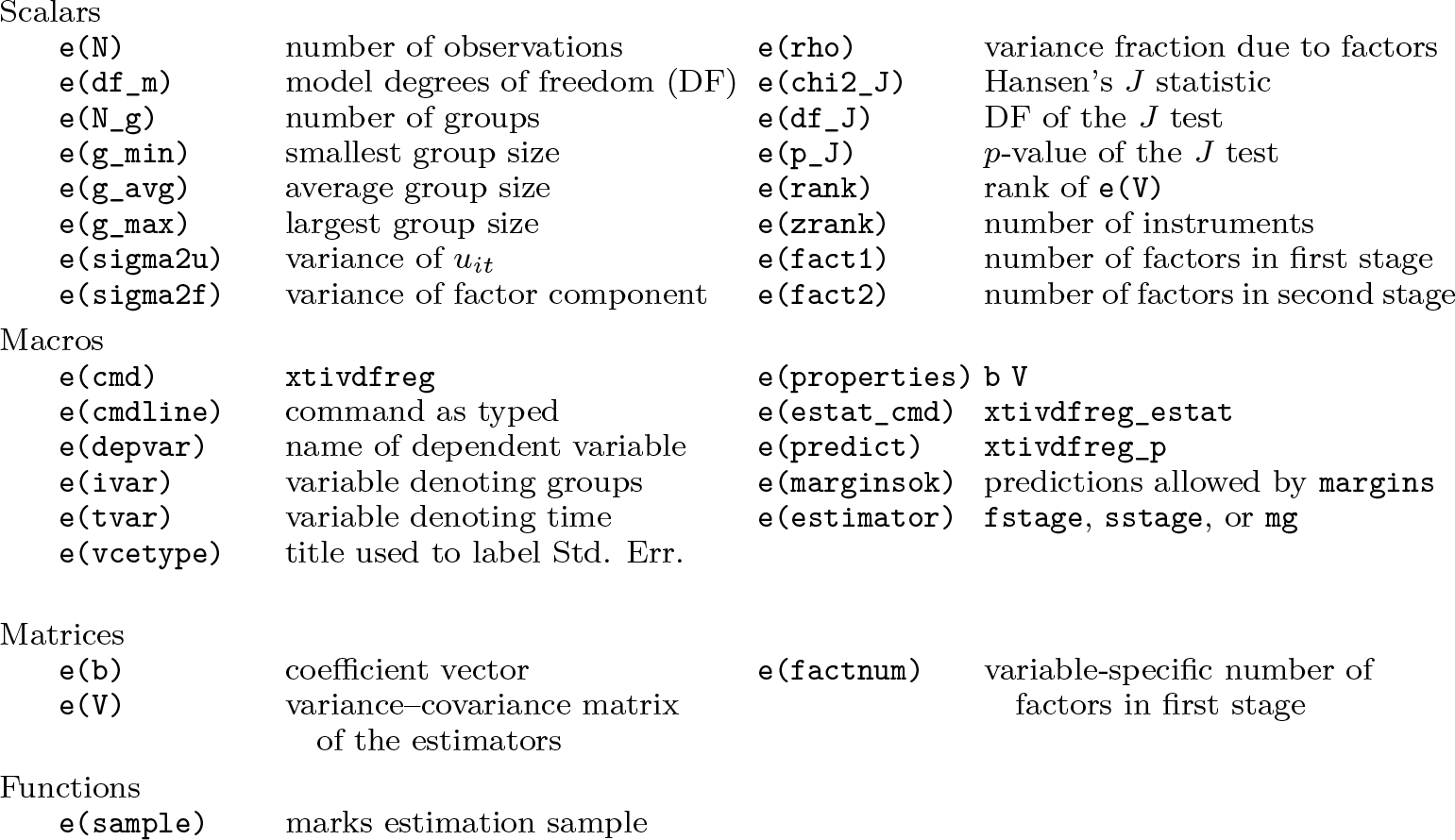
3.3 Stored results

xtivdfreg stores the following in e():

4 Examples

4.1 Example 1: Estimation of the determinants of banks’ capital adequacy ratios

In this example, we illustrate the xtivdfreg command by estimating the effect of main drivers behind capital adequacy ratios for banking institutions. We make use of panel data from a random sample of 300 U.S. banks, each one observed over 56 time periods, namely, 2006:Q1–2019:Q4.

We focus on the model

\begin{array}{l} {CAR}_{i t} = α {CAR}_{i t - 1} + β_{1} {size}_{i t} + β_{2} {ROA}_{i t} + β_{3} {liquidity}_{i t} + u_{i t} \\ u_{i t} = η_{i} + τ_{t} + γ_{y, i}^{'} f_{y, t} + ε_{i t} \end{array}

where i = 1,…, 300 and t = 2,…, 56. All data are publicly available, and they have been downloaded from the Federal Deposit Insurance Corporation website.¹³

CAR _it stands for “capital adequacy ratio”, which is proxied by the ratio of tier 1 (core) capital over risk-weighted assets.

size _it is proxied by the natural logarithm of banks’ total assets.

ROA _it stands for the “return on assets”, defined as annualized net income expressed as a percentage of average total assets. ROA is used as a measure of profitability.

liquidity _it is proxied by the loan-to-deposit ratio. Note that higher values of this variable imply a lower level of liquidity.

Finally, the error term is composite; η_i and τ_t capture bank-specific and time-specific effects, f _y,t is an m_y ×1 vector of unobserved common shocks with corresponding loadings given by γ_y,i , and ε_it is a purely idiosyncratic error. Note that m_y is unknown.

Some discussion on the interpretation of the parameters that characterize (12) is useful. The autoregressive coefficient, α, reflects costs of adjustment that prevent banks from achieving optimal levels of capital adequacy instantaneously. β_k , for k = 1,…, K(= 3), denote the slope coefficients of the model. β ₁ measures the effect of size on capital adequacy behavior. Under the “too-big-to-fail hypothesis”, large banks may count on public bailout during periods of financial distress, knowing that they are systematically very important (for example, Cui, Sarafidis, and Yamagata [2020b]). Essentially, this hypothesis reflects the classic moral hazard problem, where one party takes on excessive risk, knowing that it is protected against the risk and that another party will incur the cost. Under such a scenario, β ₁ is expected to be negative.

β ₂ measures the effect of profitability on capital adequacy. Standard theory suggests that higher bank profitability dissuades a bank’s risk taking, and thus it is associated with larger capital reserves because profitable banks stand to lose more shareholder value if downside risks realize (Keeley 1990). On the other hand, more profitable banks can borrow more and engage in risky activities on a larger scale under the presence of leverage constraints (Martynova, Ratnovski, and Vlahu 2020). A positive (negative) value of β ₂ is consistent with the former (latter) interpretation. Lastly, the direction of the effect of liquidity, β ₃, is ultimately an empirical question as well. For instance, a positive value indicates that lower liquidity levels force banks to increase their capital reserves, arguably to reduce risk exposure.

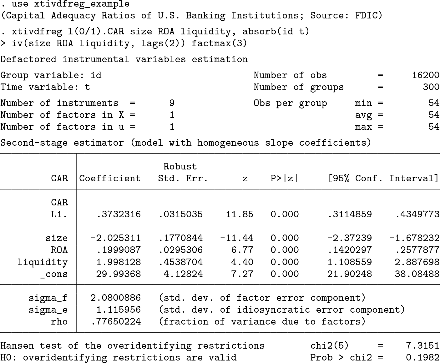
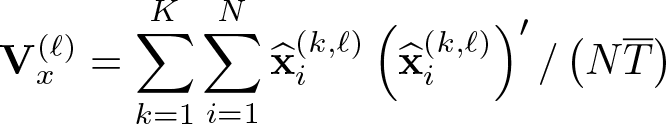
We start by running the xtivdfreg command using two lags of the covariates as defactored instruments and up to a maximum of three factors. Thus, we use nine instruments in total, three for each covariate. There are four parameters, which implies that the degree of overidentification equals five. We control for bank-specific and timespecific effects by eliminating them prior to estimation. This baseline regression is obtained as follows:

To illustrate the specification of the command in terms of the notation used in the article, let $X_{i} = (X_{i}^{(1)}, X_{i}^{(2)}, X_{i}^{(3)})$ , where $X_{i}^{(k)}$ denotes the regressor corresponding to the coefficient β_k in (12), for k = 1, 2, 3. The matrix of instruments is given by

{\hat{Z}}_{i} = (M_{{\hat{F}}_{x}} X_{i}, M_{{\hat{F}}_{x, - 1}} X_{i, - 1}, M_{{\hat{F}}_{x, - 2}} X_{i, - 2})

which is of dimension T × 3K, with ${\hat{F}}_{x, - τ}$ defined as $\sqrt{T}$ times the eigenvectors corresponding to the m_x largest eigenvalues of the T × T matrix $\sum_{i = 1}^{N} X_{i, - τ} X_{i, - τ}^{'} / N T$ , for τ = 1, 2. The second-stage IV estimator is defined in (6).

All coefficients are statistically significant at the 1% level. Moreover, the p-value of the J-test statistic suggests that the overidentifying restrictions (instruments) are valid. The estimated number of factors in the first and second stages equals 1 in both cases; that is, ${\hat{m}}_{x} = {\hat{m}}_{y} = 1$ .

xtivdfreg also reports the fraction of the variance of u_it that is explained by the factor component, denoted as rho. Because the value of rho is roughly equal to 3/4 in the present sample, it appears that most of the variation in the composite error term is due to the single unobserved factor, conditional on bank-specific and time-specific effects. Therefore, estimators that fail to control for common shocks are likely to be severely biased.

The estimated autoregressive coefficient equals about 0.373, which suggests medium persistence in the CAR time series. The estimated coefficient of size is highly negative, so it is consistent with the “too-big-to-fail hypothesis”, providing evidence of moral hazard-type behavior of banking institutions. Profitability (ROA) appears to have a positive effect on capital adequacy, which is in line with Keeley (1990). The positive estimate for β ₃ shows that lower levels of bank asset liquidity (that is, higher values of liquidity) lead to an increase in capital reserves, all other things being equal. This implies that banking institutions suffering from a liquidity crunch tend to respond by raising their equity.

Finally, note that xtivdfreg reports an estimate of a constant term (intercept). This is obtained as the mean of the residuals in a separate step after computing the slope coefficients.¹⁴ Whether a constant term is estimated has no effect on the computation of the slope coefficients because the latter are computed for the demeaned model with or without the absorption of fixed effects. The standard error of the constant term is computed with the influence-function approach of Kripfganz and Schwarz (2019).

Next we fit the same model, except that the slope coefficients are allowed to be heterogeneous:

{CAR}_{i t} = α_{i} {CAR}_{i t} {_{-}}_{1} + β_{1}_{i} {size}_{i t} + β_{2}_{i} {ROA}_{i t} + β_{3}_{i} {liquidity}_{i t} + u_{i t}

u_it has the same structure as before. This regression is computed by adding the option mg. The results correspond to the MGIV estimator defined in (11):

As we can see, the estimated coefficients are similar to those obtained from the model that pools the data and imposes slope parameter homogeneity. This is not surprising, because otherwise failure to account for slope parameter heterogeneity would invalidate the overidentifying restrictions, thus likely leading to a rejection of the null hypothesis for the J statistic. Thus, conditional on common factors, bank-specific and time-specific effects, slope parameter heterogeneity does not appear to be relevant in the present sample.

In what follows, we examine alternative specifications for xtivdfreg and use other estimators. For exposition, table 1 below includes the results for the previous two baseline specifications (columns 1–2).

Table 1.

Estimation results

	2SIV	MGIV	2SIV (2)	2SIV (3)	MGIV (3)
L.CAR	0.373***	0.375***	0.379***	0.356***	0.358***
	(0.032)	(0.017)	(0.038)	(0.040)	(0.018)
size	−2.025***	−2.178***	−2.174***	−2.088***	−2.235***
	(0.177)	(0.168)	(0.210)	(0.198)	(0.169)
ROA	0.200***	0.214***	0.104***	0.212***	0.218***
	(0.030)	(0.038)	(0.027)	(0.037)	(0.038)
liquidity	1.998***	1.457***	2.053***	1.930***	1.071***
	(0.454)	(0.248)	(0.501)	(0.452)	(0.242)
N	16200	16200	16200	16200	16200
e(fact1)	1	1	1	1	1
e(fact2)	1			1	1
rho	0.777		0.758	0.783
e(p_J)	0.198		0.020	0.150

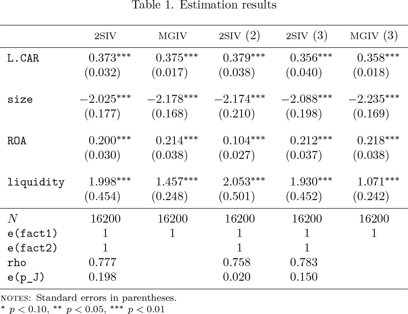
NOTES: Standard errors in parentheses.

^∗ p < 0.10, ^∗∗ p < 0.05, ^∗∗∗ p < 0.01

Columns 3–5 illustrate examples of IV estimators that allow for a more flexible specification of instruments than the baseline regression. In particular, column 3 shows results for a second-stage IV estimator that involves dropping ROA from the set of instruments and using an external variable instead, namely, ROE.¹⁵

The results in column 3 are similar to the baseline specification in column 1, except for the coefficient of ROA, which is statistically different at the 5% level. Note also that in this case the J-test statistic rejects the null hypothesis because the p-value equals 0.020. This implies that ROE may not form a valid instrument.

Column 4 corresponds to a second-stage IV estimator that we can compute by typing

In this specification, {size, ROA} are defactored based on a common set of factors estimated jointly, whereas liquidity is defactored separately, based on its own estimated factors. Such an instrumentation strategy can be particularly useful under three circumstances: first, when size and ROA are driven by entirely different factors than liquidity; second, when size and ROA have a different number of factors than liquidity; and third, when different lags of the covariates are used as instruments. Column 5 corresponds to the same specification as in column 4, although it refers to its MGIV version:

As we can see, the output of columns 4–5 is similar to that reported in columns 1–2, respectively. Therefore, the estimates appear to be fairly robust to different choices of instruments.

In terms of the notation used in the article, the choice of instruments corresponding to columns 4–5 is given by

{\hat{Z}}_{i} = (M_{{\hat{F}}_{x_{12}}} X_{i}^{(1, 2)}, M_{{\hat{F}}_{x_{12}, - 1}} X_{i, - 1}^{(1, 2)}, M_{{\hat{F}}_{x_{12}, - 2}} X_{i, - 2}^{(1, 2)}, M_{{\hat{F}}_{x_{3}}} X_{i}^{(3)}, M_{{\hat{F}}_{x_{3}, - 1}} X_{i, - 1}^{(3)})

where $X_{i}^{(1, 2)} = (X_{i}^{(1)}, X_{i}^{(2)}), {\hat{F}}_{x_{12}, - τ}$ is defined as $\sqrt{T}$ times the eigenvectors corresponding to the $m_{x}_{_{12}}$ largest eigenvalues of the T × T matrix $\sum_{i = 1}^{N} X_{i, - τ}^{(1, 2)} {(X_{i, - τ}^{(1, 2)})}^{'} / N T$ , and so on. The column dimension of the matrix of instruments is T × 8. Hence, two lags of $X_{i}^{(1, 2)}$ and one lag of $X_{i}^{(3)}$ are used as instruments. Note also that the maximum numbers of factors specified to be estimated from $X_{i}^{(1, 2)}$ and $X_{i}^{(3)}$ are different and equal 3 and 2, respectively.

Remark 7. For the MGIV estimator, although the matrix ${\hat{Z}}_{i}$ _i above is formulated by defactoring $X_{i}^{(1, 2)}$ and $X_{i}^{(3)}$ separately, the empirical projection matrix $M_{{\hat{F}}_{x}}$ used to defactor the entire model¹⁶ is computed by extracting factors jointly from the matrix of all covariates; that is, $X_{i} = (X_{i}^{(1)}, X_{i}^{(2)}, X_{i}^{(3)})$ .

In practice, users can avoid extracting factors jointly from the matrix of all covariates. For motivation, suppose that $X_{i}^{(3)}$ were a binary regressor that is not subject to a common factor structure. In that case, one may wish to 1) instrument $X_{i}^{(3)}$ by itself (that is, without defactoring or lags) and 2) defactor the entire model by extracting factors only from $X_{i}^{(1, 2)}$ , that is, to omit $X_{i}^{(3)}$ from the construction of $M_{{\hat{F}}_{x}}$ This can be achieved by specifying

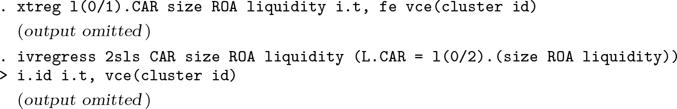
Defactoring of $X_{i}^{(3)}$ is avoided by specifying factmax(0). The omission of $X_{i}^{(3)}$ in the construction of $M_{{\hat{F}}_{x}}$ is achieved by specifying nodoubledefact. Note that in this case the number of estimated factors differs across covariates. Therefore, xtivdfreg reports Number of factors in X = * and provides detailed results on the estimated number of factors at the bottom of the output.

The columns in table 2 report results for several alternative popular estimators. To begin with, columns 1–2 correspond to the standard fixed-effects and 2SLS estimators, both of which accommodate a two-way error-components model, but they do not allow for common shocks:

Table 2.

Estimation results (continued)

	Fixed effect	2SLS	IV no DF	MGIV no DF	CCEP	CCEMG
L.CAR	0.878^∗∗∗ (0.018)	0.651^∗∗∗ (0.207)	0.651^∗∗∗ (0.207)	0.410^∗∗∗ (0.020)	0.526^∗∗∗ (0.039)	0.356^∗∗∗ (0.013)
size	−0.085^∗∗∗ (0.023)	−0.220^∗ (0.124)	−0.220^∗ (0.124)	−1.096^∗∗∗ (0.206)	−0.423^∗∗∗ (0.058)	−1.396^∗∗∗ (0.245)
ROA	0.101^∗ (0.055)	0.142(0.131)	0.142(0.131)	0.256^∗∗∗ (0.047)	0.130^∗∗ (0.056)	0.286^∗∗∗ (0.040)
liquidity	0.205(0.163)	0.503(0.460)	0.503(0.460)	1.581^∗∗∗ (0.283)	1.992^∗∗∗ (0.412)	1.740^∗∗∗ (0.253)
N	16500	16200	16200	16200	15900	15900
e(fact1)			0	0
e(fact2)
rho	0.061
e(p_J)			0.000

notes: Standard errors in parentheses.

^∗ p < 0.10, ^∗∗ p < 0.05, ^∗∗∗ p < 0.01

It is apparent that the estimated coefficients differ substantially compared with those obtained based on the 2SIV approach. In particular, the autoregressive coefficient appears to be biased upward, and—for the case of 2SLS (column 2)—the standard error of the estimate is much larger compared with the second-stage IV (see column 1 of table 1). On the other hand, the coefficients of ROA and liquidity seem to be biased in the opposite direction. Moreover, in three out of four cases, these coefficients are not statistically significant. This outcome is indicative of the importance of controlling for common shocks in the present example.

Column 3 reproduces the results of 2SLS using the xtivdfreg command. This is achieved by setting the number of factors equal to 0 and requesting the first-stage estimator:

Thus, the popular 2SLS estimator can be viewed as a special case of the 2SIV approach and arises by imposing zero number of factors (that is, setting factmax(0)) and fitting the model in a single stage (fstage). Column 4 yields 2SLS-type results for a model with heterogeneous slopes. Note that this option is not allowed in ivregress.

Finally, the last two columns correspond to the CCE estimator of Pesaran (2006). CCEP in column 5 denotes the pooled CCE estimator, and CCEMG in column 6 is the mean-group CCE version. These have been computed using the xtdcce2 command developed by Ditzen (2018).

As we can see, the estimates of CCEP are smaller than those obtained by the secondstage IV estimator (columns 1 and 4 of table 1), and the differences are statistically significant. On the other hand, the estimates of CCEMG are fairly close to those of the MGIV estimator in most cases. The main exception is the coefficient of size, which appears to be much smaller and less precise for CCEMG.

Remark 8. As pointed out by a referee, when the covariates are strictly exogenous, one can also use leads (as opposed to lags) as instruments. To see this, notice that the following two specifications are equivalent, provided that the number of estimated factors across all different lags of instruments is the same:

Hence, one can also use leads by typing

where F.() is the lead operator. Note that this equivalence does not hold when a second defactorization step is applied in stage one, that is, either for the model with heterogeneous slope coefficients or when the option doubledefact is declared:

To achieve equivalence in that case, exclude the lags or leads from the second defactorization, as follows:

4.2 Example 2: Estimation of cross-country production functions

To illustrate additional features of the xtivdfreg command for unbalanced panels, we use the macropanel dataset of Eberhardt and Teal (2010) for estimating cross-country production functions in the manufacturing sector. The dataset contains observations on 48 developing and developed countries during the period 1970 to 2002. These data are available as an ancillary file for the xtmg package, developed by Eberhardt (2012):

Following Eberhardt and Teal (2010), we focus on the following model, which imposes constant returns to scale:

\begin{matrix} In (\frac{Y_{i t}}{L_{i t}}) = β In (\frac{K_{i t}}{L_{i t}}) + u_{i t} \\ u_{i t} = η_{i} + τ_{t} + γ_{y i}^{'} f_{y, t} + ε_{i t} \end{matrix}

The dependent and independent variables denote the log value added per worker and the log capital stock per worker, respectively, for i = 1,…, 48, with each country observed over T_i observations.

We start by running the xtivdfreg command using two lags of the covariates as defactored instruments and up to a maximum of three factors. We use three instruments, and the degree of overidentification equals two. We control for bank-specific and timespecific effects by eliminating them prior to estimation. This baseline regression is computed by typing

Because the panel is unbalanced, the xtivdfreg command estimates the factors based on the iterative procedure described in section 2.3. The first line of dots reports the number of iterations required to estimate the factors in ln(K/L). The second (third) line of dots reports the number of iterations required to estimate the number of factors in the lagged (second lagged) value of ln(K/L). Finally, the last line corresponds to factor estimation from the first-stage residuals, which is relevant for the 2SIV estimator. In all cases, three iterations turn out to be sufficient for convergence.

The estimated coefficient of ln(K/L) is approximately equal to 0.5 and is statistically significant. The p-value of the J-test statistic indicates that the overidentifying restrictions are supported by the data. Moreover, ${\hat{m}}_{x}$ = ${\hat{m}}_{y}$ = 1, whereas the fraction of the variance of u_it that is explained by the factor component appears to be around 0.3.

Note that the number of lines of dots not only is a function of the number of lags used as instruments but also depends on whether factors are extracted jointly or individually for each regressor separately. For illustration, consider a similar model as in (13) but without imposing constant returns to scale:

In (Y_{i t}) = β_{1} In (L_{i t}) + β_{2} In (K_{i t}) + u_{i t}

We specify the iv() option twice, one for each individual regressor. This yields

This time, the number of dotted lines corresponding to factor estimation from the covariates has doubled. This is because the factors are extracted separately for ln (L) and ln (K), and therefore the algorithm performs twice the number of iteration loops.

MGIV estimation of the baseline regression in (13) is computed by typing

As we can see, the estimate of the coefficient of ln(K/L) is similar to that of the homogeneous model.¹⁷ For further analysis using this example, see Eberhardt and Teal (2010).

5 Conclusion

xtivdfreg is useful for estimating large panel-data models with unobserved common factors or interactive effects. The slope coefficients can be either homogeneous or heterogeneous. The command accommodates a flexible specification of instruments and incorporates the two-way error-components model as a special case. Results obtained from the popular ivregress command can be reproduced using xtivdfreg by imposing zero factors.

Supplemental Material

Supplemental Material, sj-zip-1-stj-10.1177_1536867X211045558 - Instrumental-variable estimation of large-T panel-data models with common factors

Supplemental Material, sj-zip-1-stj-10.1177_1536867X211045558 for Instrumental-variable estimation of large-T panel-data models with common factors by Sebastian Kripfganz and Vasilis Sarafidis in The Stata Journal

Footnotes

6 Acknowledgments

We are grateful to an anonymous referee for providing useful comments and suggestions. Vasilis Sarafidis gratefully acknowledges financial support from the Australian Research Council under research grant number DP-170103135.

7 Programs and supplemental materials

To install a snapshot of the corresponding software files as they existed at the time of publication of this article, type

To update the xtivdfreg package to the latest version, type

Notes

References

Ahn

S. C.

Horenstein

A. R.

2013. Eigenvalue ratio test for the number of factors. Econometrica 81: 1203–1227. https://doi.org/10.3982/ECTA8968.

Bai

2009. Panel data models with interactive fixed effects. Econometrica 77: 1229–1279. https://doi.org/10.3982/ECTA6135.

Bai

Liao

Yang

2015. Unbalanced panel data models with interactive effects. In The Oxford Handbook of Panel Data, ed. Baltagi

B. H.

, 149–170. Oxford: Oxford University Press. https://doi.org/10.1093/oxfordhb/9780199940042.013.0005.

Bai

2002. Determining the number of factors in approximate factor models. Econometrica 70: 191–221. https://doi.org/10.1111/1468-0262.00273.

Baltagi

B. H.

Wang

2021. Estimating and testing high dimensional factor models with multiple structural changes. Journal of Econometrics 220: 349–365. https://doi.org/10.1016/j.jeconom.2020.04.005.

Chudik

Pesaran

M. H.

2015. Large panel data models with cross-sectional dependence: A survey. In The Oxford Handbook Of Panel Data, ed. Baltagi

B. H.

, 3–45. Oxford: Oxford University Press. https://doi.org/10.1093/oxfordhb/9780199940042.013.0001.

Correia

2016. Estimating multi-way fixed effect models with reghdfe. Presented July 28–29, 2016, at the Stata Conference 2016, Chicago. https://www.stata.com/meeting/chicago16/slides/chicago16_correia.pdf.

Correia

2017. ftools: A faster Stata for large data sets. Presented July 27–28, 2017, at the Stata Conference 2017, Baltimore. https://www.stata.com/meeting/baltimore17/slides/Baltimore17_Correia.pdf.

Cui

Norkuté

Sarafidis

Yamagata

2020a. Two-stage instrumental variable estimation of linear panel data models with interactive effects. ISER Discussion Paper 1101, Institute of Social and Economic Research, Osaka University. https://ideas.repec.org/p/dpr/wpaper/1101.html.

10.

Cui

Sarafidis

Yamagata

2020b. IV estimation of spatial dynamic panels with interactive effects: Large sample theory and an application on bank attitude toward risk. Monash Business School, Working Paper 11 /20. https://doi.org/10.2139/ssrn.3642451.

11.

Ditzen

2018. Estimating dynamic common-correlated effects in Stata. Stata Journal 18: 585–617. https://doi.org/10.1177/1536867X1801800306.

12.

Eberhardt

2012. Estimating panel time-series models with heterogeneous slopes. Stata Journal 12: 61–71. https://doi.org/10.1177/1536867X1201200105.

13.

Eberhardt

Teal

2010. Productivity analysis in global manufacturing production. Discussion Paper 515, Department of Economics, University of Oxford. https://ora.ox.ac.uk/objects/uuid:ea831625-9014-40ec-abc5-516ecfbd2118.

14.

Harding

Lamarche

Pesaran

M. H.

2020. Common correlated effects estimation of heterogeneous dynamic panel quantile regression models. Journal of Applied Econometrics 35: 294–314. https://doi.org/10.1002/jae.2753.

15.

Jiang

Yang

Gao

Hsiao

Forthcoming. Recursive estimation in large panel data models: Theory and practice. Journal of Econometrics. https://doi.org/10.1016/j.jeconom.2020.07.055.

16.

Juodis

Karabiyik

Westerlund

2021. On the robustness of the pooled CCE estimator. Journal of Econometrics 220: 325–348. https://doi.org/10.1016/j.jeconom.2020.06.002.

17.

Juodis

Sarafidis

2018. Fixed T dynamic panel data estimators with multifactor errors. Econometric Reviews 37: 893–929. https://doi.org/10.1080/00927872.2016.1178875.

18.

Juodis

Sarafidis

Forthcoming. A linear estimator for factor-augmented fixed-T panels with endogenous regressors. Journal of Business & Economic Statistics . https://doi.org/10.1080/07350015.2020.1766469.

19.

Kapetanios

Serlenga

Shin

2021. Estimation and inference for multidimensional heterogeneous panel datasets with hierarchical multi-factor error structure. Journal of Econometrics 220: 504–531. https://doi.org/10.1016/j.jeconom.2020.04.011.

20.

Keeley

M. C.

1990. Deposit insurance, risk, and market power in banking. American Economic Review 80: 1183–1200.

21.

Kripfganz

Schwarz

2019. Estimation of linear dynamic panel data models with time-invariant regressors. Journal of Applied Econometrics 34: 526–546. https://doi.org/10.1002/jae.2681.

22.

Cui

2020. Efficient estimation of heterogeneous coefficients in panel data models with common shocks. Journal of Econometrics 216: 327–353. https://doi.org/10.1016/j.jeconom.2019.08.011.

23.

Martynova

Ratnovski

Vlahu

2020. Bank profitability, leverage constraints, and risk-taking. Journal of Financial Intermediation 44: 100821. https://doi.org/10.1016/j.jfi.2019.03.006.

24.

Moon

H. R.

Weidner

2015. Linear regression for panel with unknown number of factors as interactive fixed effects. Econometrica 83: 1543–1579. https://doi.org/10.3982/ECTA9382.

25.

Moon

H. R.

Weidner

2017. Dynamic linear panel regression models with interactive fixed effects. Econometric Theory 33: 158–195. https://doi.org/10.1017/S0266466615000328.

26.

Norkute

Sarafidis

Yamagata

Cui

2021. Instrumental variable estimation of dynamic linear panel data models with defactored regressors and a multifactor error structure. Journal of Econometrics 220: 416–446. https://doi.org/10.1016/j.jeconom.2020.04.008.

27.

Pesaran

M. H.

2006. Estimation and inference in large heterogeneous panels with a multifactor error structure. Econometrica 74: 967–1012. https://doi.org/10.1111/j.1468-0262.2006.00692.x.

28.

Sarafidis

Wansbeek

2012. Cross-sectional dependence in panel data analysis. Econometric Reviews 31: 483–531. https://doi.org/10.1080/07474938.2011.611458.

29.

Sarafidis

Wansbeek

2021. Celebrating 40 years of panel data analysis: Past, present and future. Journal of Econometrics 220: 215–226. https://doi.org/10.1016/j.jeconom.2020.06.001.

30.

Stock

J. H.

Watson

M. W.

1998. Diffusion indexes. NBER Working Paper No. 6702, The National Bureau of Economic Research. https://doi.org/10.3386/w6702.

31.

Jin

2012. Sieve estimation of panel data models with cross section dependence. Journal of Econometrics 169: 34–47. https://doi.org/10.1016/j.jeconom.2012.01.006.

32.

Westerlund

Urbain

J.-P.

2015. Cross-sectional averages versus principal components. Journal of Econometrics 185: 372–377. https://doi.org/10.1016/j.jeconom.2014.09.014.

Supplementary Material

Please find the following supplemental material available below.

For Open Access articles published under a Creative Commons License, all supplemental material carries the same license as the article it is associated with.

For non-Open Access articles published, all supplemental material carries a non-exclusive license, and permission requests for re-use of supplemental material or any part of supplemental material shall be sent directly to the copyright owner as specified in the copyright notice associated with the article.

0.33 MB

0.00 MB