Sage Journals: Discover world-class research

Abstract

We describe a new command, artcat, that calculates sample size or power for a randomized controlled trial or similar experiment with an ordered categorical outcome, where analysis is by the proportional-odds model. artcat implements the method of Whitehead (1993, Statistics in Medicine 12: 2257–2271). We also propose and implement a new method that 1) allows the user to specify a treatment effect that does not obey the proportional-odds assumption, 2) offers greater accuracy for large treatment effects, and 3) allows for noninferiority trials. We illustrate the command and explore the value of an ordered categorical outcome over a binary outcome in various settings. We show by simulation that the methods perform well and that the new method is more accurate than Whitehead’s method.

Keywords

st0700 artcat sample size power clinical trial randomized controlled trial noninferiority trial substantial-superiority trial categorical variable proportional-odds model evaluation

1 Introduction

The power of a randomized controlled trial or similar experiment is the probability that the primary analysis will show a statistically significant result in favor of the studied treatment (or other intervention). Designers of randomized controlled trials (which we henceforth simply call “trials”) typically aim to have 80% or 90% power for a given true treatment effect. Sample-size calculations are used to determine either the sample size required to give a specified power or the power implied by a specified sample size. Various formulas are in wide use (Julious 2009).

The most common sample-size calculation is for comparing two groups, treatment and control, also called “arms”. Multiarm trials improve efficiency by evaluating several new treatments in one trial (Parmar et al. 2017) and are usually designed using a two-group sample-size calculation, assuming that each treatment group will be compared with the control group. Sample-size calculations for general tests of heterogeneity between treatment groups are rarely used and are not discussed in this article.

In Stata, several standard sample-size calculations are available in the built-in power family. More advanced sample-size calculations are provided in the Analysis of Resources for Trials package (Barthel, Royston, and Babiker 2005; Barthel et al. 2006; Royston and Barthel 2010; Marley-Zagar et al. 2023).

However, none of these packages allows for an ordered categorical outcome, sometimes called an ordinal outcome. Such outcomes have been used, for example, in a trial evaluating treatments for influenza, where a six-category outcome was defined as 1) death, 2) in intensive care, 3) hospitalized but requiring supplemental oxygen, 4) hospitalized and not requiring supplemental oxygen, 5) discharged but unable to resume normal activities, or 6) discharged with full resumption of normal activities (Davey et al. 2019).

The present work was motivated by the need to consider the use of ordered categorical outcomes in a proposed trial of treatments for COVID-19, for example, a three-level outcome of death, in hospital, or alive and not in hospital. Other trials of treatments for COVID-19 have used various outcome scales, typically with six to eight ordered categories.

In this article, we introduce a new command, artcat, that addresses this need. The command performs sample-size calculations using the method of Whitehead (1993). We also introduce a new method that is both more flexible and more accurate than Whitehead’s method. The methods are described in section 5. The syntax is described in section 3.1, followed by examples in section 3, simulation evaluations in section 5, and a description of our procedures for testing the software in section 6. We end with section 7 suggesting future directions.

2 Methods

2.1 General sample-size formulas

Suppose the benefit of treatment is captured by an estimand θ (for example, a risk difference or log odds-ratio) so that the analysis of a superiority trial involves a significance test of the null hypothesis θ = 0. The designers of the trial want to ensure a high power, defined as the probability of a significant result, under the assumption that θ = d. Sample-size formulas relate the type II error (β = 1 − power) to the sample size n when the type I error is set to α. A general sample-size formula relates the required variance of an estimator $\hat{θ}$ to d, α, and β [Julious 2004, (2)],

var (\hat{θ}) = \frac{d^{2}}{{(z_{1 - α / 2} + z_{1 - β})}^{2}}

where z_p is the standard normal deviate with cumulative density p. Because var( $\hat{θ}$ ) is, to a very good approximation, inversely proportional to the total sample size n, we can write var( $\hat{θ}$ ) = V/n for some V : methods for calculating V in particular settings will be described below. Hence, the total sample-size requirement is

n = \frac{V {(z_{1 - α / 2} + z_{1 - β})}^{2}}{d^{2}}

The formula above implicitly assumes that the variance is the same under the null and alternative hypotheses, and this is not true for categorical outcomes. For example, for binary data, binomial variation follows distributions with different probabilities in the two groups, but under the null hypothesis, the average probability is assumed for both groups. We refine (1) by letting var( $\hat{θ}$ ) = V/n describe the variance of the estimator when θ = d, while var( $\hat{θ}$ ) = V _test/n describes its variance when the null hypothesis is assumed for the data. This gives an improved sample-size formula

n = \frac{{(\sqrt{V_{test}} z_{1 - α / 2} + \sqrt{V} z_{1 - β})}^{2}}{d^{2}}

Let var( $\hat{θ}$ ) = V_N /n under the null and V_A /n under the alternative hypothesis. A “local” test, assuming small treatment effects, sets V = V _test = V_N ; we call this method NN. A “distant” test, valid for small or large treatment effects, sets V = V_A . We may then have V _test = V_A (method AA), appropriate if a Wald test is used, or V _test = V_N (method NA), appropriate for the score test or approximations to it such as the likelihood-ratio test. All of these values are substituted into (2); methods NN and AA are given by the simpler formula (1) with V = V_N and V = V_A , respectively. This gives the formulas

Method NN: n = \frac{V_{N} {(z_{1 - α / 2} + z_{1 - β})}^{2}}{d^{2}}

Method NA: n = \frac{{(\sqrt{V_{N}} z_{1 - α / 2} + \sqrt{V_{A}} z_{1 - β})}^{2}}{d^{2}}

Method AA: n = \frac{V_{A} {(z_{1 - α / 2} + z_{1 - β})}^{2}}{d^{2}}

For binary data, these formulas are commonly used with the estimand θ defined as the risk difference. artbin offers a “local” method (NN), a “distant” method (NA), and a “Wald” method (AA). For ordinal data, θ will be defined as the log odds-ratio.

2.2 Whitehead’s method

We use the equations above in the specific case of an ordered categorical outcome Y and randomized treatment Z. Let the distribution of Y in the control group be p(Y = i|Z = c) = p_ci , and let the distribution of Y in the experimental (research) group be p(Y = i|Z = e) = p_ei , for i = 1,…, I. We initially assume for definiteness that outcome level 1 is the least favorable and level I is the most favorable and that the aim of the study is to demonstrate lower probabilities of the worse outcomes in the experimental group.

Whitehead (1993) considered the case where the n participants are randomized to control and experimental groups in the ratio a: 1 and the distributions of the outcome in the two groups obey a proportional-odds model,

logit \sum_{i = 1}^{i = k} p_{e i} = logit \sum_{i = 1}^{i = k} p_{c i} + θ

for any k = 1,…, I−1 (McCullagh 1980). Here θ is the log odds-ratio, which is assumed common across levels k. θ < 0 indicates lower probabilities of the less favorable outcomes in the experimental group and hence a beneficial treatment. This led to the formula

n = \frac{3 {(a + 1)}^{2} {(z_{1 - α / 2} + z_{1 - β})}^{2}}{a d^{2} (1 - \sum_{i} {\bar{p}}_{i}^{3})}

where ${\bar{p}}_{i} = (a p_{c i} + p_{e i}) / (a + 1)$ and d is the expected value of θ (Whitehead 1993).

This is a good and widely known formula. However, it has three limitations. First, it requires a common odds ratio to be specified at the design stage. In our experience, clinicians sometimes propose that treatments will reduce the risk of adverse outcomes by a fixed risk ratio so that p_ei /p_ci is the same for all i < I. This does not provide a value θ. Second, the expression used for the variance V is valid only under the null, so (7) represents method NN, and other methods may be more accurate; Whitehead (1993) discussed alternatives. Third, the formula does not cover noninferiority trials (see section 2.4 below). Our new proposal addresses these limitations.

2.3 New proposal

We propose a new method of sample-size determination that is valid for arbitrary sets of (p_ci, p_ei ) that may not obey the proportional-odds model. The idea is to evaluate V_N and V_A by constructing a dataset of expected outcomes and fitting the proportional-odds model with the ologit command.

We construct a dataset containing the expected outcomes per participant recruited. This contains two records for each outcome level: one for the experimental group and one for the control group. For each record, we compute the probability that a participant is randomized to that group and has his or her outcome at that level. For the control group, for outcome level i, this probability is p(Z = c)p(Y = i|Z = c) = ap_ci /(a + 1). For the experimental group, this probability is p(Z = e)p(Y = i|Z = e) = p_ei /(a + 1). These probabilities sum to 1.

We perform an ologit analysis of this dataset, using the weights as importance weights. This analysis yields the expected treatment effect d as the coefficient of Z. If the proportional-odds assumption does not hold, then d is interpreted as an average log odds-ratio. This analysis also yields the variance V_A as the estimated variance of the estimated coefficient of Z, so that the variance for a dataset of size n will be V_A /n. This is enough to implement method AA using (5).

For methods NN and NA, we change the weights to their values under the null, $a {\bar{p}}_{i} / (a + 1)$ and ${\bar{p}}_{i} / (a + 1)$ , and refit the ologit analysis. Then V_N is the estimated variance of the estimated coefficient of Z. We can then use (3) for method NN and (4) for method NA.

2.4 Noninferiority trials

In a noninferiority trial, the null hypothesis is that the experimental treatment is worse than the control treatment by a prespecified amount m, termed the margin. The margin typically represents a small degree of worsening of the primary outcome that is judged to be acceptable because of other advantages of the experimental treatment that are not captured by the primary outcome. In the setting of a categorical outcome ordered from least (1) to most (I) favorable outcome, the margin is expressed as an odds ratio greater than 1, and m > 0 is the log odds-ratio. The null hypothesis is then θ = m, and the alternative hypothesis is θ < m. Typically, the investigators expect the true treatment effect to be 0, so that p_ei = p_ci for all i and d = 0, but some noninferiority trials are designed under the expectation that the experimental treatment is somewhat beneficial and so d < 0 (for example, Nunn et al. [2019]).

The expected (alternative) variance of the estimate is given in the same way as for a superiority trial, but the test (null) variance must be calculated differently to reflect the noninferiority null. This is easily done in the ologit framework described above, with (2) modified to

n = \frac{{(\sqrt{V_{test}} z_{1 - α / 2} + \sqrt{V} z_{1 - β})}^{2}}{{(d - m)}^{2}}

Steps 1 and 2 are unchanged. At step 3, we fit model (6) to the dataset of expected results per participant under the null θ = m by using the offset() option of ologit. We then estimate the fitted probabilities, with which we revise the dataset of expected results per participant and fit model (6) again, yielding the test (null) variance V_N . If this procedure is applied with m = 0, then the results are the same as with a superiority trial.

These methods also apply without modification to a substantial-superiority trial, in which the aim is to show that the experimental treatment is substantially superior to the control; this is implemented by setting the margin m < 0. A substantial-superiority trial requires a larger sample size than a superiority trial with the same expected treatment effect.

2.5 Risk difference, risk ratio, or odds ratio

The odds ratio is often a sensible estimand for an ordered categorical outcome because it is plausibly constant across different levels [k in (6)], unlike the risk difference and risk ratio. For a binary outcome, this issue does not arise, and the risk difference or risk ratio is usually preferred because of its simpler interpretation (Altman, Deeks, and Sackett 1998).

In the binary outcome case, we may ask how sample-size calculations with the different estimands compare. In a superiority trial, all estimands imply the same null hypothesis—that the two treatments are equal. Sample-size calculations with different estimands then address the same question but use different approximations: artbin assumes a normal distribution for the estimated risk difference, while artcat assumes this for the estimated log odds-ratio. We will explore the impact of these different approximations in section 4.2. In a noninferiority trial, by contrast, the null hypothesis depends on the estimand used (Quartagno et al. 2020), so sample-size calculations with different estimands are not comparable and may differ markedly.

3 Syntax

artcat, pc( numlist ) {pe( numlist )| or( exp )| rr( exp )} [[ power( # )| n( # )] cumulative [ unfavourable| unfavorable| favourable| favorable] margin( # ) aratio( # # ) alpha( # ) onesided ologit[( type )] whitehead noprobtable probformat( string ) format( string ) noround noheader]

3.1 Options

pc( numlist ) specifies the probabilities in each outcome level; the rightmost level may be omitted. pc() is required.

pe( numlist ) specifies the probabilities in each outcome level, specified as for pc(); or cumulative probabilities, if the cumulative option is used. One of pe(), or(), or rr() must be specified.

or( exp ) specifies the odds ratio at each outcome level. An odds ratio less than 1 means that the distribution in the experimental group is shifted toward the rightmost level compared with the control group. One of pe(), or(), or rr() must be specified.

rr( exp ) specifies the risk ratio at each outcome level except the rightmost. A risk ratio less than 1 means that the experimental group has lower probability at every level except the rightmost level compared with the control group. One of pe(), or(), or rr() must be specified.

power( # ) specifies the power required; sample size will be computed. The default is power(0.8) if neither power() nor n() is specified. You cannot specify both power() and n().

n( # ) specifies the total sample size; power will be computed. You cannot specify both power() and n().

cumulative specifies that the probabilities in pc() are cumulative probabilities.

unfavourable or unfavorable specifies that the leftmost outcome level represents the least favorable outcome. Both American and English spellings are allowed.

favourable or favorable specifies that the leftmost outcome level represents the most favorable outcome. Both American and English spellings are allowed.

margin( # ) specifies the margin, as an odds ratio, for a noninferiority or a substantialsuperiority trial. If the unfavorable option is specified, then # > 1 specifies a noninferiority trial, and # < 1 specifies a substantial-superiority trial. If the favorable option is specified, then it is the other way around. If margin() is not specified or if margin(1) is specified, then a superiority trial is assumed.

aratio( # # ) specifies the allocation ratio; for example, aratio(1 2) means 2 participants in the experimental group for every 1 participant in the control group.

alpha( # ) specifies the significance level. The default is alpha(0.05).

onesided specifies that the level specified by alpha() is the one-sided significance level. The default is a two-sided significance level.

ologit[( type )] uses the ologit (new) method. type may be NN, NA, or AA. The default is ologit(NA). ologit is the same as ologit(NA).

whitehead uses the Whitehead method. This option requires or() to be specified and is not available with margin().

noprobtable specifies not to display the table of anticipated probabilities (probabilities at each level in the control and experimental groups).

probformat( string ) specifies the format for displaying table of anticipated probabilities. The default is probformat(%-5.1f).

format( string ) specifies the format for displaying calculated sample sizes (default is format(%6.1f)) or powers (default is format(%6.3f)).

noround specifies not to round the sample size per group to the next largest integer.

noheader specifies not to print the header describing the program.

3.2 Favorable and unfavorable outcomes

The user is recommended to specify whether the leftmost levels of the outcome are favorable or unfavorable. However, the program also works this out for itself. In a superiority trial, an expected odds ratio smaller (larger) than 1 implies an unfavorable (favorable) outcome. If the margin is specified, then the criterion is whether the expected odds ratio is smaller or larger than the margin. If the user has specified the favorable or unfavorable option, then this is checked; if not, the program prints a note stating which it has inferred.

4 Examples

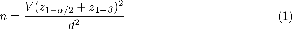
4.1 Six-level outcome

We reproduce the sample-size calculation for the FLU-IVIG trial (Davey et al. 2019). The control arm is expected to have a 1.8% probability of the least favorable outcome (death), a 3.6% probability of the next worst outcome (admission to an intensive care unit), and so on. The trial is designed to have 80% power if the treatment achieves an odds ratio of 1.77 for a favorable outcome. We invert this to match the assumption above of an unfavorable outcome.

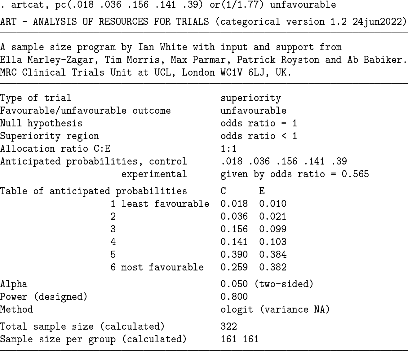
A total sample size of 322 participants (in both trial arms combined) is required. Below, we get the same answer by reversing the order of levels and hence focusing on favorable outcomes. The last probability could be omitted in the syntax. We use the noheader option to shorten the output. Note that the probabilities at each level in each arm agree with the previous output.

We can also check the power if we recruit 322 participants; in principle, we expect this to be exactly 80%, but because the sample size above is rounded to the next largest integer, the power is slightly more than 80%. We use the noprobtable option to suppress the table of assumed probabilities.

We next compare the new methods with the Whitehead method.

The Whitehead method gives a sample size just 2 less than the ologit(NA) method. Using the ologit(NN) option would show that the new method NN agrees exactly with the Whitehead method.

Suppose that the FLU-IVIG trial found that the experimental treatment worked exactly as proposed and that a further noninferiority trial is designed to show that a second new treatment has an odds ratio no worse than 1.33 compared with the first new treatment. We can design this trial using

The noninferiority trial requires a sample size of 1,314.

4.2 Binary outcome and comparison with artbin

artcat handles the case of a binary outcome, so we compare it with the standard sample-size calculations performed by artbin for a binary outcome with probability 0.4 on control and 0.2 on experimental treatment.

artbin gives a sample size just 2 greater than artcat. As noted in section 2.5, this is because the two procedures answer the same question but use different approximations.

4.3 Effect of subdividing the categories

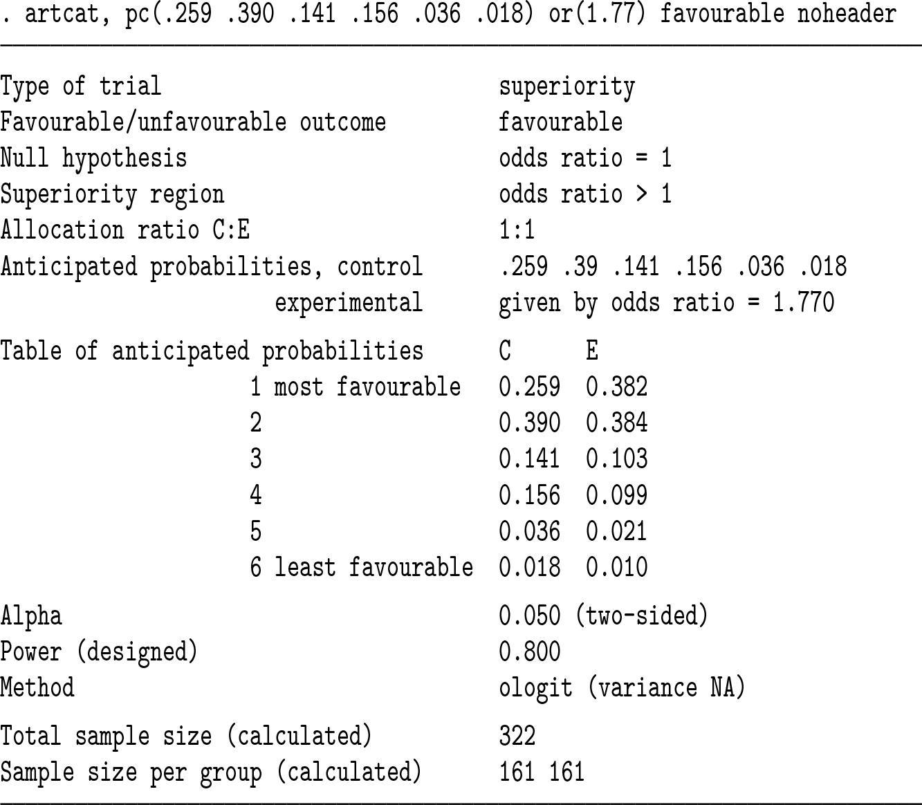
We finally explore the value of subdividing the unfavorable outcome level of section 4.2, assuming a common odds ratio of (0.2/0.8)/(0.4/0.6) = 0.375 at all levels. We first add an outcome level of control probability 0.01 and then another of control probability 0.09.

We see that adding an outcome level of low prevalence has a negligible effect on sample size. The biggest gains in sample size are achieved when a large outcome level is split, for example, if the healthy category with control probability 0.6 can be subdivided:

However, in practice, subdividing a healthy category may mean that the most important clinical differences are swamped by less important differences, which is a concern if the proportional-odds assumption may not hold. For example, suppose category 1 is death or disability, category 2 is hospitalization and healthy discharge, and category 3 is healthy without hospitalization. If treatment reduces the risk of hospitalization but not the risk of death or disability, then the treatment may be estimated to be beneficial, and it may therefore wrongly be seen as preventing death or disability.

5 Evaluations

5.1 Evaluation 1: Six-level outcome based on the FLU-IVIG study

We explore the difference between methods for the FLU-IVIG setting across a range of odds ratios. Data are assumed to follow the control outcome distribution as proposed, and the common odds ratio is fixed at values from 0.2 to 0.8. Sample sizes to give 90% power, estimated by the different methods, are shown in table 1. Differences are consistently about 10. The relative difference between methods is therefore greater at more extreme odds ratios.

Table 1.

Sample sizes required to give 90% power for the FLU-IVIG setting, estimated by the Whitehead and new sample-size formulas

Odds	Sample size for 90% power
ratio	Whitehead	New NN	New NA	New AA
0.2	56	56	60	67
0.3	98	98	102	109
0.4	168	168	172	178
0.5	291	291	295	302
0.6	534	534	538	544
0.7	1090	1090	1094	1101
0.8	2777	2777	2781	2787

We next evaluate the methods by simulation to gauge the accuracy of the estimated powers. We simulate data assuming that exactly half the sample is assigned to each group, using the FLU-IVIG control outcome distribution and a common odds ratio fixed at values from 0.2 to 0.8. The sample size is determined from the same parameters by the Whitehead method to give 90% power. We test the null hypothesis of no treatment effect using a Wald test in the ologit model. The power is the proportion of repetitions in which the null hypothesis is rejected and is compared with power estimated by each of the methods described in the earlier sections. We use 100,000 repetitions to get very small Monte Carlo errors (Morris, White, and Crowther 2019).

Results (table 2) show moderate differences between methods at extreme odds ratios and negligible differences at large odds ratios. Simulation results are closest to those for the “new NA” method, which is slightly conservative (that is, it slightly underestimates power). The Whitehead and “new NN” methods are anticonservative, and the “new AA” method is conservative and the least accurate.

Table 2.

Power for the FLU-IVIG setting, estimated by the Whitehead and new samplesize formulas and by simulation. Sample sizes are chosen to give 90% power under the Whitehead method. Monte Carlo standard error in the simulation results is 0.1%.

Odds	Sample	Power % from sample-size formula or simulation
ratio	size	Whitehead	New NN	New NA	New AA	Simulation
0.2	56	90.1	90.1	88.1	84.5	88.4
0.3	98	90.1	90.1	88.9	86.9	89.2
0.4	168	90.1	90.1	89.4	88.3	89.5
0.5	291	90.0	90.0	89.6	89.0	89.6
0.6	534	90.0	90.0	89.8	89.5	89.7
0.7	1090	90.0	90.0	89.9	89.7	90.1
0.8	2777	90.0	90.0	90.0	89.9	90.1

5.2 Evaluation 2: Two levels

We compare artcat with the standard sample-size calculations performed by power and artbin for a two-level outcome. We set p_c ₁ = 0.2 or 0.02 and vary the odds ratio due to treatment from 0.2 to 0.8. To estimate sample size with artbin, we use both the method that assumes local alternatives (variance type NN) and the method that allows distant alternatives (variance type NA); and with artcat, we use the Whitehead and new NN, NA, and AA alternatives. Variance types are not comparable between artbin and artcat, because they work on different scales. In particular, artbin works on the risk difference scale, so local (NN) is most conservative, while artcat works on the log odds-ratio scale, so AA is most conservative. The results in table 3 show that artbin and power perform very similarly in all cases, and all methods perform very similarly for odds ratios of 0.7 or 0.8. Differences between artcat methods and between artcat and artbin become more pronounced as odds ratios become more extreme. Again, the NA method of artcat is closest to artbin, but it gives sample sizes more than 10% smaller than artbin when p_C = 0.2 and odds ratio = 0.2 or when p_C = 0.02 and odds ratio = 0.2 or 0.3.

Table 3.

Sample sizes required to give 90% power for an unfavorable outcome, estimated by power, artbin, and the Whitehead and new methods

Control	Odds	Sample size
fraction	ratio	power	artbin		artcat
p_c ₁			local	distant	Whitehead	New NN	New NA	New AA
0.20	0.2	194	197	192	150	150	180	230
0.20	0.3	286	290	285	249	249	274	314
0.20	0.4	436	439	436	403	403	425	460
0.20	0.5	696	699	694	666	666	686	717
0.20	0.6	1194	1198	1198	1168	1168	1186	1214
0.20	0.7	2318	2322	2322	2294	2294	2311	2336
0.20	0.8	5660	5664	5664	5638	5638	5654	5677
0.02	0.2	1964	1968	1968	1365	1365	1746	2418
0.02	0.3	2792	2795	2795	2253	2253	2585	3137
0.02	0.4	4106	4110	4110	3615	3615	3914	4394
0.02	0.5	6356	6359	6359	5902	5902	6176	6607
0.02	0.6	10622	10626	10626	10201	10201	10454	10848
0.02	0.7	20118	20121	20121	19722	19722	19959	20324
0.02	0.8	48042	48045	48045	47670	47670	47893	48235

Given the differences between the methods shown in table 3, we use simulation to evaluate the methods in this setting. We fix p_c = 0.2 and use the same range of odds ratios. We fix the sample size for each odds ratio at that chosen to give 90% power by artbin with default options. The Whitehead method is omitted because, as seen above, it is the same as the new NN method, and power is omitted because it agrees closely with artbin. We test the null hypothesis of no treatment effect using a Wald test in the logit model. Some simulated datasets with odds ratio = 0.2 or 0.3 have perfect prediction because no events occur in the experimental group: analysis of such datasets using logit yields a standard error of zero and a missing Wald test result. Therefore, we also use a Pearson’s χ ² test. The power is the proportion of repetitions in which the null hypothesis is rejected and is compared with power estimated by each of the methods described in the earlier sections. The asymptotic properties of the Wald and Pearson tests may not hold in the smaller sample sizes, and hence we also evaluate the type I error of each test by repeating the simulation with the same sample sizes but with the odds ratio changed to 1. We again use 100,000 repetitions.

The results (table 4) show that all methods perform accurately for odds ratios of 0.7 or 0.8; that is, their estimated powers are very close to those found by simulation. For smaller (more extreme) odds ratios, new methods NN and AA are inaccurate, respectively overestimating and underestimating power. artbin underestimates power by up to 3%, and new method NA appears to be the most accurate, with slight underestimation of power (by less than 1%) compared with simulated power using the Pearson test. Type I error is close to the nominal 5%, suggesting that the simulated powers are accurate.

Table 4.

Power with an unfavorable binary outcome, estimated by artbin, artcat, and simulation. The control group proportion is fixed at 0.2. Sample sizes are chosen to give 90% power by artbin with distant option. The Monte Carlo standard error in the simulation results is 0.1%.

Odds	Sample	Power % by given method							Type I
ratio	size	artbin		artcat new			Simulation		error %
		local	distant	NN	NA	AA	Wald	Pearson	Wald	Pearson
0.2	192	89.4	90.0	95.7	91.7	84.2	90.6	92.1	4.6	5.1
0.3	285	89.6	90.0	93.5	91.1	87.0	90.9	91.3	4.9	5.0
0.4	436	89.8	90.1	92.1	90.7	88.5	90.2	90.7	4.9	5.0
0.5	694	89.8	90.0	91.1	90.3	89.1	90.1	90.4	5.0	5.0
0.6	1198	90.0	90.1	90.7	90.3	89.6	90.3	90.3	4.9	4.9
0.7	2322	90.0	90.1	90.3	90.1	89.8	90.2	90.2	5.0	5.0
0.8	5664	90.0	90.0	90.1	90.1	89.9	90.0	90.0	5.0	5.0

In sensitivity analysis, we varied p_c ₁ to 0.1 and 0.4, and results (not shown) showed similar patterns.

6 Software testing

This software is for use in the design of randomized trials, so we have been careful to test it extensively. The program was written by Ian R. White and tested by Ella Marley-Zagar. Here we report these testing methods.

We compared results with those given by Whitehead (1993). Exact agreement was achieved.

We compared results for a binary outcome in a superiority trial with those given by artbin and power across a range of probabilities and allocation ratios. Close, but not exact, agreement was achieved, except in a few well-understood cases.

We checked error messages in several impossible cases, for example, a negative odds ratio.

We compared results with those given by the R package dani (Quartagno 2020). This calculates sample sizes for a binary outcome on the odds-ratio scale for noninferiority trials and implicitly uses the AA method. Exact agreement was achieved for the AA method.

We reran the test scripts, implementing the above tests in Stata 13 and 16, with the default variable types (set type) as float and double.

We did various tests of internal consistency of the program. We compared different ways of stating the same problem (for example, interchanging C and E groups or reversing the order of the categories) and verified that the same answer was achieved. We calculated the power p for a sample size n, calculated the sample size for power p, then checked that this equaled the original n. We changed options that should change the sample size and verified that they did change the sample size.

The simulations reported in section 5 also test the software.

7 Conclusions

We have provided software to facilitate sample size and power calculation using Whitehead’s method and also proposed a new method, the ologit method with NA variance. We have shown that Whitehead’s method can be anticonservative (underestimates sample size and overestimates power), while the new NA method is accurate.

Surprisingly, we have also shown for a binary outcome that the new NA method may outperform the standard method implemented in artbin and power, with the standard method being slightly conservative for very large treatment effects. This may be because the new NA method makes a normal approximation on the log odds scale, while the artbin method makes a normal approximation on the probability scale, and the former may be a better approximation. However, the differences between the methods are small, apply only in the unrealistic setting of huge treatment effects, and should not discourage the use of artbin or power.

artcat can also be used to design observational studies to explore a protective or harmful factor in the absence of substantial confounding. The trial types and outcome levels may need to be reinterpreted as shown in the help file. For example, an observational study design to demonstrate a protective factor could be designed in exactly the same way as a trial, but the term “superiority” might be replaced by “benefit”.

A useful future extension will be to allow covariate adjustment, and this can be straightforwardly implemented using the ologit method. Another future extension could be to allow more than two groups, as artbin does. The idea of analyzing an expected dataset may be useful in other sample-size calculations.

9 Programs and supplemental materials

Supplemental Material, sj-zip-1-stj-10.1177_1536867X231161934 - artcat: Sample-size calculation for an ordered categorical outcome

Supplemental Material, sj-zip-1-stj-10.1177_1536867X231161934 for artcat: Sample-size calculation for an ordered categorical outcome by Ian R. White, Ella Marley-Zagar, Tim P. Morris, Mahesh K. B. Parmar, Patrick Royston and Abdel G. Babiker in The Stata Journal

Footnotes

8 Acknowledgments

This work was supported by the Medical Research Council Unit Programme numbers MC_UU_12023/29 and MC_UU_00004/09. We thank Clifford Silver Tamaro and Oliva Safari for help in testing the program.

9 Programs and supplemental materials

To install a snapshot of the corresponding software files as they existed at the time of publication of this article, type

You can get the latest version of artcat using

The code we used for testing and the testing results are included in the package. The GitHub repository includes these and also contains the latest version of the program and the code for the evaluations in section 5.

References

Altman

D. G.

Deeks

J. J.

Sackett

D. L.

. 1998. Odds ratios should be avoided when events are common. BMJ 317: 1318. https://doi.org/10.1136/bmj.317.7168.1318.

Barthel

F. M.-S.

Babiker

Royston

Parmar

M. K. B.

. 2006. Evaluation of sample size and power for multi-arm survival trials allowing for non-uniform accrual, non-proportional hazards, loss to follow-up and cross-over. Statistics in Medicine 25: 2521–2542. https://doi.org/10.1002/sim.2517.

Barthel

F. M.-S.

Royston

Babiker

. 2005. A menu-driven facility for complex sample size calculation in randomized controlled trials with a survival or a binary outcome: Update. Stata Journal 5: 123–129. https://doi.org/10.1177/1536867X0500500114.

Davey

R. T.

Fernández-Cruz

Markowitz

Pett

Babiker

A. G.

Wentworth

Khurana

, et al. 2019. Anti-influenza hyperimmune intravenous immunoglobulin for adults with influenza A or B infection (FLU-IVIG): A double-blind, randomised, placebo-controlled trial. Lancet Respiratory Medicine 7: 951–963. https://doi.org/10.1016/S2213-2600(19)30253-X.

Julious

S. A.

2004. Sample sizes for clinical trials with Normal data. Statistics in Medicine 23: 1921–1986. https://doi.org/10.1002/sim.1783.

Julious

S. A.

2009. Sample Sizes for Clinical Trials. Boca Raton, FL: Chapman & Hall/CRC

Marley-Zagar

White

I. R.

Royston

Barthel

F. M.-S.

Parmar

M. K. B.

Babiker

A. G.

2023. artbin: Extended sample size for randomised trials with binary outcomes. Stata Journal 23: 24–52. https://doi.org/10.1177/1536867X231161971.

McCullagh

1980. Regression models for ordinal data. Journal of the Royal Statistical Society, Series B 42: 109–142. https://doi.org/10.1111/j.2517-6161.1980.tb01109.x.

Morris

T. P.

White

I. R.

Crowther

M. J.

. 2019. Using simulation studies to evaluate statistical methods. Statistics in Medicine 38: 2074–2102. https://doi.org/10.1002/sim.8086.

10.

Nunn

A. J.

Phillips

P. P. J.

Meredith

S. K.

Chiang

C.-Y.

Conradie

Dalai

van Deun

, et al. 2019. A trial of a shorter regimen for rifampin-resistant tuberculosis. New England Journal of Medicine 380: 1201–1213. https://doi.org/10.1056/NEJMoa1811867.

11.

Parmar

M. K. B.

Sydes

M. R.

Cafferty

F. H.

Choodari-Oskooei

Langley

R. E.

Brown

Phillips

P. P. J.

, et al. 2017. Testing many treatments within a single protocol over 10 years at MRC Clinical Trials Unit at UCL: Multi-arm, multi-stage platform, umbrella and basket protocols. Clinical Trials 14: 451–461. http://doi.org/10.1177/1740774517725697.

12.

Quartagno

. 2020. dani: Design and analysis of non-inferiority trials. R package version 0.1 -1. https://cran.r-project.org/package=dani.

13.

Quartagno

Walker

A. S.

Babiker

A. G.

Turner

R. M.

Parmar

M. K. B.

Copas

White

I. R.

. 2020. Handling an uncertain control group event risk in noninferiority trials: Non-inferiority frontiers and the power-stabilising transformation. Trials 21: 145. https://doi.org/10.1186/s13063-020-4070-4.

14.

Royston

Barthel

F. M.-S.

. 2010. Projection of power and events in clinical trials with a time-to-event outcome. Stata Journal 10: 386–394. https://doi.org/10.1177/1536867X1001000306.

15.

Whitehead

1993. Sample size calculations for ordered categorical data. Statistics in Medicine 12: 2257–2271. https://doi.org/10.1002/sim.4780122404.

Supplementary Material

Please find the following supplemental material available below.

For Open Access articles published under a Creative Commons License, all supplemental material carries the same license as the article it is associated with.

For non-Open Access articles published, all supplemental material carries a non-exclusive license, and permission requests for re-use of supplemental material or any part of supplemental material shall be sent directly to the copyright owner as specified in the copyright notice associated with the article.

0.00 MB