Sage Journals: Discover world-class research

Abstract

The sample size of a randomized controlled trial is typically chosen in order for frequentist operational characteristics to be retained. For normally distributed outcomes, an assumption for the variance needs to be made which is usually based on limited prior information. Especially in the case of small populations, the prior information might consist of only one small pilot study. A Bayesian approach formalizes the aggregation of prior information on the variance with newly collected data. The uncertainty surrounding prior estimates can be appropriately modelled by means of prior distributions. Furthermore, within the Bayesian paradigm, quantities such as the probability of a conclusive trial are directly calculated. However, if the postulated prior is not in accordance with the true variance, such calculations are not trustworthy. In this work we adapt previously suggested methodology to facilitate sample size re-estimation. In addition, we suggest the employment of power priors in order for operational characteristics to be controlled.

Keywords

Sample size re-estimation power prior Bayesian randomized controlled trial monitoring variance borrowing

1 Introduction

A frequentist approach is typically employed for the design and analysis of a randomized controlled trial (RCT). The sample size is thus chosen in order for frequentist operational characteristics to be retained. This is done by specifying the power (1 − β) with which to detect a clinically relevant treatment effect (δ^*), given a type I error (α). For an RCT with two groups of equal size being compared on a normally distributed outcome with common unknown variance (σ²), δ is commonly measured as the difference between the two groups’ means. If we are interested in testing H₀: δ = 0 versus H₁: δ > 0 with δ^*> 0, the sample size is determined by finding the first even integer solution to satisfy the following inequality

N \geq 4 σ_{0}^{2} (\frac{t_{N - 2, 1 - α} + t_{N - 2, 1 - β}}{δ^{*}})^{2}

(1)

where N represents the required sample size,

t_{N - 2, 1 - α}

represents the (1 − α) point of the t-distribution with N − 2 degrees of freedom, and

σ_{0}^{2}

represents an initial assumption for the variance.

The assumption for the variance is usually based on limited prior information. Especially in the case of small or sensitive populations such as the ones defined by rare diseases or pediatric patients, the prior information might consist of only one small pilot study. Calculating the sample size can therefore be subject to considerable uncertainty.¹ Overestimation of the variance can result in committing to more resources than necessary, while underestimation can lead to inconclusive results. Both situations are undesirable when available research participants are limited.

A vast amount of methods have been developed to deal with such situations.^2–5 These methods have in common that they monitor the interim estimates of parameters within a trial, and respond to these estimates by re-calculating the required sample size to meet the design characteristics. Methods that only monitor nuisance parameters, such as the variance, are generally well accepted, but methods responding to interim estimates of the treatment effect can introduce bias.⁶ However, in the frequentist framework, quantification of the uncertainty about the estimate of the variance remains an obstacle. The variability of this (interim) estimate is dependent on the amount of data collected and is substantial if only a small amount of subjects have been recruited.⁷ In addition, if the variance is monitored only once, its estimator will be negatively biased by the end of the trial.¹ This is because an underestimation of the true variance at interim causes the required sample size to be re-estimated downwards. It is thus increasingly difficult to correct this erroneous estimate in the remaining sample size.² On the other hand, when the true variance is overestimated at interim, the sample size is re-estimated upwards, allowing enough time to adjust the estimate by the end of the trial. Friede and Miller¹ suggest continuous monitoring and re-estimation as a preferred solution for these issues. However, continually altering the original design based on an unstable estimate can come at great costs. Repeated sample size re-estimation (SSR) limits the amount of times the sample size can be re-estimated,¹ but still fails to clearly recommend when it is appropriate to do so. This is especially important when dealing with RCTs with a small available study population.

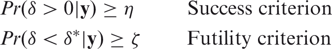
A Bayesian approach formalizes the aggregation of prior information on the variance with newly collected data, potentially alleviating some of the issues mentioned above.⁸ Calculating the sample size necessary for a Bayesian RCT depends on the decision scheme that is to be followed after completion of the trial. Several different methods have been proposed, including hybrid frequentist-Bayesian,^9–12 fully decision theoretic^13–16 and interval-length based approaches.^17–19 Whitehead et al.⁸ have advocated a variant of the latter which is comparable in simplicity to the frequentist sample size calculation (equation (1)) and includes an analogy to frequentist type I and II errors. This design requires the formulation of two hypotheses: (1) δ > 0, indicating that the experimental group performs better than the control, and (2) δ < δ^*, concluding that the experimental treatment fails to improve upon control by a defined clinically relevant difference.⁸ The sample size needs to be large enough to provide convincing evidence that either (1) or (2) is the case. Even though the same notation is used for δ^* to point out the similarity in this approach and the standard frequentist one, the two effect sizes are not necessarily equivalent conceptually.

When the variance is unknown, the sample size is calculated using a belief about the variance in the form of a prior distribution. If this belief is in agreement with the actual data-generating mechanism, the calculated sample size ensures that the design characteristics will be fulfilled by the end of the trial. If this is not the case, recruiting the original sample size might not be enough to satisfy either of the hypotheses, leading to an inconclusive trial. Just as in the frequentist context, monitoring the variance during the trial can facilitate interim SSR. Several approaches have been proposed using external information for sample size adjustment in a Bayesian framework.^20–23 In particular, Zhong et al.²⁴ discuss SSR for RCTs with a binary outcome, but a similar approach has not been considered for RCTs with a continuous outcome.

Moreover, when there is conflict between the prior and the data, Bayesian procedures can have unpredictable, and likely undesirable, frequentist characteristics. The power prior approach²⁵ can be employed in order to discard the influence of prior information on posterior inference; this is achieved by employing a power parameter $γ \in [0, 1]$ which usually translates as a deflating factor of the precision of the prior distribution. The application of power priors in sample size determination has been considered before.²⁶ The most challenging aspect in employing power priors is the specification of γ. Adaptive formulations of the power prior^27–29 allow for γ to be estimated based on the similarity between the prior and current data and thus, with appropriate calibration, achieve desired operational characteristics.

In light of the above, the goal of the present research is to explore the operational characteristics of the sample size determination method proposed inWhitehead et al.⁸ in the case of misspecified variance and to demonstrate the effects of SSR by interim variance monitoring. We employ the power prior approach introduced in Nikolakopoulos et al.²⁹ to synthesize prior and new data in order for operational characteristics (in this case the probability of having a conclusive trial) to be calibrated.

The paper is organized as follows: in the following section, the sample size determination procedure described in Whitehead et al.⁸ is outlined and adapted to allow for SSR. The adaptive power prior, based on predictive distributions and termed Prior-Data conflict calibrating power prior (PDCCPP) in Nikolakopoulos et al.,²⁹ is then briefly described and applied in the variance re-estimation problem. Subsequently, the proposed approach is demonstrated for a clinical trial in the field of pediatrics. The paper ends with a discussion.

2 Bayesian sample size determination

We consider the case where an RCT is designed to evaluate an experimental treatment (E) against a control (C) on a normally distributed outcome ( $Y_{j} \sim N (μ_{j}, σ^{2})$ , where j = E, C) with unknown variance (σ²). Y_ji is the outcome value of subject i in group j. In the Bayesian framework the precision (ν = 1/σ²) is often used for modeling purposes. The required sample size is denoted by N, where N = N_E + N_C. A positive value for δ = μ_E − μ_C indicates that E is better than C. A gamma prior distribution is assumed for ν with parameters α₀ and β₀. This corresponds to 2α₀ observations with a sample precision of α₀/β₀. The conditional prior for μ_j, given ν, is normal with mean μ₀ _j and precision $q_{0 j} ν$ . This information corresponds to q₀ _j virtual patients with an average of μ₀ _j on the outcome variable.³⁰ The posterior of μ_j, given ν, is also normal with mean μ₁ _j and precision $q_{1 j} ν$ , where $μ_{1 j} = μ_{0 j} (q_{0 j} / q_{1 j}) + N_{j} {\bar{y}}_{j} / q_{1 j}$ and $q_{1 j} = q_{0 j} + N_{j}$ . ν has a gamma posterior distribution with $α_{1} = α_{0} + \frac{N}{2}$ and $β_{1} = β_{0} + \frac{H}{2}$ where

H = \sum_{i = 1}^{N_{E}} (y_{Ei} - {\bar{y}}_{E})^{2} + \sum_{i = 1}^{N_{C}} (y_{Ci} - {\bar{y}}_{C})^{2} + \frac{N_{C} q_{0 C} ({\bar{y}}_{C} - μ_{0 C})^{2}}{q_{0 C} + N_{C}} + \frac{N_{E} q_{0 E} ({\bar{y}}_{E} - μ_{0 E})^{2}}{q_{0 E} + N_{E}}

The posterior of $δ | ν$ is then normal with mean $δ_{1} = μ_{1 E} - μ_{1 C}$ and precision Dν, with $D = (q_{1 E} q_{1 C}) / (q_{1 E} + q_{1 C})$ .

The sample size should be large enough to either provide convincing posterior evidence that E is better than C (a successful result), or that E is not better than C by some clinically relevant treatment effect ( $δ^{*}$ ) (a futile result), as shown by the following criteria

\begin{matrix} \Pr (δ > 0 | y) \geq η Success criterion \\ \Pr (δ < δ^{*} | y) \geq ζ Futility criterion \end{matrix}

where η and ζ are probability thresholds for the success and futility criteria, respectively. As shown in Whitehead et al.,⁸ the occurrence of at least one of these alternatives is guaranteed if

\frac{D α_{1}}{β_{1}} \geq (\frac{t_{2 α_{1}, ζ} + t_{2 α_{1}, η}}{δ^{*}})^{2}

(2)

However, β₁ is dependent on the data and therefore a random variable. Thus, equation (2) is required to be true with high probability (ξ).

Furthermore, given ν, $W = ν H$ has a chi-squared distribution with N degrees of freedom. If ν has a prior gamma distribution with parameters α₀ and β₀, $J_{0} = 2 β_{0} ν$ also has a prior gamma distribution with parameters α₀ and $\frac{1}{2}$ . If M (referred to as F in Whitehead et al.⁸) is defined as

M = \frac{W / N}{J_{0} / 2 α_{0}} = \frac{H α_{0}}{N β_{0}}

(3)

then the prior predictive distribution of M is an F-distribution with N and 2α₀ degrees of freedom. Making use of the relationship between the F-distribution and the Beta distribution, it is shown that equation (2) will be satisfied with probability at least ξ if

D \frac{α_{1}}{β_{0}} (1 - {Beta}_{\frac{N}{2}, α_{0}, ξ}) \geq (\frac{t_{2 α_{1}, ζ} + t_{2 α_{1}, η}}{δ^{*}})^{2}

(4)

where

{Beta}_{a, b, ξ}

denotes the ξ point of a beta distribution function with parameters a and b. Using a search procedure, the smallest even sample size that satisfies equation (4) can be determined.

2.1 Sample size re-estimation

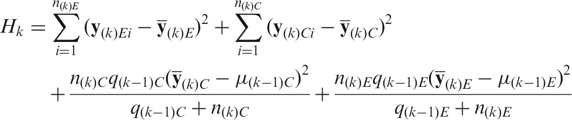
To facilitate interim SSR, the design described in the above section can be adapted. The required sample size (N) is now gathered in K stages. Let $n_{(k) j}$ represent the sample size recruited in group j (where $j = E, C$ and $n_{k} = \sum_{j} n_{(k) j}$ ) in the kth stage, with $k = 1, \dots, K$ . Equal allocation is assumed and interims are not required to be equally spaced.

At each interim, distributions of the precision (ν) and the means (μ_j) are updated with the collected data. The prior value of a parameter at the kth interim will now be referred to with subscript k − 1. Consequently, the subscript for the posterior, updated value can be denoted by k. This value is equal to the prior for the k + 1th interim. Note that k = 0 corresponds to the design phase and subscript K refers to the posterior value of the parameter if all the required sample size is recruited.

The posterior of $μ_{j} | ν$ has parameters $μ_{(k) j} = μ_{(k - 1) j} (q_{(k - 1) j} / q_{(k) j}) + n_{(k) j} {\bar{y}}_{(k) j} / q_{(k) j}$ and $q_{(k) j} = q_{(k - 1) j} + n_{(k) j}$ , where ${\bar{y}}_{(k) j}$ is the mean of the data collected in group j in the kth stage. The gamma posterior of ν has parameters $α_{k} = α_{k - 1} + n_{k} / 2$ and $β_{k} = β_{k - 1} + H_{k} / 2$ where

\begin{matrix} H_{k} = \sum_{i = 1}^{n_{(k) E}} (y_{(k) Ei} - {\bar{y}}_{(k) E})^{2} + \sum_{i = 1}^{n_{(k) C}} (y_{(k) Ci} - {\bar{y}}_{(k) C})^{2} \\ + \frac{n_{(k) C} q_{(k - 1) C} ({\bar{y}}_{(k) C} - μ_{(k - 1) C})^{2}}{q_{(k - 1) C} + n_{(k) C}} + \frac{n_{(k) E} q_{(k - 1) E} ({\bar{y}}_{(k) E} - μ_{(k - 1) E})^{2}}{q_{(k - 1) E} + n_{(k) E}} \end{matrix}

The posterior of $δ | ν$ has mean $δ_{k} = μ_{(k) E} - μ_{(k) C}$ and precision $D_{k} ν$ , with $D_{k} = (q_{(k) E} q_{(k) C}) / (q_{(k) E} + q_{(k) C})$ .

As the trial progresses, the relative influence of the trial data increases, and that of the initial prior belief decreases. This reflects the inherent updating nature of the Bayesian methodology. At interim k, the additional sample size required to obtain the design characteristics (N_k) now depends on the last posterior value of α and D

D_{K} \frac{α_{K}}{β_{k}} (1 - {Beta}_{\frac{N_{k}}{2}, α_{k}, ξ}) \geq (\frac{t_{2 α_{K}, ζ} + t_{2 α_{K}, η}}{δ^{*}})^{2}

(5)

where

D_{K} = (q_{(K) E} q_{(K) C}) / (q_{(K) E} + q_{(K) C})

and

α_{K} = α_{k} + N_{k} / 2

. The total required sample size (as estimated at stage k, including those already measured) is equal to

N_{k} + \sum_{p = 1}^{k} n_{p}

2.2 ξ Calculation

As mentioned earlier, ξ represents the probability of a conclusive decision by the end of the trial. By solving equations (4) and (5) for ξ, we can calculate this probability, given the prior, the data so far, and the remaining sample size.

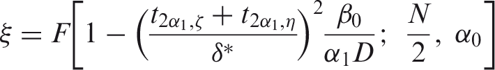
When equation (4) is solved for ξ, we obtain

ξ = F [1 - (\frac{t_{2 α_{1}, ζ} + t_{2 α_{1}, η}}{δ^{*}})^{2} \frac{β_{0}}{α_{1} D}; \frac{N}{2}, α_{0}]

where

F (x; a, b)

is the c.d.f. of a Beta distribution with parameters a and b.

By applying the same steps to equation (5), we can also find an expression for ξ_k in a setting with multiple interims

ξ_{k} = F [1 - (\frac{t_{2 α_{K}, ζ} + t_{2 α_{K}, η}}{δ^{*}})^{2} \frac{β_{k}}{α_{K} D_{K}}; \frac{N_{k}}{2}, α_{k}]

(6)

In the case of limited available sample units, if the required sample size cannot be recruited, ξ_k can be used to evaluate the consequences of continuing the trial with the maximum available subjects. Moreover, the benefit of putting in the extra effort to recruit more subjects can now be quantified. In the following section, the operational characteristics of ξ are evaluated and the impact of a misspecified prior for the variance is assessed and shown to be substantial. The application of PDCCPP’s is demonstrated, as well as how they can be used as a remedy.

The importance of SSR for such a Bayesian approach is stressed. In addition to the reasons sketched for the frequentist case (i.e. the variance being poorly described by the prior distribution due to systematic differences in the two populations), the uncertainty about the variance is now, unlike in the frequentist case, directly incorporated in the sample size calculation. This results in larger sample sizes required for similar decision thresholds (as can be seen when comparing equation 4 with equation 1 for $σ_{0}^{2} = β_{1} / α_{1}$ ). By incorporating interim data in the variance estimation, this uncertainty is reduced resulting in a re-estimated sample size smaller than the initial one, also when the expected value for the precision is the same.

This is shown in Table 1. For the situation where δ^*= 0.6, η = 1 − α = 0.95, ζ = 1 − β = 0.8, ξ = 0.9 and only a prior on the variance is used (thus the priors for the groups’ means are non-informative), the sample sizes calculated are compared with the frequentist one. In the frequentist case, a

σ_{0}^{2} = 1

is assumed while in the Bayesian case a gamma prior distribution around ν is used with E(ν) = 1, α₀ = 5, and β₀ = 5. It is shown how SSR in a Bayesian RCT of this kind can decrease the, initially considerably larger, sample size if the variance is as expected. Here N_I denotes the sample size at which the interim takes place, but it is equivalent to the situation where the prior for ν is based on N_I. As such N_I may be larger than N_Bayes.

Table 1.

Sample size required for frequentist and Bayesian procedures for δ^*= 0.6, η = 1 − α = 0.95, ζ = 1 − β = 0.8, ξ = 0.9.

N_I	N_freq	N_Bayes
0		140
10		108
20		96
30	72	90
40	72	86
50		82
100		80
500		72

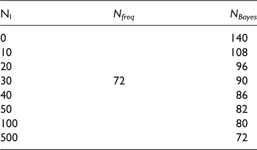
Note: N_I denotes the sample size at which the interim analysis takes place (or the size of the prior if N_I > N_Bayes – see text for details) while the mean of $ν | N_{I} = σ_{0} = 1$ . The initial prior (a gamma distribution with α₀ = 5 and β₀ = 5), corresponding to N_I = 0, is based on a historical dataset of 10 patients. The priors for the groups’ means are taken to be non informative (q₀ _E = q₀ _C = 0).

Here we mention that comparison of Bayesian and frequentist sample sizes is by no means straightforward. Nevertheless the mathematical resemblance of equation (1) with equation (2) allows us to make such a comparison and note that the frequentist paradigm is similar to the Bayesian approach described here, if it were to assume that the mean of the posterior of ν is known and equal to $α_{1} / β_{1}$ .

3 Frequentist properties of Bayesian SSR

3.1 Variance misspecification

From now on, even though modelling takes place in terms of precision (ν), we describe dispersion by the standard deviation σ for purposes of standardization and clarity. As shown in the previous section, Bayesian SSR can aid to mitigate the inflation on the initial sample size calculation imposed by modeling the uncertainty about σ. However, if the true σ, σ_R is different than the one observed in the historical data $(σ_{0} = \sqrt{\frac{β_{0}}{α_{0}}})$ , the Bayesian procedure can have unpredictable operational characteristics.

For our illustrative case, when design parameters are as introduced in the previous section, Figure 1 shows the sample size estimated when the mean of the prior is $E (ν) = 1$ , so $E (σ) \approx 1$ , but σ_R is not as expected, for different sizes of the prior and interim location. Especially when the true variance is larger than expected, the prior distribution can cause considerable discrepancies in the estimated sample size, even when SSR is employed.

Figure 1.

Sample sizes estimated with Bayesian SSR, with their 95% confidence intervals, for different true σ’s (σ_R), for assumed σ = 1 and δ^*= 0.6, η = 1 − α = 0.95, ζ = 1 − β = 0.8, ξ = 0.9, q₀ _E = q₀ _C = 0. The prior distribution is based on either 10 (left) or 20 (right) patients.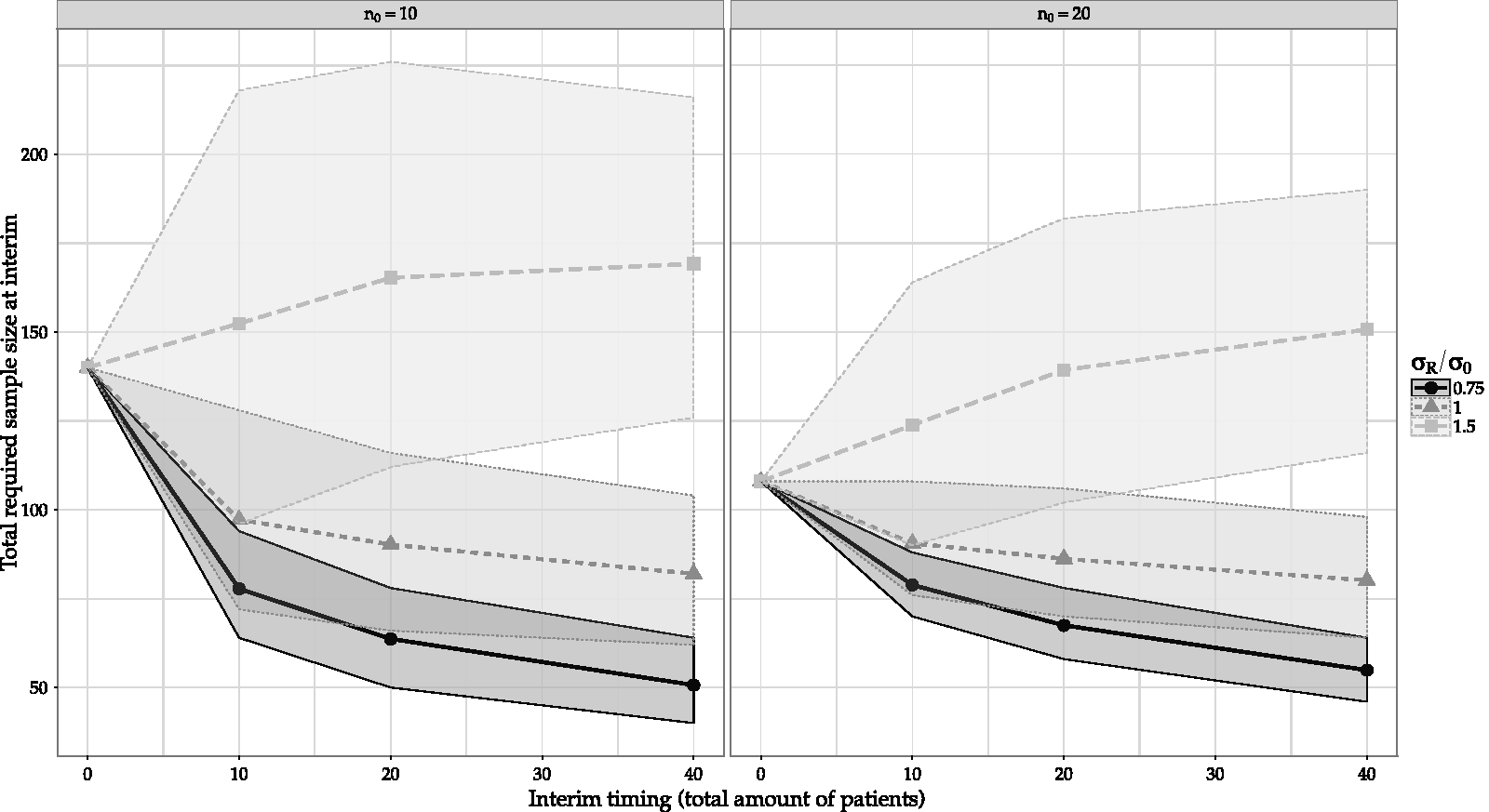

These issues become more apparent when the frequentist properties of ξ are studied. The top two panes of Figure 2 shows the empirical ξ (ξ_emp), that is the empirical probability of equation (2) being satisfied (calculated using equation (6)), as a function of the ratio of the (re-)estimated sample size (i.e. the collected sample size divided by the sample size (re-)estimated at interim that is required to obtain the design characteristics ( $ξ_{emp} = 0.9$ ). Plotted for different interim sizes and σ_R, such a metric explores how reliably equation (6) can estimate the frequentist probability of making a decision with the sample size estimated by the Bayesian approach. It is evident that such calculations are significantly unstable and heavily influenced by both the location and scale of the prior distribution.

Figure 2.

Empirical probabilities of making a decision (ξ_emp) when sample size is (re-)estimated without (top) or with (bottom) calibration using PDSCCPP’s for different ratios of true σ (σ_R) over assumed at design stage (σ₀), for assumed σ = 1 and δ^*= 0.6, η = 1 − α = 0.95, ζ = 1 − β = 0.8, ξ = 0.9, q₀ _E = q₀ _C = 0. The prior distribution is based on either 10 (left) or 20 (right) patients.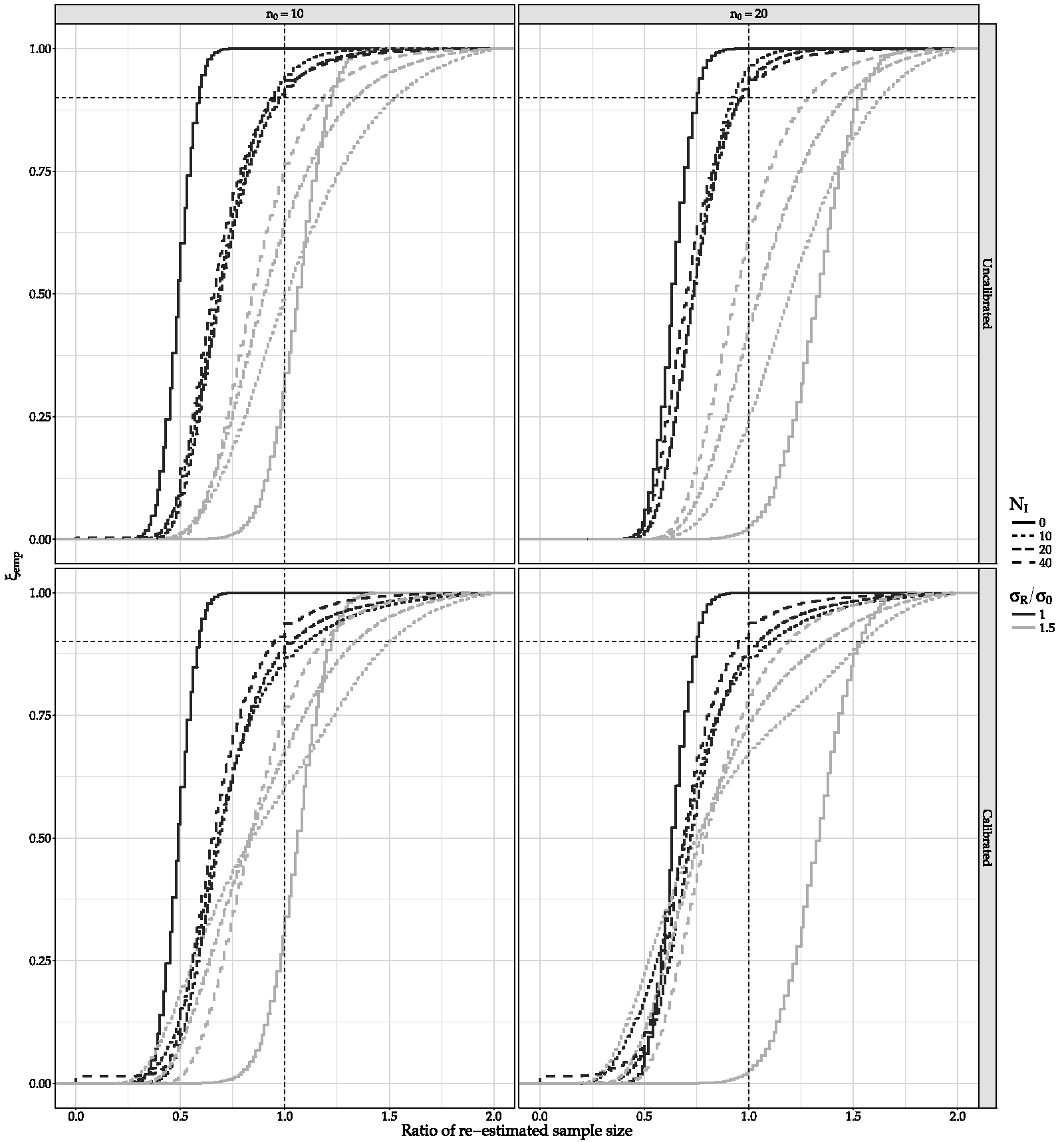

The problem is only partially remedied by re-estimation and/or increasing the interim size and even then, when the true variance is larger than expected by the prior, ξ_emp is deviating considerably from its 90% assumed value for the sample size (re-)estimated. When $σ_{R} = σ_{0}$ we see that equation (2) is true roughly 90% of the times at the sample size re-estimated, in accordance with the design requirements. This holds irrespective of the size of the prior distribution and the interim look location. But when $σ_{R} = 1.5 σ_{0}$ , the sample size required to make a decision with probability as by design ( $ξ = 90 %$ ) can be considerably larger than the one (re-)estimated.

Clearly, deviations from assumptions imposed by the prior distribution can cause calculations which are very relevant for the planning of such a Bayesian RCT, to be untrustworthy. A remedy is suggested by using adaptive power priors which calibrate the prior distribution in light of the new data, thus circumventing the problem.

4 Prior data conflict calibrated power priors

If the data of a current study is denoted by D₁ with respective likelihood function $L (θ | D_{1})$ where θ is a vector of parameters and D₀ denotes the data from a similar historical study, with $L (θ | D_{0})$ the corresponding likelihood, the basic definition of the power prior as described in Ibrahim and Chen²⁵ is

π (θ | D_{0}, γ) \propto L (θ | D_{0})^{γ} π_{0} (θ)

where

π_{0} (θ)

is the initial prior before the historical data are observed, usually assumed flat. Using this formulation, the posterior of θ after observing D₁ is then

π (θ | D_{1}, D_{0}, γ) \propto L (θ | D_{1}) L (θ | D_{0})^{γ} π_{0} (θ)

(7)

The γ parameter, $\in [0, 1]$ , plays the role of a discounting factor, translating to the proportion of the sample size of the historical study at which the prior is finally based. Several extensions have been discussed in the literature and we refer the interested reader to Ibrahim et al.³¹ Here we employ the one suggested by Nikolakopoulos et al.,²⁹ for its simplicity and adaptive nature. An additional attractive feature of PDCCPP’s is that in conjugate models the posterior in equation (7) is still tractable as γ is replaced by $\hat{γ}$ . The approach can be described as follows: if T is a (sufficient) statistic for θ and $[l_{1 - c / 2}^{pr}, l_{c / 2}^{pr}]$ is a 100(1-c)% credible interval from the prior predictive distribution for θ then

{\hat{γ}}_{PDCCPP} (c) = min [{max}_{\hat{γ}} ({\hat{γ} : T^{obs} \in (l_{c / 2}^{pr}, l_{1 - c / 2}^{pr}) | \hat{γ}}, 1)]

(8)

Thus, the prior is calibrated in such a way so that the 100(1 − c)% predictive credible interval for T includes the observed value T^obs. Or, in other words the $π (θ | D_{0}, \hat{γ})$ is such that the two-sided prior predictive p-value for T is at least c. By choosing c, as shown by Nikolakopoulos et al.,²⁹ one can calibrate the procedure in order for desirable frequentist characteristics to be achieved. Since the above formulation is the only one discussed here, we use the terms ${\hat{γ}}_{PDCCPP}$ and $\hat{γ}$ interchangeably.

4.1 Application of PDCCPP in Bayesian SSR

In order to apply the PDCCPP methodology in the Bayesian SSR problem, we use the predictive distribution for M (see equation (3)). It can be shown that, if the initial priors before the historical study are assumed flat and only information for the variance is used at the design stage, such an empirical power prior formulation is equivalent to using a prior $Gamma (\hat{γ} α_{0}, \hat{γ} β_{0})$ for ν and hence $Var (ν | \hat{γ}) = \frac{1}{\hat{γ}} Var (ν | γ = 1)$ and $E (ν | \hat{γ}) = E (ν) = E (ν | γ = 1)$ where the prior $π (ν | γ = 1)$ is equivalent to full borrowing of the prior data and not implementing PDCCPP.

Analytical derivation of ${\hat{γ}}_{PDCCPP}$ is not straightforward due to the complex form of the cumulative distribution and quantile functions of the F distribution. Nevertheless, estimation of the power parameter by simulation is an easy task. After c is chosen, a simple search procedure with reasonable precision can be employed in order to find ${\hat{γ}}_{PDCCPP}$ . If $M^{obs} > l_{1 - c / 2}^{F_{pr}}$ , where $l_{1 - c / 2}^{F_{pr}}$ is the $1 - c / 2$ quantile of the $F_{pr} (N_{1}, 2 α_{0})$ predictive distribution for M when N₁ patients’ responses are observed (such that $\Pr_{F_{pr}} (M < l_{1 - c / 2}^{F_{pr}}) = 1 - c / 2$ ), $\hat{γ}$ will be such that F_pr will be wide enough (by decreasing the second degrees of freedom parameter to $2 \hat{γ} α_{0}$ ) so that $M^{obs} = l_{1 - c / 2}^{F_{pr}}$ . The counterpart adjustment takes place when $M^{obs} < l_{c / 2}^{F_{pr}}$ . Note that the latter (adjusting F_pr so that $M^{obs} = l_{c / 2}^{F_{pr}}$ when $M^{obs} < l_{c / 2}^{F_{pr}}$ ) might not be possible if M^obs is close to 0. In these cases, in our simulations, we set ${\hat{γ}}_{PDCCPP} = {\hat{γ} : \hat{γ} α_{0} = 1}$ . If $l_{c / 2}^{F_{pr}} \leq M \leq l_{1 - c / 2}^{F_{pr}}, \hat{γ} = 1$ .

The choice of c should be such that the frequentist characteristics of interest are controlled. In this case, a predefined probability of making a decision with the estimated sample size is the key characteristic to satisfy. Note that the larger c is, the narrower the credible interval in equation (8) and consequently, the less probable to use the prior in full. In Nikolakopoulos et al.,²⁹ it is discussed how c has to be larger, the smaller N₁ is relative to the historical sample size (2α₀ in this case), for a procedure based on PDCCPP to preserve the same operational characteristics. Thus, all else being equal, for larger historical sample sizes, larger c’s should be employed in order for the same operational characteristics to be met. We make this choice heuristically here, based on this principle, and elaborate further in section 5.

Figure 2 shows how the operational characteristics of Bayesian SSR turn out to be when PDCCPP are employed. The sample sizes (re-)estimated are now less sensitive to the prior distribution. Calculation of ξ is also more robust as the lines move closer together, with a higher ξ reached in most cases when all of the re-estimated sample size is collected. For example, for the case of N₁ = 40, n₀ = 20, and σ_R/σ₀ = 1.5, empirical ξ goes from 59% without calibration to approximately 80% when calibrated through PDCCPP. Here 1 − c/2 was set to 0.2, 0.4, 0.6 and 0.8 for a ratio of the interim location over the prior of 0.5, 1, 2 and 4, respectively, a heuristic choice as discussed above. In general, c must be such that the empirical ξ does not depend heavily on the true value of the variance and is relatively close to the intended value (here 90%). The implemented value of c will depend on the location and precision of the prior, the true value of the variance and the required robustness of ξ. Since these dependencies are not straightforward to quantify, a simulation-based approach must be implemented. Currently, simulation-based choices for parameters are increasingly applied when designing clinical trials. In the following section, by means of an example, we show how such choices can be more refined.

SSR with or without PDCCPP did not affect operational characteristics such as the probability of showing efficacy or futility (see supplementary material). R code used for the procedure and simulations described in this section as well as the analyses presented in section 5 can be found at https://github.com/timobrakenhoff/BayesianSSRwithPDCCPP.

5 Example

The following example is from a multicentre, double-blind, prospective, randomized, placebo-controlled trial that evaluated the efficacy of dexamethasone in very young patients mechanically ventilated for lower respiratory infection caused by respiratory synctial virus (RSV-LRTI).³² Eighty-five children younger than 24 months on mechanical ventilation were randomized to receive either dexamethasone (E) or placebo (C). The primary outcome measure was the duration of mechanical ventilation in days which was assumed normally distributed in the original trial.

Even though no adequate treatment has yet been identified for severe RSV-LRTI, a previous RCT by van Woensel et al.³³ found a potential beneficial effect of corticosteroids. Treatment with prednisolone as compared to placebo reduced the duration of mechanical ventilation in a small subgroup of patients on mechanical ventilation by 1.6 days. This result was based on seven patients in the prednisolone group and seven patients in the placebo group, for which the estimate for the standard deviation was σ₀ = 4.23.

In order to illustrate the design approach suggested by combining SSR and PDCCPP’s, we discuss the situation where the RCT at hand was to be designed in the Bayesian manner described in Whitehead et al.,⁸ when only prior information on the variance were to be used. Thus, by assuming α₀ = 7, β₀ = 125.3, δ^*= 1.5, η = 0.95, ζ = 0.8 and ξ = 0.9, a sample size of 352 is deemed necessary for a Bayesian RCT that will declare efficacy based on posterior probabilities. This sample size is considerably larger than the 198 patients required by the frequentist approach since the uncertainty about the variance is also modelled. However, as discussed, SSR can reduce the sample size required (if the variance is as assumed). But, if the variance is not as expected by the prior, calculations are not to be trusted. Thus PDCCPP is employed as a remedy.

Figures 3 and 4 show the type of exploration that could be of help in deciding the value of c and the interim timing. The ratio of the (re-)estimated sample size to have a ξ = 90% probability of making a decision as dictated by design, is explored. This ratio can alternatively be expressed as the total number of subjects actually required to reach ξ = 90% divided by the total (re-)estimated number of subjects that were expected to be required at interim. In Figure 3 it is plotted as a function of the ratio of σ_R/σ₀, for different widths of the predictive distribution’s credible interval (PI) and sample sizes at which the interim analysis takes place. In Figure 4 it is plotted as a function of the width of the PI, for different σ_R/σ₀ and interim sample sizes.

Figure 3.

Ratio of (re-)estimated sample size required to reach ξ = 0.9 without (upper) and with (lower) use of PDCCPP. Shown as a function of the true variance for different widths of the prior predictive intervals (1 − c/2) and different sample sizes at which the (re-)estimation takes place N_I = {0, 20, 50}.

Figure 4.

Ratio of (re-)estimated sample size required to reach ξ = 0.9 without (upper) and with (lower) use of PDCCPP. Shown as a function of the width of the prior predictive interval (1 − c/2), for different values of the true variance and different sample sizes at which the (re-)estimation takes place N_I = {0, 20, 50}.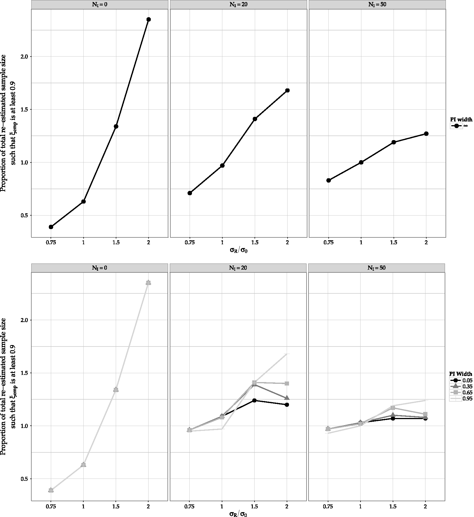

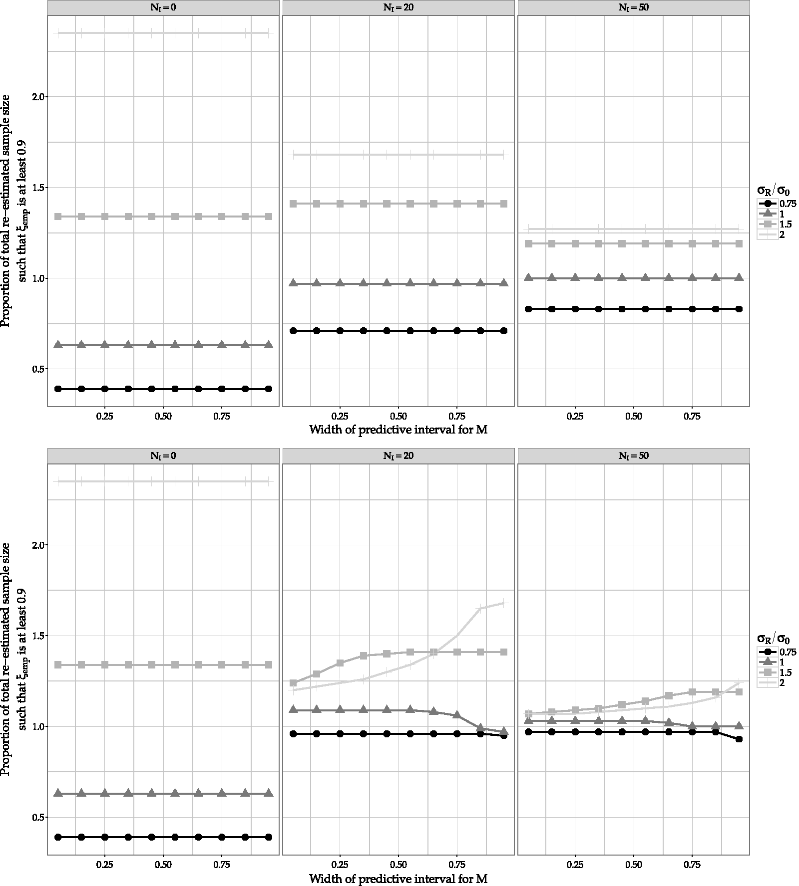
In both figures it is shown how these factors affect the frequentist performance of ξ. The wider the PI is, the less the weight of the prior is adapted. This leads to more biased calculation of ξ (sample size required for 90% probability of making a decision is considerably different). The narrower the PI is, the less the frequentist performance of ξ depends on the true value of the variance (lines in both graphs are closer to each other). Note that at the lower middle plane of Figure 4, when σ_R = 2σ₀, smaller PI widths lead to better ξ estimation than when σ_R = 1.5 σ₀. This happens because the discrepancy between the prior and σ_R (when σ_R = 2σ₀) is such that there is small overlap between the sampling and predictive distributions, leading to higher chances of considerably down-weighting the prior. When the width of the PI becomes large enough, the effect of the large discrepancy takes over, leading to more biased estimation of ξ than when σ_R = 1.5 σ₀.

Such explorations could lead to a choice of PI width and interim timing should result in a required balance between variability in sample size calculation and robustness of the calculation of ξ. This can be done alongside considerations about the maximum sample size available in the case of an RCT in small populations.

6 Discussion

In this paper, the sample size determination procedure described in Whitehead et al.⁸ has been adapted to facilitate interim SSR based on the variance of the observed data. Furthermore, the frequentist properties of such a procedure were shown to be heavily dependent on the prior-data disagreement. A power prior method that calibrates the prior in case of conflict is suggested as a solution. It is also discussed how the interplay between the desired similarity and the ratio of the sample sizes of the prior and new data affect those frequentist properties.

As frequentist properties we considered the probabilities of making a decision within the Bayesian decision scheme suggested in Whitehead et al.⁸ Robustness of calculations can be of importance in research conducted in small populations where recruitment difficulties can result to very long clinical trials. Feasibility of such an ongoing trial is of interest.

We did not dwell into probabilities of correct or wrong decisions (the analogues of type I and II errors). However, as shown in the supplementary material, such probabilities were only marginally affected by the SSR suggested here. This does not come as a surprise since our method is monitoring only the variance and not the treatment effect. Methods that facilitate SSR by monitoring the variance are generally more well accepted by regulators.⁶ It should be noted that the current method requires unblinding, at least of the statistician.

We also encourage further research on the performance of this method when multiple interim looks are taken sequentially and the allocation of sample size is not 1:1. While the sample size re-estimation method proposed here is explored for multiple interims, we would advise the detailed attention of a statistician at the end of each interim (which can be considered best practice). If this is not possible, we propose to perform no more than 1 interim when interested in performing Bayesian sample size re-estimation with PDCCPP. Limited increase in efficiency, risk of unintended bias, and other logistical concerns may also be reasons to restrict the number of interims. In addition, the allocation of sample size in this paper is assumed to be 1:1. However, as the original Bayesian sample size estimation approach proposed by Whitehead et al.⁸ does not require equal allocation, this assumption can likely be relaxed in the re-estimation approach proposed here.

The Bayesian method explored here results in considerably larger sample sizes than the frequentist ones for seemingly similar decision criteria. We show how SSR can partly remedy this. Assuming that the uncertainty in any variance estimate (prior distribution or fixed assumption) is acknowledged, and SSR is part of the design of a new trial, the Bayesian and frequentist approaches suggest two different strategies: Let us consider the case where a two-stage SSR is planned (thus one interim analysis for SSR) for a trial with very limited prior information, for example one small pilot study. A frequentist would start small, bearing considerable uncertainty concerning the sample size estimate of the second stage. The amount of this uncertainty depends on the sample size of the pilot study. Furthermore this uncertainty is not incorporated in the assumed value for the variance thus the sample sizes calculated might be deemed as unrealistic in small populations RCTs.

A Bayesian would start large, thus being prepared in terms of commitment of resources, and then reduce the sample size if the true variance was indeed equal to the point estimate of the pilot study – the same estimate the frequentist would use. The PDCCPP approach is fairly robust against variance misspecification; a robustness all more important in RCTs in populations where repetition of a trial that was subject to misspecification is rather unlikely. The Bayesian would also have a different decision scheme as posterior inference as described in Whitehead et al.⁸ could also conclude futility whereas “acceptance of H₀” is not very popular amongst frequentists.

In both the frequentist and Bayesian approaches, one can think of intuitively awkward issues. In the frequentist approach, the sample size is calculated under the assumption of a value for the unknown variance. In the Bayesian one, empirical ξ is far from the one calculated. This is not surprising as a single value for ν is not the data generating mechanism assumed in the Bayesian model. This discrepancy reduces the larger the new data is relatively to the old. It is hard to imagine a data-generating mechanism that depends on how much knowledge one has for its parameters.

We try to bridge these gaps by an application of the PDCCPP. Essentially an Empirical Bayes methodology, it facilitates both the Bayesian belief and the frequentist operational characteristics in the design and analysis of a clinical trial. We argue that these are both features that could be of interest in conducting research in small or sensitive populations.

Supplemental Material

Supplemental material for Bayesian sample size re-estimation using power priors

Supplemental material for Bayesian sample size re-estimation using power priors by TB Brakenhoff, KCB Roes and S Nikolakopoulos in Statistical Methods in Medical Research

Footnotes

Declaration of conflicting interests

The author(s) declared no potential conflicts of interest with respect to the research, authorship, and/or publication of this article.

Funding

The author(s) disclosed receipt of the following financial support for the research, authorship, and/or publication of this article: This study was supported by the European Union’s seventh framework programme (FP7-HEALTH-2013-INNOVATION-1, Grant-Agreement No. 603160, ASTERIX).

Supplemental material

Supplemental material for this article is available online.

References

Friede

Miller

. Blinded continuous monitoring of nuisance parameters in clinical trials. J Royal Stat Soc: Series C (Appl Stat) 2012; 61: 601–618.

Gould

. Sample size re-estimation: recent developments and practical considerations. Stat Med 2001; 20: 2625–2643.

Jennison

Turnbull

. Group sequential methods with applications to clinical trials, Boca Raton, USA: Chapman & Hall/CRC, 2000.

Denne

. Sample size recalculation using conditional power. Stat Med 2001; 20: 2645–2660.

Mehta

Tsiatis

. Flexible sample size considerations using information-based interim monitoring. Drug Inform J 2001; 35: 1095–1112.

U.S. Department of Health and Human Services, Food and Drug Administration, et al. Guidance for industry: adaptive design clinical trials for drugs and biologics (Draft guidance) 2010 2010. https://www.fda.gov/downloads/drugs/guidances/ucm201790.pdf .

Gould

. Planning and revising the sample size for a trial. Stat Med 1995; 14: 1039–1051.

Whitehead

Valdés-Márquez

Johnson

, et al. Bayesian sample size for exploratory clinical trials incorporating historical data. Stat Med 2008; 27: 2307–2327.

Brown

Herson

Atkinson

, et al. Projection from previous studies: a Bayesian and frequentist compromise. Control Clin Trials 1987; 8: 29–44.

10.

Lecoutre

. Two useful distributions for Bayesian predictive procedures under normal models. J Stat Plan Inference 1999; 79: 93–105.

11.

Lee

Zelen

. Clinical trials and sample size considerations: another perspective. Stat Sci 2000; 15: 95–110.

12.

Spiegelhalter

Freedman

Parmar

. Applying Bayesian ideas in drug development and clinical trials. Stat Med 1993; 12: 1501–1511.

13.

Berry

Carlin

Lee

, et al. Bayesian adaptive methods for clinical trials, Boca Raton, USA: CRC Press, 2010.

14.

Claxton

Lacey

Walker

. Selecting treatments: a decision theoretic approach. J Royal Stat Soc: Ser A (Stat Soc) 2000; 163: 211–225.

15.

Sahu

Smith

. A Bayesian method of sample size determination with practical applications. J Royal Stat Soc: Ser A (Stat Soc) 2006; 169: 235–253.

16.

Stallard

. Sample size determination for phase II clinical trials based on Bayesian decision theory. Biometrics 1998; 54: 279–294.

17.

Joseph

Wolfson

Du Berger

. Some comments on Bayesian sample size determination. Statistician 1995; 44: 167–171.

18.

Pezeshk

. Bayesian techniques for sample size determination in clinical trials: a short review. Stat Meth Med Res 2003; 12: 489–504.

19.

Pham-Gia

Turkkan

. Sample size determination in Bayesian analysis. Statistician 1992; 41: 389–397.

20.

Gould

. Interim analyses for monitoring clinical trials that do not materially affect the type I error rate. Stat Med 1992; 11: 55–66.

21.

Wang

. Sample size reestimation by Bayesian prediction. Biometric J 2007; 49: 365–377.

22.

Hartley

. Adaptive blinded sample size adjustment for comparing two normal meansa mostly Bayesian approach. Pharmaceut Stat 2012; 11: 230–240.

23.

Hartley

. A Bayesian adaptive blinded sample size adjustment method for risk differences. Pharmaceut Stat 2015; 14: 488–514.

24.

Zhong

Koopmeiners

Carlin

. A two-stage Bayesian design with sample size reestimation and subgroup analysis for phase II binary response trials. Contemporary Clin Trials 2013; 36: 587–596.

25.

Ibrahim

Chen

. Power prior distributions for regression models. Stat Sci 2000; 15: 46–60.

26.

De Santis

. Using historical data for Bayesian sample size determination. J Royal Stat Soc, Ser A 2007; 170: 95–113.

27.

Hobbs

Carlin

Mandrekar

, et al. Hierarchical commensurate and power prior models for adaptive incorporation of historical information in clinical trials. Biometrics 2011; 67: 1047–1056.

28.

Gravestock

Held

. Adaptive power priors with empirical Bayes for clinical trials. Pharmaceut Stat 2017; 16: 349–360.

29.

Nikolakopoulos S, van der Tweel I and Roes K. Dynamic borrowing through empirical power priors that control type I error. Biometrics Epub ahead of print 11 December 2017. DOI: 10.1111/biom.12835

30.

Gsponer

Gerber

Bornkamp

, et al. A practical guide to Bayesian group sequential designs. Pharmaceut Stat 2014; 13: 71–80.

31.

Ibrahim

Chen

Gwon

, et al. The power prior: theory and applications. Stat Med 2015; 34: 3724–3749.

32.

van Woensel

Van Aalderen

De Weerd

, et al. Dexamethasone for treatment of patients mechanically ventilated for lower respiratory tract infection caused by respiratory syncytial virus. Thorax 2003; 58: 383–387.

33.

van Woensel

Wolfs

Van Aalderen

, et al. Randomised double blind placebo controlled trial of prednisolone in children admitted to hospital with respiratory syncytial virus bronchiolitis. Thorax 1997; 52: 634–637.

Supplementary Material

Please find the following supplemental material available below.

For Open Access articles published under a Creative Commons License, all supplemental material carries the same license as the article it is associated with.

For non-Open Access articles published, all supplemental material carries a non-exclusive license, and permission requests for re-use of supplemental material or any part of supplemental material shall be sent directly to the copyright owner as specified in the copyright notice associated with the article.

0.00 MB

0.10 MB