Speaking Stata: The largest five—A tale of tail values

Abstract

How do you work with the largest five, or smallest five, or any other fixed number of values in a tail of a distribution? In this column, I give examples of problems and code for basic calculations as a prelude to graphics, tables, and more detailed analysis. The main illustration is analysis of concentration among firms or companies, with wider discussion mentioning hydrology, climatology, cryptography, and ecology. The examples allow a tutorial covering sorting and ranking and using if and in to select observations, by: as a framework for groupwise calculations, indicator variables as a mode of selection, and egen as a Swiss Army knife with many handy functions.

1 Introduction

Faced with a distribution, researchers may want to look systematically at (say) the 5 largest or the 5 smallest values. Here 5 is evidently just an example: the same principles apply if the number chosen is 3, 10, 30, or whatever else. Further, 1 is a notable special case.

In economics or finance, we may want to look at the 5 firms with the largest number of employees or sales volume or market value or the 5 best- or 5 worst-performing stocks. In hydrology and climatology, we might want to look at the 5 largest floods (river discharges) or the 5 driest years in terms of rainfalls. Extremes can be interesting and important, to say the least. Think of the Amazon, the world’s largest river on most criteria, or Amazon, a rather large firm.

Stata practice here starts with some very simple devices but necessarily gets more complicated as we face up to common difficulties, including wanting to do this systematically for subsets of the data; coping with missing values; desiring to go beyond simple summaries in further work; and wanting to work efficiently with large datasets.

The idea of “the largest 5” or any variation on that theme is easy to explain to lay people or beginning students. The idea may still be helpful at other levels. If 5 seems arbitrary, there are easy answers: try some other choice instead or as well, or do something else entirely if your problem needs a different solution.

In what follows, it is assumed that ties are not a problem. If the 5 largest values are all 42, that is what it is. For ideas on how to handle distinct values, often called unique values, you could start with Cox and Longton (2008). In practice, when people want to do this, the 5 largest or smallest values commonly are distinct and come from a straggly tail of a skewed distribution.

We will stop a long way short of the statistics of extremes. On that, Gumbel (1958) is the classic account. More recent books include Embrechts, Klüppelberg, and Mikosch (1997), Coles (2001), Beirlant et al. (2004), Reiss and Thomas (2007), and Resnick (2007). Davison and Huser (2015) gave a recent review.

2 Easy commands

Starting with easy commands, let us see how far we can get with summarize, collapse, sort, list, and keep (see [R] summarize, [D] collapse, [D] sort, [D] list, and [D] drop) in particular.

summarize always reports the minimum and maximum. With its detail option, it lists the 4 highest and 4 lowest values, without saving any of those results except the minimum and maximum. summarize can be more useful once observations have been identified as satisfying a particular criterion, as we will see shortly.

collapse lets you collapse to a reduced dataset that could include minimum and maximum values, and whatever else you want, but collapse lacks handles for other values in each tail of a distribution. It can still be helpful after other calculations.

sort on a variable sorts the dataset from lowest to highest values on that variable. For example, with auto.dta, we could go

auto.dta is a small and generally well-behaved dataset. There are no missing values on price, so everything is as simple as it could be. We can now look at the tails of the distribution of price using list. Here are some basic possibilities, starting with a device you should know already and ending with one you may not have seen before.

The in qualifier specifies observation numbers and allows one range of observation numbers. The observation numbers depend on the current sort order, which for this problem is precisely the point. So after sort price, the qualifier in 1/5 identifies the observations with the 5 lowest values of price, and the qualifier in -5/L identifies those with the 5 highest values.

Note especially the use of negative integers to specify observations counting from the bottom of the dataset upward. Stata allows -1 and indeed the letter l to indicate the last observation, but I recommend L (also meaning last). L means one fewer keystroke than -1. Lower case l is all too easily misread as the numeral 1. Using negative numbers surely beats calculations on the fly, such as this: I have 74 observations, so I want to see the last 5, which means in 70/74.

Note that the answer is not in 69/74. A little thought or experiment underlines that such code identifies six observations. My experience is that one never stops making such off-by-one or fencepost errors and thus needing to fix them. If the term is new to you, a quick Google on “fencepost errors” leads to informative sources.

The last code example just given using inrange() is more complicated than you may need, but the idea is sometimes useful. Here _n is the observation number (running from 1 to 74 in auto.dta), and _N is the total number of observations (so 74 in auto.dta). We need _N - 4 at the bottom of the dataset to specify where observations in the top 5 start. In short, if used like this is a way to work around restrictions on the in syntax. We can specify multiple observation number ranges using the | operator, meaning logical or: this | that is true if either this or that is true. See help operators for more detail on logical and other operators.

Sorting has many benefits. We could now use list to look at other variables too on the observations with extreme values, including name, place, or time identifiers and other categorical or measured variables. We could now use summarize with an in qualifier. A detail often overlooked is that summarize calculates the sum as well as other results: although not displayed in results, the sum is available immediately afterward as the saved result r(sum).

You could also use keep to produce a reduced dataset consisting only of observations in either or both tails. This idea too is more useful in more challenging contexts.

3 Comparing subsets

People wanting this usually seek much more. The context is often wanting to look systematically at how “the largest 5” vary in some way, say, how some results vary from year to year. In economics or finance, we might have companies in different economic sectors for a period of years and want to consider variations in some measures between sectors and between years. In environmental science, we might have monitoring stations in different regions over a period of years. And so on.

One more step in technique yields many useful results. The step is to use generate and egen (see [D] generate and [D] egen) as workhorses within a framework provided by the by (see [D] by) prefix. The perspective is now that new variables are needed, so that we can graph, table, and further analyze our results most easily.

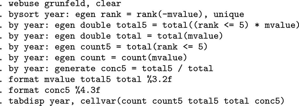
Let’s dive into a more challenging example and then explain the new tricks being used. Suppose we want to look at concentration of economic activity as it varies over time. The Grunfeld data are a good sandbox. Let’s use market value mvalue as a size variable and look at the total mvalue for the largest 5 companies, and that as a fraction of the total mvalue for all companies, as they vary from year to year. The latter is often called a “concentration ratio”. The Grunfeld data include 10 companies, which is not a problem: nowhere will we wire in 10 as part of the code.

The results for our dataset will be shown toward the end of this section.

First off, let me flag that this code capitalizes on there being no missing values in the variables concerned. We will hold until a later section a discussion of how to deal with any missing values.

Next, note that 5 is wired into the code at just one place, although if you used a different integer, it would also be prudent to change some new variable names accordingly. This is not an attempt at very general code. It includes specific details arising from a particular dataset, but we are slowly working our way toward respectable code for a do-file.

To understand the code as a whole, let us work backward from what we want, which is the total market value of the largest 5 companies; the total market value; the ratio of those two totals, which we know will lie between 0 and 1. Preferring that concentration ratio to be a percentage between 0 and 100 is an alternative.

The easiest of these to get at is the total market value for each year, which goes in the new variable total.

For that and the partial total for the largest 5, the code uses double variables. Totals can become very big, so we decide to worry a little about holding total values to maximum precision.

After we sort first by year and then by mvalue, the largest 5 values are in the last 5 observations. The detail used here is to create an indicator or dummy variable that is 1 if the observation is one of the largest 5 and 0 otherwise. It is hard to overstate how useful such variables can be (Cox 2016; Cox and Schechter 2019).

The precise criterion compares the observation number _n with the total number of observations _N. It is crucial that—under the aegis of the by: prefix—these are calculated within each group of observations specified, in this case a distinct year (Cox 2002). Spelling it out, we want the observations with numbers equal to _N, _N − 1, _N − 2, _N − 3, and _N − 4.

Consider this statement:

• by year: egen double total5 = total(highest * mvalue)

Multiplying by highest means that we are adding terms that are 1×mvalue when in the largest 5 together with terms that are 0 × mvalue when not in the largest 5. That boils down easily to the total of mvalue for the observations that make up the largest 5 in any subset. Getting a clean expression for selection of observations and multiplication is a nice possibility when an indicator variable is to hand.

The code could have been

• by year: egen double total5 = total(mvalue) if highest == 1

or even

• by year: egen double total5 = total(mvalue) if highest

In either case, the result for observations with highest == 0 would be missing. The indicator variable approach appeals, I suggest, as yielding less clumsy code. It reduces the need to keep track of which observations have nonmissing values of total5 and which have missing values.

The variable count5, which is in egen terms total(highest), will similarly be the sum of 1 for each value in the largest 5 and 0 otherwise, which is precisely a count of values in the largest 5, as desired. I have two reasons for calculating this variable.

First, to check on the counting. The result in our dataset should always be 5. But always be on the lookout for off-by-one errors, in which our code could yield 4 or 6. Indeed, worse errors might occur. While working toward this column, I made a careless slip of this kind but caught it quickly because I was counting too.

Second, to look ahead toward the possibility of unbalanced panels with unequal numbers of observations for each year (or time generally). Suppose that there were only 1, 2, 3, or 4 nonmissing values of mvalue in each year. Then total5 would still contain their total; it would also equal total; and the concentration ratio total5 / total would be identically 1. Keeping a count in the variable count5 of the number of values in the “largest 5” lets us watch out for such instances.

A further possibility is that there are only 5 nonmissing values in each year, which would also imply a ratio of 1. For that and other reasons, we also have a variable count, which is the number of nonmissing values available in each subset. See the help for egen on its function count() if you want more detail.

Note on Stata terminology. egen is a framework for running its own routines, called “functions”. Several are bundled with official Stata, and many more have been written by users. Such functions are not the same as functions in Stata proper or in Mata (Cox 2011b). Sorry if this is confusing or irritating, but three different names for varieties of the same idea might well have been just as confusing or irritating.

The results for our new variable are identical for each observation in the same subset, so in this example for each year. That smacks of redundancy but is otherwise convenient. Readers familiar with frames (introduced in Stata 16) will be aware of another approach, and indeed the problem could also be recast using Mata. Identical results for each observation in each year, however, do mean that we want to see each distinct line of results only once. It is one of many small virtues of tabdisp (see [P] tabdisp) used for tabular display that this behavior can be automatic.

Repeating the tabdisp command from earlier in this section, we can now think more about how to show the results.

Before the tabdisp command, we assigned display formats to the variables here with noninteger values. Specifying two decimal places for the totals just echoed the resolution of the original data. For any purpose other than checking results, more rounding would be fine. Other way round, three decimal places for the ratio is, I guess, about what people often want to show.

I wanted to show the counts explicitly because some people with messier datasets really need to display them. For this kind of dataset, we should check that counts are as they should be but then suppress the display in a presentation or publication. It would also be a good idea to have checks in the code using assert (see [D] assert) such as

whenever constancy is expected: it is expected here because we think we have balanced panels and no missing values. If either of those commands failed, you would need to find out why. If the explanation made sense, you would then remove the assert commands from the code but ensure that the counts are available to readers of your research. Either way, it pays to be assert ive (Gould 2003).

tabdisp remains a neglected command (Cox 2003, 2012). It can be just what you need for quick and not so dirty display of variables, including results variables. It is billed as a programmer’s command, but it is easy to use interactively and in do-files.

A serious project would not stop here. You should first fire up a line graph and then think what next to do. Because each result is repeated for observations in the same year, it would be good practice to go

4 Which measures?

This section is a digression on the statistical content and context of the example.

People interested in measuring concentration should be concerned with the strengths and limitations of fraction of total composed by the 5 largest values as one of several possible measures. It is enough for the present purpose that some researchers find it simple and useful, but is it too simple, and is it as useful as other measures? A great deal has been written in this territory, and there is much scope for yet more.

Let us sketch one larger context and give a few simple examples of other possibilities. We have in market value a variable quantifying size or frequency or abundance that must be zero or positive. The distribution of such a variable, say y, can be reexpressed as proportions y/Σ y =: p. Such a framework fits many applications, such as letter frequencies in elementary cryptography (Holden 2017; Dooley 2018; Dunin and Schmeh 2020) or abundance of species or taxa generally in ecology (several references in Cox [2005]). In this framework, our measure is just ${\displaystyle {\sum }_{j=1}^5{p}_j}$ , where ranks j follow a convention that 1 means largest and there is no correction for ties.

Again, the choice 5 is arbitrary here and a matter of judgment. We can see this measure as one of a family, given choice of J in ${\displaystyle {\sum }_{j=1}^J{p}_j}$ . In ecology, J = 1—so simply p ₁—has often been used, typically named the Berger–Parker index (Berger and Parker 1970). ¹

Two of several other approaches may be singled out. First comes Σp ² =: R or its complement 1 − R, which is usually named for someone who did not first discover or invent it. Repeat rate, named by Alan M. Turing (Good 1953, 1982), and match probability (MacKay 2003, 267) are good evocative names for R.

Then there is Σ p ln(1/p) =: H, usually named entropy, “a quantity which occurs in many contexts, is invoked in many more, and is given justifications ranging from the axiomatic to the metaphysical” (Whittle 1992, 272).

R and H are not directly comparable, but 1/R and exp(H) have an attractive interpretation as an equivalent number of equally common categories. To see that, note that with k identical proportions, so that each proportion is 1/k, R reduces to 1/k and H reduces to ln k.

There are large and sometimes repetitive literatures in several disciplines on how best to measure and analyze concentration (or diversity, or inequality, to mention only two related terms) for a ranked distribution p_j . There are many examples of how quite simple ideas can be helpful. There are also futile debates about which measure is best (in the absence of criteria for “best”) and naive exercises trusting that all the information in a distribution can be captured by a single scalar. Comments within Cox (2005), although in several senses utterly standard, seem to retain their force. New ideas and frameworks continue to emerge (for example, Leinster [2021]).

None of the above is to deny that direct analysis of a size variable y, through, say, momentor quantile-based summaries, may not be a better idea. As Jeffreys (1961, x)² remarked, “It is sometimes considered a paradox that the answer depends not only on the observations but on the question; it should be a platitude.”

5 Missing values

We postponed discussion of missing values.

Missing values have to be sorted to somewhere in the data. The only systematic choices could be that numeric missing values are regarded as 1) lower than the largest negative value possible or 2) higher than the largest positive value possible. Stata developers made the second choice. It follows that, after sorting, any numeric missing values will compose some of if not all the “largest five”—in the sense that they will be list ed last, or shown last in the Data Editor.

A solution to this problem is just to segregate missing values so that they do not enter the calculation. That is easier than might be feared once you have created an indicator variable for being missing, which then allows a different sort order.

We do not need this refinement for the Grunfeld data, but it does no harm. Here— once we have been more careful about creating an indicator variable highest—most of the code is unchanged.

Note the use of the logical operator and (&). To be regarded as one of the highest, a value must not be missing and in the top 5. this & that is true only if both this and that are true.

6 Ranking instead

Another idea—which may have already occurred to you—is that for our main example of measuring concentration using the largest 5, what we seek are just values with ranks 1 to 5, so long as we can rank in a way that matches the calculation. We can do that directly in Stata.

Here is revised code.

We need to negate the argument to rank()—note the negative sign before mvalue— to ensure that the values are ranked from 1 for largest onward. We also need the unique option to disable the default treatment of ties, which is to assign to tied values the average of ranks that would otherwise have been assigned. These are details to take care of. See the help for the rank() function of egen for details of various flavors of rank.

A positive feature of the rank() function in egen is that missing values are ignored automatically. That is welcome.

You may like this approach more than any so far.

7 Other measures

Naturally, we may want other measures too, whether standard or not. Mean, median, and geometric mean are three attractive summaries for many size measures. The geometric mean applies only to values that are all positive, which is obvious enough here but which may bite for your own application.

Let’s build on the last section and show code for those three. The output is suppressed here but easily reproducible. Again, a line graph is ready to hand. Recall the advice from Section 3 about tagging just one observation for each year.

egen already has functions for mean and median, as you would hope and expect. The trick needed is to limit calculations to observations with ranks 1 to 5. We could use an if qualifier here, which would have few real disadvantages, but choose instead to show off a favorite device, using cond() within a function call to ignore whatever you want to ignore (Cox 2011a). See Kantor and Cox (2005) if you remain puzzled by cond().

Two wider principles about egen calls deserve a flag. Many of its functions feed on expressions, which can be more complicated than a bare variable name. We can use any Stata functions here (although, perhaps surprisingly, not other egen functions). Further, egen functions tend to ignore missing values to the extent appropriate. Both principles are being used in the code above for mean and median. First, we instruct egen to treat data assigned ranks 6 upward as if they were missing. Then, we take a mean or median over values, which calculation will ignore missings.

Official Stata lacks an egen function for geometric means, although one has long been available in the egenmore package on the SSC Archive. A good excuse for any lack is how easy it is to get geometric means in two steps: first, take the mean of logged values, and then, exponentiate that mean. A similar trick would yield harmonic means in two steps.

Wainer (2005, 107) makes a neat point arising out of an analysis of Olympic performances. “The bronze medal time is the median of the top five finishers. The winning time can sometimes not be representative, whereas taking a median of the top five yields a more statistically stable measure.” The point has further applications not only within the wide, wide world of sports but also beyond. See also Wainer, Njue, and Palmer (2000).

8 The smallest five

What about the smallest five? Adapting what has been said already should be simple or can be regarded as an exercise.

The convention in egen, rank() that lowest values rank 1 up is convenient in this case. Note that missing values can still bite, just not as often.

9 Efficiency matters?

With really large datasets, we might need to think more about getting results speedily. Here the main caution is that egen code includes extra bells and whistles that you can avoid if you know what you are doing. So, for example, a total can be obtained using the Stata function sum(), which yields cumulative or running sums. Here we revisit the last such line:

• by year: egen double total5 = total((rank <= 5) * mvalue)

A non-egen solution could be

That’s two lines of code. How could it be faster? If you look inside the previous code with

you will see that the two-step is at the heart of the total() function any way, but if we avoid egen, we avoid many lines that parse user input and cope with yet other details that can be omitted in a direct solution.

10 Conclusion

This column will naturally be most interesting and useful if the examples are close to what you want to do. Beyond that, I have a larger tale to tell.

A serious subject need not entail a solemn or stuffy style. But banter about coding tricks should not distract from a positive theme. Again and again, problems that are simple to understand can be coded up with fairly simple Stata code using a small set of devices and methods, such as

• sorting and ranking

• if and in to select observations

• by: as a framework for groupwise calculations

• indicator variables as a mode of selection

• egen as a Swiss Army knife with many handy functions

Pólya (1957, 208) quipped, on behalf of the “traditional mathematics professor”, “What is the difference between method and device? A method is a device you use twice.” In Stata, as elsewhere, expertise grows as you learn whichever tricks are devices, or even better methods, that you can use again and again in different problems.