Binary contrasts for unordered polytomous regressors

Abstract

In observational studies, regression coefficients for categorical regressors are overwhelmingly presented in terms of contrasts with a reference category. For unordered regressors with many categories, however, this approach often focuses on contrasting different pairs of categories to one another with little substantive rationale for foregrounding some comparisons with others. Mean contrasts, which compare categories with the overall mean, provide an alternative to the reference category, but the magnitude of mean contrasts is conflated with the relative sizes of the categories. Instead, binary contrasts compare a category with all the other categories, allowing the familiar interpretation for dichotomous regressors. Our command binarycontrast computes binary contrasts.

1 Introduction

With unordered polytomous explanatory variables, there is often no reason to consider any one category as being more substantively fundamental for interpreting results than the others. Consider when a categorical explanatory variable is the region of the country where a person lives. There may be no reason to think that comparisons with any particular region are more interesting or important than the comparisons with any other region. Nevertheless, the most common strategy for presenting coefficients for such variables involves assigning one category as the reference category so that coefficients for other categories are identified as the contrasts between each of them and the reference. For regions, one region will often be specified as the reference category for some substantively irrelevant reason, like being first in alphabetical order.

While contrasts between any pair of categories other than the reference can typically be obtained by simple arithmetic, this still takes for granted that the most useful quantities for interpretation are contrasts between pairs of categories. With regions, for example, it may well be that pairs of regions are not the most useful comparisons to foreground at all; instead, it may be more effective to compare each region with the others as a whole.

To this end, an alternative approach is to present coefficients as the contrast of each category with the overall mean, which is sometimes called “weighted effect coding” (te Grotenhuis et al. 2017), “deviation coding”, or (our preference) “mean contrasts” (Johfre and Freese 2021). Mean contrasts do not involve a reference category; instead, each category has its own coefficient. For a variable with k categories,

${\displaystyle \sum _{m=1}^k{p}_m}{\beta }_m=0$

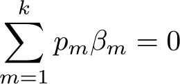
where p_m is the proportion of observations belonging to category m and β_m is that category’s coefficient. (In experimental research, one may simply be interested in results balanced across treatments and thus not weighting by the proportion, but our discussion here is directed to population-based observational studies for which estimates of population proportions are both desirable and able to be estimated from one’s data.)

While interpreting results with the reference category approach involves treating one category as different from the others, with mean contrasts the coefficients all have a uniform interpretation as the difference between that category and the overall conditional mean. With region of residence, for example, mean contrasts would estimate the differences between each region and the country’s overall mean. But this interpretation may also seem a bit peculiar, given that the observations in the category in question also contribute to the overall mean. So with mean contrasts, a category is being contrasted partly with itself. One consequence is that, for mean contrasts, more frequent categories will tend to have coefficients closer to zero simply by virtue of being larger and hence more influential on the resulting mean. More populous regions tend to have smaller mean contrasts because they are more populous. A further implication is that differences in the magnitudes of mean contrasts cannot be interpreted as differences in effect sizes.

If membership in category m was a binary variable, then the interpretation of β_m would be straightforward, along the lines of “living in [region m] is associated with a β_m difference in the outcome compared with those who do not live in [region m].” The value of β_m here would also not depend on the relative frequency of m. Of course, if we were specifically interested only in m versus not-m—that is, interested only in the contrast between one category and everyone else—we could just fit our model with a binary measure instead of a polytomous one. Instead, we want to fit the model with all the categories of our polytomous measure, yet we still want coefficients for each of the k categories to represent the “binary contrast”, that is, the contrast between those observations belonging to that category and those that do not.

In Stata, mean contrasts can be readily computed postestimation in Stata using the contrast command, but binary contrasts cannot. Our command binarycontrast rectifies this by leveraging the option of the contrast command to specify custom contrasts. We will first present an example that illustrates binary contrasts. Then we explain how binary contrasts are computed and how binarycontrast is implemented in Stata.

2 Example

The General Social Survey (GSS) is a biennial probability-based survey of adults in the United States. In the GSS, subjective social standing is assessed on a 10-point scale. We use this as our outcome, and we use race or ethnicity as our explanatory variable. We code race or ethnicity as four categories, in which respondents who identify as Latino are coded as Latino and other respondents are coded by self-identified race as White, Black, or Other. Following Johfre and Freese (2021), we use Latino as the reference category so that the estimated coefficients are positively signed. We fit the following regression model in Stata:

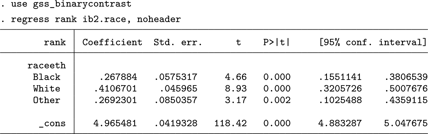
When we look at the coefficients for race or ethnicity, we can see that being White is associated with the highest average subjective rank and being Latino is associated with the lowest. For Black respondents, we note that the coefficient is closer to Whites than it is for Latinos. Does this mean that Black respondents have higher subjective social status than respondents who are not Black? There are more Whites than Latinos in the United States, so the larger difference between Blacks and Latinos might be more than offset by the larger number of Whites and their disproportionate influence on the mean of non-Black respondents. One could thus reasonably look at the coefficients and not know if being Black is positively or negatively associated with the outcome.

We could instead calculate mean contrasts postestimation using contrast:

The result indicates that being Black is indeed negatively associated with lower subjective standing relative to the mean. Meanwhile, the result for Latinos is much farther from zero than any of the other race or ethnic groups and nearly four times as large in magnitude as the difference for Whites. Does this mean that the difference between Latinos and non-Latinos is in fact larger than the difference between Whites and non-Whites? From the mean contrasts, we cannot tell. There are more Whites than Latinos in the GSS, so the reason that the difference is so much smaller for Whites than Latinos could be that there are many more Whites in the sample.

Furthermore, to interpret the mean contrast of 0.083 for Whites, we might say something like, “Being White is associated with a 0.08-point increase in subjective social rank relative to the mean.” Notice, however, that this result is effectively comparing Whites with another “group” that is mostly composed of Whites (that is, the whole sample).

The binary contrast instead compares nonoverlapping groups, such as those who are White with those who are not. We use our binarycontrast command to compute it:

The result of 0.25 for Whites can be interpreted as meaning that the average subjective rank for Whites is 0.25 points higher than the average for non-Whites. From the above results, we can also see that the mean subjective social rank for Latinos is 0.38 points lower than for non-Latinos. To answer our above question, then, the difference between Latinos and non-Latinos is indeed larger than the difference between Whites and non-Whites but not nearly by the factor that the mean contrasts may have been understood to suggest.

binarycontrast can also be used to generate exponentiated contrasts, such as odds ratios for logistic regression or incidence-rate ratios for Poisson regression. To do so, one specifies the eform option, just as with the contrast command itself. For example, we can define someone as having a high subjective social status if he or she responds using one of the top three categories on the 10-point scale. Using the binary variable highstatus as our outcome, we can then fit a logit model with race or ethnicity as an explanatory variable, and then we can compute the binary contrast as an odds ratio:

For example, the result 1.14 for the Black category indicates that the odds of identifying as high status are 14% higher for Black respondents than for non-Black respondents.

3 Computing binary contrasts

If y is our outcome of interest, we can define the mean and binary contrast for category m conditional on covariate values x as

$\begin{array}{c}\text{Mean contrast}(m)=E(y_m|x)-E(y|x)\\ \text{Binary contrast}(m)=E(y_m|x)-E(y_{\neg m}|x)\end{array}$

where y_{¬ m} refers to values of the outcome for observations in which our categorical regressor is not m. We use y_m to refer to the outcome value for observations in category m, and so the contrast between category m and any category can be written as E(y_m )− E(y_i ). A more elaborate way of writing the mean contrast, then, would be as each of the k contrasts E(y_m ) − E(y_i ) weighted by the frequency of i:

$\begin{array}{c}\text{Mean contrast }(m)=E\left(y_m\mid x\right)-E(y\mid x)\\ =E\left(y_m\mid x\right)-{\displaystyle \sum _{i=1}^k{p}_i}E\left(y_i\mid x\right)\\ =\frac{{\displaystyle {\sum }_{i=1}^k{p}_i\left\{E\left(y_m\mid x\right)-E\left(y_i\mid x\right)\right\}}}{{\displaystyle {\sum }_{i=1}^k{p}_i}}\end{array}$

Here the sum of the relative frequencies for all categories ${{\displaystyle \sum }}_{i=1}^k\hspace{0.17em}{p}_i$ is 1. For the binary contrast, we instead want to compute the mean of the contrasts, excluding the contrast of category m versus itself. We proceed in the same way as for mean contrasts, except then we exclude category m by subtracting p_mE(y_m ) from the numerator and p_m from the denominator:

$\begin{array}{c}Binary\hspace{0.17em}contrast(m)=E\left(y_m\mid x\right)-E\left(y_{\neg m}\mid x\right)\\ =E\left(y_m\mid x\right)-\frac{{\displaystyle {\sum }_{i=1}^k{p}_{i}E\left(y_i\mid x\right)-p_{m}E\left(y_m\mid x\right)}}{\left({\displaystyle {\sum }_{i=1}^k{p}_i}\right)-p_m}\\ =E\left(y_m\mid x\right)-\frac{{\displaystyle {\sum }_{i=1}^k{p}_{i}E\left(y_i\mid x\right)-p_{m}E\left(y_m\mid x\right)}}{1-p_m}\\ =\frac{E\left(y_m\mid x\right)-p_{m}E\left(y_m\mid x\right)}{1-p_m}-\frac{{\displaystyle {\sum }_{i=1}^k{p}_{i}E\left(y_i\mid x\right)-p_{m}E\left(y_m\mid x\right)}}{1-p_m}\\ =\frac{E\left(y_m\mid x\right)-{\displaystyle {\sum }_{i=1}^k{p}_{i}E\left(y_i\mid x\right)}}{1-p_m}\\ =\frac{{\displaystyle {\sum }_{i=1}^k{p}_{i}E\left(y_m\mid x\right)-E\left(y_i\mid x\right)}}{1-p_m}\end{array}$

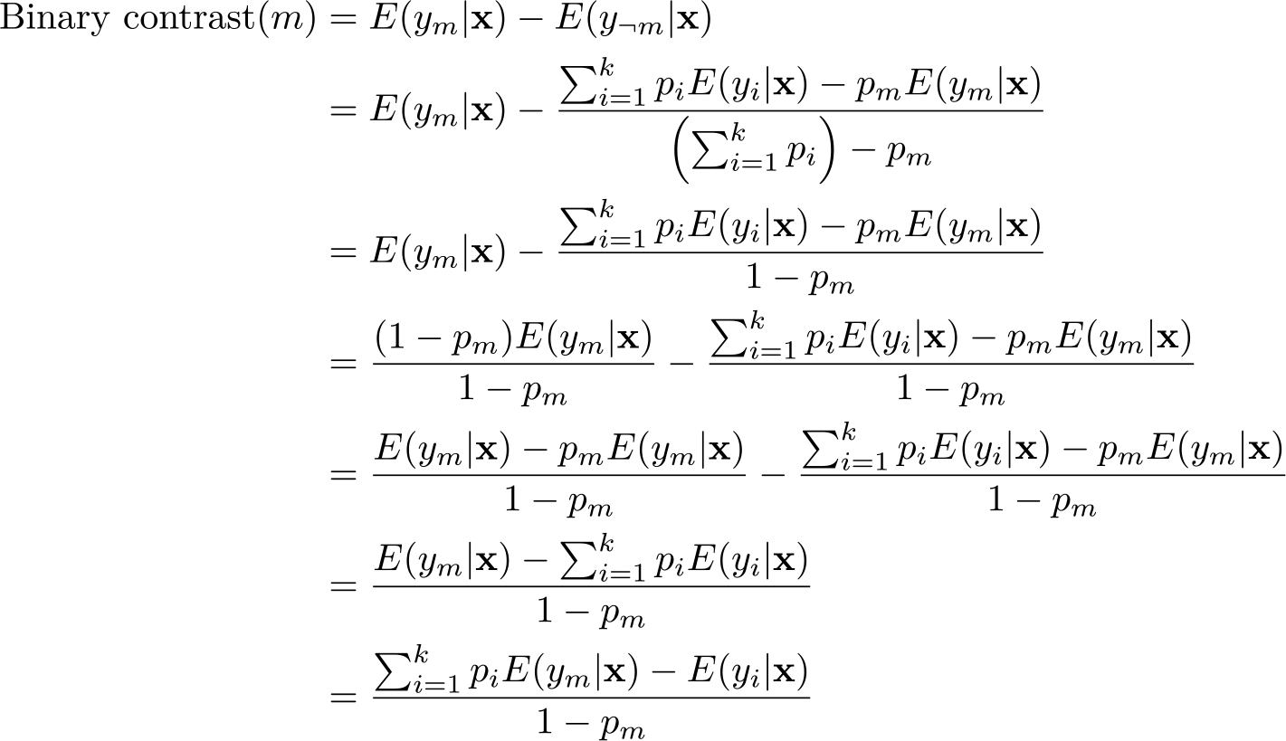
We arrive at a result for which, as written above, the only difference between the mean contrast and binary contrast is the denominator, meaning that

$\frac{\mathrm{Binary}\mathrm{contrast}(m)}{\text{ Mean contrast }(m)}=\frac{1}{1-p_m}$

The binary contrast can therefore be obtained from the mean contrast for the same category by multiplying the mean contrast by 1/(1 − p_m ). This implies that the mean and binary contrast for a given category will always be the same sign and that the coefficients and standard errors for binary contrasts are always larger than those of the mean contrasts. For a given category, the proportional increase in the coefficient and standard error is the same (a factor of 1/1 − p_m ), implying that the p-value for the test of the contrast versus zero is identical for the mean contrast and binary contrast.

binarycontrast uses Stata’s contrast command to automate the calculation of the binary contrast. Consider a regression model with polytomous regressor B that is specified with a reference category. We can use β_j for the estimated coefficient for the jth level of B, where β_j = 0 if the jth level of B is the reference category. We can specify a column vector β_B that contains [β ₁ …β_k ] for the k categories of B.

We can then transform β_B into various other contrasts of interest by specifying a contrast matrix C and computing C β_B . For example, mean contrasts are given by defining C as a k × k matrix in which

$C_{mn}=\{\begin{array}{ll}1-p_m\hfill & \text{ if }m=n\hfill \\ -p_n\hfill & \text{ if }m\ne n\hfill \end{array}$

where p_m is the (weighted) proportion of observations in category m. For the binary contrast, we change this to

$C_{mn}=\{\begin{array}{ll}1\hfill & \text{ if }m=n\hfill \\ -\frac{p_n}{1-p_m}\hfill & \text{ if }m\ne n\hfill \end{array}$

In Stata, the mean contrast as defined above can be computed using the contrast command and its gw. operator. contrast also allows the user to specify a custom contrast matrix. binarycontrast works by creating the custom contrast matrix and calling contrast. To construct the custom contrast matrix, binarycontrast requires the relative frequencies of the different categories, and it obtains these using Stata’s proportion command. When using proportion to obtain relative frequencies, binarycontrast uses the analytic sample and any weights that the user specified when fitting the model.

4 The binarycontrast command

4.1 Syntax

The command syntax is binarycontrast varlist [ , mcompare(method) mean eform [(name)] proportions] varlist includes variables for which one wants contrasts. While polytomous variables should be specified when fitting the model using factor-variable syntax (that is, i.region), one should not reuse factor-variable syntax with binarycontrast (that is, binarycontrast region).

4.2 Options

mcompare(method) provides the method for correcting for multiple comparisons. This is passed along to the contrast command when it does its calculation. See [R] contrast for details. The default is mcompare(noadjust).

mean computes mean contrasts instead of binary contrasts. The results are not different from using the contrast command directly.

eform (name) provides the exponentiated contrasts. If name is specified, it is used to name the column in the displayed results.

proportions provides a table with the proportions for each category in addition to the contrasts.

4.3 Stored results

binarycontrast stores the following in r():

5 Discussion

Although reference categories are the dominant way that coefficients for categorical regressors are presented, there is often little justification with unordered variables for prioritizing any particular category for interpretation. Basing interpretations on an arbitrary reference category may become increasingly strained for regressors with more categories. Both mean and binary contrasts provide coefficients for all categories that have a uniform interpretation, for which the sign of the coefficient corresponds with whether category membership is positively or negatively associated with the outcome.

The principal advantages of binary contrasts over mean contrasts are that the magnitude of the binary contrast for a category does not depend on the frequency of the category and that its basic interpretation is the same as the familiar way of interpreting a coefficient for a dichotomous regressor. Two disadvantages of the approach bear emphasis. First, for mean contrasts, the contrast between any pair of categories remains available as a matter of simple subtraction, but this is not the case for binary contrasts. Instead, one would need to multiply the binary contrast by the proportion in the category—that is, convert it to a mean contrast—to then be able to recover the contrast between a pair of categories. Second, while it is possible to extend binary contrasts to categorical interaction terms, the calculation is more cumbersome and the interpretation of the coefficient less clear, so binarycontrast does not include support for interaction terms.

6 Programs and supplemental materials

Supplemental Material, sj-zip-1-stj-10.1177_1536867X221083900 - Binary contrasts for unordered polytomous regressors

Supplemental Material, sj-zip-1-stj-10.1177_1536867X221083900 for Binary contrasts for unordered polytomous regressors by Jeremy Freese and Sasha Johfre in The Stata Journal