
Abstract
In this work, we describe the new command
1 Introduction
In this work, we present a command,
Traditionally, empirical analysis in economics has suffered from the scarcity of disaggregated sources of data (that is, at the level of individual, household, enterprise, etc.) such that, in the analysis of behaviors at the micro level, much was left to theoretical analysis. This situation oftentimes required heroically simplifying assumptions on the behavior of agents, the tradeoffs they were facing, and the absence of any path dependency, among other things. Nowadays, the ever-growing availability of disaggregated data on business firms has revealed a much richer picture than that previously conjectured based on theories alone or on aggregate industry-level data.
Firms are different along most of the dimensions typically taken into consideration by economic analyses. To provide a brief account of what is at stake, consider that even firms within the same, narrowly defined industry display very different levels of productivities, in terms of both labor and total factor productivities. 1 Also, the relative input intensities are much different (Dosi and Grazzi 2006), even with relatively similar input prices. At least as relevant, such heterogeneities are persistent over time; that is, if there is any selection at work, its effects take much longer to display (Dosi 2007). The ubiquitous presence of such heterogeneity has been vividly expressed by Griliches and Mairesse (1999): “We […] thought that one could reduce heterogeneity by going down from general mixtures as ‘total manufacturing’ to something more coherent, such as ‘petroleum refining’ or ‘the manufacture of cement’. But something like Mandelbrot’s fractal phenomenon seems to be at work here also: the observed variability-heterogeneity does not really decline as we cut our data finer and finer. There is a sense in which different bakeries are just as much different from each other as the steel industry is from the machinery industry.”
The evidence recalled above presents several challenges to the standard theory of production and to the related empirical applications based on the notion of a “representative” firm or an industry production function and, of course, on the estimation of such production function itself. The observed combinations of inputs chosen by firms appear to be quite dispersed, hardly displaying any regularity resembling a conventional isoquant. Further, although output—as expected—increases in both inputs, this does happen in a nonmonotonic way (Dosi and Grazzi 2006). In addition, the degree to which firms substitute their inputs is challenged by empirical observations.
Given all that, how can one obtain measures of productivity, at both the firm and the industry levels, that do not require assumptions not met by data, and on the contrary, that take into account such pervasive heterogeneity within the industry? In this article, we present a new application,
To illustrate heterogeneity and its relevance, we provide some empirical evidence in figure 1 that focuses on the labor productivity distribution, where labor productivity is defined as the ratio of deflated turnover value over number of employees. The details on these two variables can be found in section 4.1. 2

Empirical distribution of (log) labor productivity in a given 3-digit sector and two nested 4-digit sectors
In figure 1(a), the productivity distribution of a given 3-digit sector—that is, the solid line—is sufficiently widespread to indicate the huge productivity gap between the most productive firms and the least productive ones. On the graph, productivity is measured in a log scale, which makes the heterogeneity even greater. This heterogeneity does not disappear when focusing on similar firms (the firms with a 4-digit industrial classification, 3 that is, the dashed and dotted lines); we still observe significantly different productivity levels among firms. The persistence of heterogeneity indicates not only that heterogeneity holds when increasing the level of disaggregation but also that it holds over time.
As recalled above, not only do firms within the same industry display very different levels of efficiency, but also they employ very diverse production techniques. This is illustrated in figure 2.

Contour plots of adopted techniques and output in 3- and 4-digit sectors
Figure 2(a) provides a representation of production activities of firms within a given 3-digit industry 4 assuming the standard 2-input-1-output production, where the axes represent inputs (labor and capital are proxied by number of employees and fixed assets, respectively) and the contour line displays a constant level of output as proxied by turnover value. Thus, each firm within this industry, as one observation in our empirical data sample, can in principle be represented by one point in this contour plot.
In the input plane, we first plot all such points representing the firms’ labor and capital combinations from empirical data and then plot the isoquants indicating the possible combination of labor and capital corresponding to the same output level. As observed, dots in the input plane are quite dispersed while the corresponding isoquants do not display any regularity resembling a conventional production function. 5 Furthermore, the output increases with the inputs in a nonmonotonic manner. To be specific, given a quantity of one input, different firms attain the same level of output with very different levels of the other input. Again notice that this type of heterogeneity does not disappear when we increase the disaggregation of the industrial classification; similar phenomena can be observed in 4-digit-level industries, as reported in figure 2(b).
To sum up, this empirical evidence suggests that, within one industry, firms not only display very different levels of productivity but also have production techniques that are more heterogeneous. As a result, accounting for such apparent differences among firms would greatly improve productivity measurement and its change over time. In the next section, we focus on this attempt.
2 The zonotope approach to production analysis
In this section, we briefly outline the geometric approach to production analysis on which we rely for the proposed software packages. For a more detailed exposition, we refer the reader to Hildenbrand (1981) and Dosi et al. (2016).
The seminal work by Hildenbrand (1981) suggests an agnostic and data-oriented approach, which—instead of estimating some aggregate production function—offers a representation of the empirical production possibility set of an industry in the short run based on actual microdata. In such a setting, it is possible to represent a firm (or, for that matter, an establishment) in the input–output space. In such a way, the production possibility set of any given industry is represented geometrically by the space formed by the finite sum of all the line segments linking the origin and the points representing each production unit, called a zonotope. Based on this zonotope framework, Dosi et al. (2016) show that by further exploiting the properties of zonotopes, it is possible to obtain rigorous measures of heterogeneity and productivity without imposing on data a model like that implied by standard production functions.
Similarly to Koopmans (1977), Hildenbrand (1981), and now also Dosi et al. (2016), we denote the production activity, as representing the actual technique of production unit i, by a vector

which indicates that during the current period, this production unit, at its best, can produce αi
l
+1 units of output by means of

Further, with the assumption of N ≥ l + 1, Hildenbrand defines the short-run total production set associated with the family {

of line segments generated by production activities {

Hildenbrand also defines his short-run efficient industry production function within the zonotope framework. Let’s project the above-defined zonotope

Thus his production function F :

This definition implies that, given the level u 1 ,…, ul of inputs for the industry, the maximum total output could be achieved by allocating, without any restrictions, the amounts u 1 ,…, ul of inputs over the individual production units within the industry in one of the most efficient ways. However, the frontier associated with this production function does not provide any information on the actual technological setup of the whole industry. This production function could not be the focal reference either, from a positive or from a normative point of view (Hildenbrand 1981).
Within the zonotope framework, Dosi et al. (2016) define the main diagonal of a zonotope

Obviously, if all firms in one industry were to use the same technique in a given year, all the vector-firms would lie on the same line. This is the case where only one technology is adopted and all the firms within this industry are homogeneous. In this case, the associated zonotope would degenerate to one with null volume, that is, coinciding with the diagonal
First, let

where

where
Aside from the heterogeneity measure, Dosi et al. (2016) also suggest that the angle formed by the industry production activity vector

where for any vector
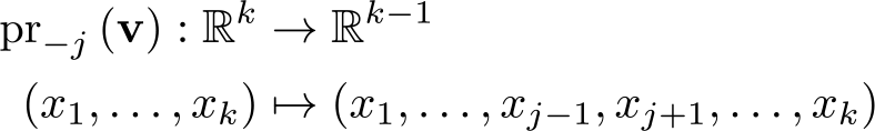
Θ
j
(
A few remarks are needed on the nature of the measure, its relation to similar techniques, and the scope of applicability. Notice that the volume of zonotope, as well as the angles, are measures and not estimates. Further, although the measure of productivity bears some similarity, mostly because of the nonparametric nature, with data envelopment analysis in production (see, among others, Farrell [1957], Charnes, Cooper, and Rhodes [1978], and Simar and Zelenyuk [2011]), the two methods are clearly distinct; the zonotope approach considers all firms, not just those on the frontier. Although both approaches are data driven and nonparametric, the emphasis of data envelopment analysis is, for the industry, to construct the efficient frontier by enveloping the data and, for the individual firm, to proxy its efficiency (for an application to Stata, see Ji and Lee [2010] and Badunenko and Mozharovskyi [2016]). Empirically, the traditional deterministic approach faces some issues, which have been addressed by recent work. To be specific, Daraio and Simar (2007) deal with the sensitivity to measurement errors and outliers, and Cazals, Florens, and Simar (2002) and Daraio and Simar (2005) propose robust frontiers. In addition, there exists a command that deals with such issues; see Belotti et al. (2013).
As recalled above, the zonotope approach provides a general framework not necessarily limited to industry heterogeneity and productivity analysis. For example, Aruka (2017) argues that the zonotope framework provides a different view of the production set and discloses new possibilities for modeling international trade. In the latter field, he suggests a further generalization of the model so that it is possible to jointly assess more than three countries and three commodities, thus abandoning the limiting special case of two countries and two commodities. In a rather different domain, the software application we are presenting here can be used to compute measures of multivariate disparity similar to those outlined in Koshevoy and Mosler (1996, 1997).
In sum, the proposed framework allows the investigation of the production and productivity dynamics of firms while taking into consideration the existing heterogeneity across firms, which is high and persistent even within the same industry. The geometrybased approach, on one side, enables us to relax many of the current existing assumptions, which have often been shown to lack empirical support. On the other side, while it allows for providing a representation in the production space with several inputs and outputs, on two or three dimensions, it is a way to provide an illustration of the trend of the industry and of individual firms.
To reinforce the last point, we take advantage of the simple one-input, one-output setting, as depicted in figure 3.

One-input, one-output examples of zonotopes
There are two firms, represented by
We conclude the section with table 1, which summarizes the key concepts of the proposed zonotope method.
Key concepts of the proposed method

3 The zonotope command
In this section, we introduce the command
3.1 Syntax
The syntax of the command to compute the zonotope is
where the option
3.2 Description
The
3.2.1 Output and return value
The
When the
All the scalars returned by
and the elapsed time can be displayed with
3.2.2 Output vector: diagonal
The output vector

Clearly, it is an (l + 1)-dimensional (row) vector. It can be easily displayed on screen (or reused) using
3.2.3 Output vector: tangents
The output vector
3.2.4 Output matrix: gen
The output matrix
We report below a brief description of the eight statistics mentioned above. Some of them have a clear economic interpretation because they directly correspond to the key concepts of the proposed method, while others are necessary intermediate steps toward the measure of interest.
Statistic S1: Volume
Given N generators

where Vol(·) follows (3). We report this volume as
Statistic S2: Diagonal’s norm
The norm of the diagonal ||

The length of the diagonal of the zonotope represents the “size” of the industry; the longer this vector, the bigger the industry is.
Statistic S3: Sum of squared norms of all the generators
As indicated by the name, we first compute for each generator the sum of the square of each of its components, and then we sum over all generators.

Statistic S4: Gini index
According to (4), this Gini index is computed as the ratio between the volume of the zonotope and the product of the components of the diagonal. We rewrite this industry heterogeneity measure as follows:
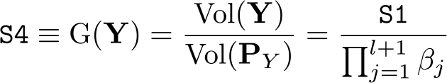
where
Statistic S5: Tangent of angle formed by diagonal and input space
Given the diagonal vector reported as

Intuitively, it provides our measure for industry productivity. In a two-inputs, one-output setting, the “steeper” the vector, the more productive is the industry.
Statistic S6: Cosine against output
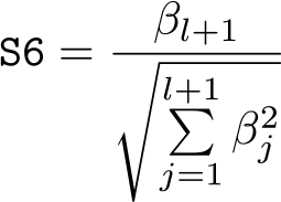
Because of the complementary angle relationship,

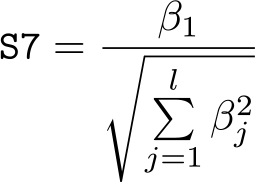
Statistic S7: Cosine of diagonal projected on input plane with x axis
The angle formed by the x axis and the projection of the diagonal in the input plane measures the relative intensity of the first input related to the other inputs. We report its cosine value as
Statistic S8: Volume against cube of the norm of the diagonal
The last statistic is the ratio between the volume of the zonotope and the cube of the norm of the diagonal.

This definition of volume is restricted to the boundary edges of the cone of all possible vectors, and as such, it considers only the most diverse vectors. It attempts to measure the maximal diversity of the field (hence, it takes into account only the boundary vertices) by measuring how “wide” the cone is.
Other than these statistics, the command also provides the elapsed time, expressed in minutes.
3.3 A working example of the zonotope command
In this section, we provide a step-by-step working example that shows the use of the
We start by loading the dataset into Stata and listing the first five rows:

The first column indicates the year, and the second reports the firm’s sector of main activity. Columns 3 to 6 report, respectively, number of employees, fixed assets, material cost, and turnover. The last column prints a fake ID of the firm. In the interest of replicability, we are providing artificially generated data that display the same distributional properties as the “real” data used in other works, such as Dosi et al. (2016) and Dosi et al. (2021). Each row in the dataset represents a different firm in a given year and industry.
As usual in the literature, the number of employees and fixed assets are used as proxies for labor and capital inputs, respectively, and turnover is used for output. In this two-inputs, one-output setting, the

We will go through the results step by step to provide specific comments about the results relevant to the investigation.

The above, the first part of the output, after informing us about the version of the package, displays the number of dimensions of the current analysis (3 in the example) and the number of generators that in this case are firms (160).

The second part of the output, shown above, reports the production activity of the whole industry, the diagonal of the zonotope, as defined by (2), which is the result of the aggregation of the 160 generator-firms. The total number of employees in this industry is 5,531, while the total fixed assets and turnover of this industry are equal to 459,015 and 2,846,360 thousand Euros, respectively.

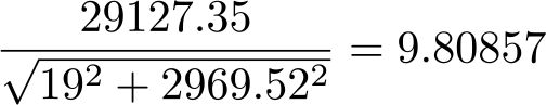
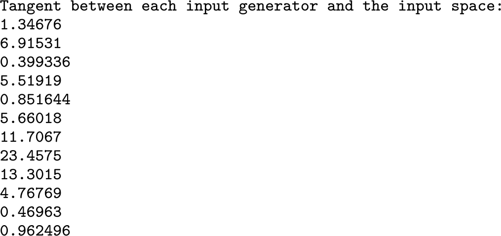
For the sake of exposition, we reported only the tangent for the first five firms of this example. As will be discussed in section 4.2, we extend the definition of industry productivity, (5), to individual firm productivity, as proxied by the angle that the vector-firm forms with the input plane. For example, firm 145725 produces 29,127.35 thousand Euros of output from 19 employees and 2,969.52 thousand Euros of fixed assets. According to (6), productivity of firm 145725, as proxied by the tangent of the above-mentioned angle, is
Recall that a higher value of the tangent of the angle suggests a higher productivity because the vector-firm is steeper; that is, the angle that the vector forms with the input plane is larger. Figure 3 provides a simple illustration of this, in a one-input, one-output setting.
As for many other indicators of efficiency that use multiple inputs, the value of the measure alone is not of great use. It is much more relevant instead to perform a comparison across firms within the same industry or an intertemporal comparison of the same unit over time. This is the sort of comparison that is proposed in table 2 in section 4.1.

As shown above, the
The
The last bit of output is displayed as follows:
This is the computation time. As we will explain more in section 5, building the zonotope of a set of generators has an exponential complexity (that is, it is very time consuming, especially in a high dimension and when the number of generators is high).
It is possible to display (or reuse) the computed results as follows:

4 Empirical analysis
In this section, we provide three additional, more-advanced examples of using
4.1 Assessing industry heterogeneity
In this section, we conduct some empirical investigations on industry heterogeneity and productivity. We do this by using larger sets of data to replicate the standard situation faced during empirical analysis on firm-level data, where firms are grouped according to their sector of main activity, at different levels of aggregation.
For replication of all the analyses, we use the same data introduced in the previous section. For each firm in the selected industries, number of employees and fixed assets are chosen to proxy inputs and turnover is chosen for output. All values except for the number of employees are assumed to be in thousands of Euros and deflated at the 4- digit
4.1.1 The two-inputs, one-output case
Traditionally, the most standard setting in which to investigate production is that which assumes production activity with two inputs and one output; number of employees and fixed assets are chosen to be the proxies for inputs and turnover value is chosen for the output. For each industry in one specific year, the normalized zonotope volume and the tangent value of the angle formed by the industry production vector and its input plane are easily computed as

From the available results, we select

Computation results for Gini coefficient and productivity among selected sectors and years—ℝ 3 case
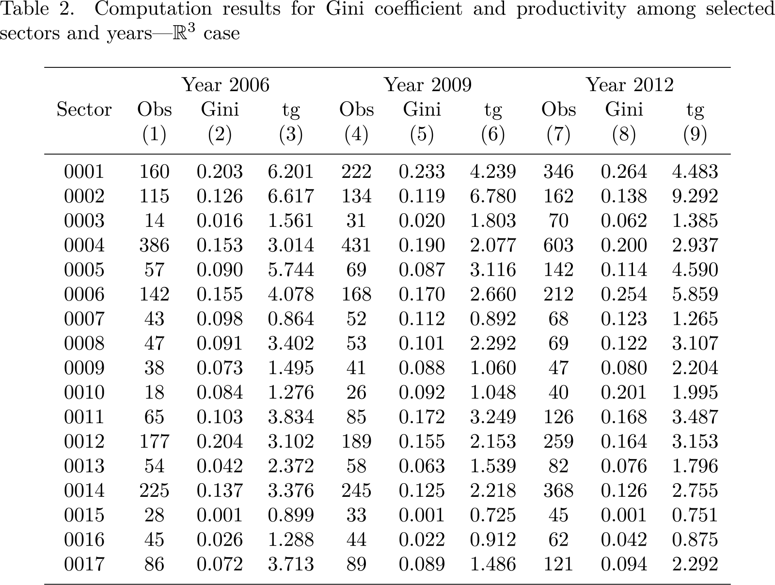
The chosen normalization strategy for the volume of the zonotope seems to be effective, because there is no apparent relation between the number of generator-firms and the Gini coefficients. For example, in 2006, there are 386 firms in sector 0004 and 160 firms in sector 0001. However, given the larger number of firms in sector 0004, we do not necessarily expect its Gini coefficient (the normalized volume of the zonotope) to be bigger than that of sector 0001. Indeed, based on our data sample, the Gini coefficient of sector 0001 is larger: 0.203 compared with 0.153 for sector 0004.
After taking into account the effect due to the number of firms, we notice that the heterogeneity levels are different among different industries. For example, in 2006, the Gini coefficients vary from 0.001 for sector 0015 to 0.204 for sector 0012. Similarly, as indicated in column (3), the productivity levels among different sectors are different.
From columns (4) to (6) and from columns (7) to (9), we report similar results in the years 2009 and 2012, respectively. This allows us to explore the dynamic of industry heterogeneity and productivity over time. Most of the selected sectors share an upward trend in their heterogeneity levels. For example, the heterogeneity level of sector 0001 increases from 0.203 in 2006 to 0.233 in 2009, and again to 0.264 in 2012. As for the productivity, for most of the industries, we report a decrease from 2006 to 2009 and an increase from 2009 to 2012.
The same analysis can be performed in the case of four dimensions, for instance in the three-inputs, one-output case. 10 In the interest of space, results are not reported here, but they can be obtained with the following commands:

4.2 A geometric approach to firm-level productivity
As indicated in (5), Dosi et al. (2016) propose as a measure for industry productivity the tangent of the angle formed by the industry production activity vector

The

Among the available results, we focus on that referring to firm productivity:
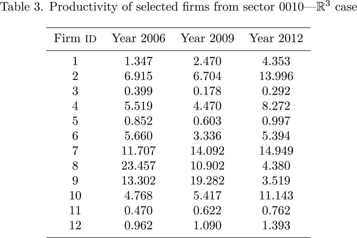
We then compute productivity of these firms in 2009 and 2012 and report the results in the respective columns of table 3. Note that, in accordance with previous findings, firm-level productivity displays persistence, and hence the large within-industry dispersion does not vanish over time.
Productivity of selected firms from sector 0010—R3 case
4.3 An application to inequality
The
4.3.1 Introduction to multivariate Gini coefficient
Following Mosler (1994) and Koshevoy and Mosler (1996), we focus on two multivariate Gini coefficients. To do this, we denote by

for i = 1,…, N. Correspondingly,

indicates the share of attribute j out of the total amount owned by unit i. Vectors

for i = 1,…, N.
Mosler (1994) introduces a multivariate Gini index by using the volume of the Lorenz zonotope (LZ) as the Minkowski sum

of line segments generated by
where zonotopes are defined as the Minkowski sum

of line segments generated by vectors
To show the necessity of resorting to this further measure, we use a toy example detailed in appendix A. We focus on x and z, representing two attributes among the 10 units. Using the
To get this volume-Gini index, we need to use the
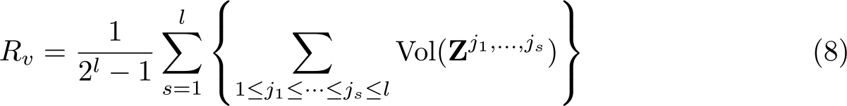
4.3.2 Empirical application of multivariate Gini coefficient
We present an empirical exercise based on actual data from the Namibia Household Income and Expenditure Survey 2009/2010 (The Namibia Statistics Agency 2013). 13 This dataset includes detailed information about income and expenditures of 9,643 households in Namibia from 2009 to 2010. For each household, we compute the income per capita (IPC) and expenditure per capita (EPC) based on the income, expenditure, and number of people in the household. 14 Notice, in particular, that the survey reports only the main source of income for each household. As a result, we have two attributes of each household, IPC and EPC, either of which can be used for computing the traditional univariate Gini coefficient.
In many studies, the univariate Gini coefficient based on IPC is adopted as the measure of inequality. We report it at the bottom of column (1) of table 4. Correspondingly, the univariate Gini coefficient based on EPC is reported at the bottom of column (2). The univariate Gini coefficient indicates a higher inequality level based on expenditure (0.780) than income (0.611). As we discuss above, these two attributes can be taken into account simultaneously by computing the volume of the corresponding LZ and multivariate volume–Gini index. We report them at the bottom of columns (3) and (4), respectively. It is not possible to compare the values of the univariate and multivariate Gini indices, because they are constructed in different ways. 15 However, it is meaningful to compare one of the indexes cross-section or over time.
Various Gini coefficients among households with different income sources in Namibia from 2009 to 2010

Let us conduct a cross-section analysis now. Households are classified into seven groups according to their main source of income. We report the univariate and multivariate Gini coefficients between columns (1)–(4) in table 4 and the number of households per group in column (5). Notice that groups with different income sources display different inequality levels. According to the univariate Gini coefficient based on IPC, the least unequal group is the one relying on state old pension. This seems reasonable because state old pensions, compared with other sources, are expected to be more equally distributed among receivers.
The next thing to notice is related to the potential bias associated with Vol(
We provide the code to generate the fourth row of table 4. First, we generate the relevant variables, that is, IPC and EPC, from the raw data.
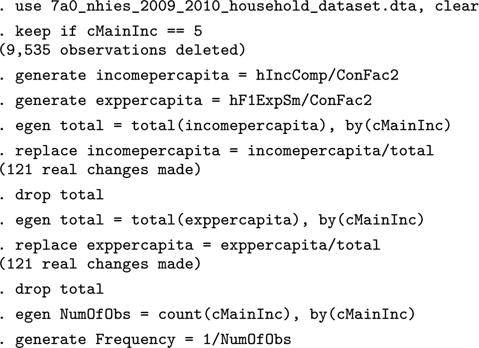
Then, we compute the univariate Gini coefficient based on IPC and EPC by using the community-contributed command

Finally, we compute Vol(

5 Analysis of zonotope computing time
Computing the volume of the zonotope given the list of its generators can potentially be time consuming, because its computational complexity is O(Nl ), where N is the number of generators and (l + 1) is the dimension of each generator (that is, its length). Thus, this algorithm falls within the exponential category; that is, its time does not scale in a polynomial way but in an exponential way. In particular, when N is kept constant, it is clearly exponential in the number of dimensions (l + 1).
Table 5.provides the elapsed times for a varying number of variables (from 2 to 6) and a fixed number of generators (N = 200). On the contrary, table 6 provides the elapsed times for a varying number of generators (from 50 to 250) and a fixed number of variables [(l + 1) = 6]. We ran the experiments on an Intel CPU i7 4-cores on a Windows 7 operating system, with 32 GB of RAM using Stata/IC. The data from tables 5 and 6 are charted on figures 4 and 5, respectively. From these figures, we can clearly see how the time complexity of computing the volume of the zonotope is exponential. To empirically prove that the time complexity is Nl , we have plotted in figure 6 the fifth root of the elapsed times, when the number of variables (l + 1) is equal to 6. The fact that the graph is a perfect straight line proves that the dependency is a power of 5, as expected.
Elapsed times for varying numbers of variables and 200 generators

Elapsed times for varying numbers of generators and 6 variables


Elapsed time as a function of the number of variables, for 200 generators

Elapsed time as a function of the number of generators, for 6 variables

The fifth root of the elapsed time as a function of the number of variables, for 6 variables. The fact that the graph is a perfect straight line empirically proves that the computational complexity is Nl , because (l + 1) = 6 in our case (N = 200, of course).
6 Conclusions and future work
The recent and increasing availability of disaggregated economic data challenges many of the standard theoretical assumptions, yet there is still urgent need for adequate tools to deal with these emerging rich and complex empirical observations.
The
The software package we introduced is ready for applications in other domains; the zonotope framework itself is already used in other fields, for example, still within economic analysis, to assess inequality.
8 Program and supplemental materials
Supplemental Material, sj-zip-1-stj-10.1177_1536867X221083854 - A toolbox for measuring heterogeneity and efficiency using zonotopes
Supplemental Material, sj-zip-1-stj-10.1177_1536867X221083854 for A toolbox for measuring heterogeneity and efficiency using zonotopes by Marco Cococcioni, Marco Grazzi, Le Li and Federico Ponchio in The Stata Journal
Footnotes
7 Acknowledgments
We gratefully acknowledge Gianluigi Tiesi (Netfarm s.r.l.) for support in creating the git repository and help in generating the Stata plugin. This project has received financial support from the European Union’s Horizon 2020 research and innovation program under grant agreement No. 649186—ISIGrowth. This article was presented at the 2019 Italian Stata Users Group meeting in Florence. We thank the participants at the conference for their comments. Suggestions and comments by an anonymous referee were much appreciated. The usual caveat applies. Le Li is the corresponding author.
8 Program and supplemental materials
To install a snapshot of the corresponding software files as they existed at the time of publication of this article, type
To update the
To run the demo, execute the following do-file:
If the demo runs correctly, you are done.
However, it may fail, especially if you are using an operating system for which the plugin has not been generated yet.
In this case, the plugin must be generated from scratch, as explained next.
8.1 How to generate the zonotope plugin
It contains everything needed to generate the Stata plugin for most platforms (see below).
To generate the plugin, the following things are required:
a C++ compiler the CMake utility (optional) the GIT utility (it is useful for downloading the tree of the whole project or specific subprojects)
The CMake utility is required to compile the plugin as a shared library. This shared library, named
The ado-file is named ![]()
The plugin generation has been tested on Windows 10 64-bit using Visual Studio 15, on Linux Ubuntu 18.04 64-bit using GCC, and on Mac OS 10.12.3 (16D32) 64-bit using the Mac OS Sierra operating system, with LLVM C++ compiler.
If you have troubles with the plugin, please open an issue on the associated GitHub repository. We will do our best to help you.
Notes
A A simple toy example
As a simple example, we enter the following commands:
We now have the following dataset loaded into Stata memory:
The dataset contains only 10 observations and 3 variables:
We now enter the following command:
This command builds the zonotope on input variables
The following result will be displayed:
As is explained in greater detail in section 5, building the zonotope of a set of generators has an exponential complexity (that is, it is very time consuming, especially in a high dimension and when the number of generators is high). Therefore, we decided to implement it in C++, to reduce the run time as much as possible. In section 8, we provide step-by-step instructions for compiling the C++ source code to create the plugin (a binary file with extension
References
Supplementary Material
Please find the following supplemental material available below.
For Open Access articles published under a Creative Commons License, all supplemental material carries the same license as the article it is associated with.
For non-Open Access articles published, all supplemental material carries a non-exclusive license, and permission requests for re-use of supplemental material or any part of supplemental material shall be sent directly to the copyright owner as specified in the copyright notice associated with the article.