Speaking Stata: Loops in parallel

Abstract

This column is a tutorial discussing looping in parallel using foreach and forvalues. Such looping may use not only local macros defined for the purpose but also other devices, including the gettoken command and ways to increment and decrement other macros and to evaluate other expressions.

The main idea is that a set of loops in parallel is essentially one loop with two or more sets of parallel actions. Examples cover looping over integers with a required specific display format, generating new variables and defining variable labels at the same time, binning variables as desired, and putting skewness results in new variables. The last example includes some historical comments on the tangled literature on skewness measures using medians and quantiles.

1 Introduction

In many Stata problems, you want to do (almost) the same thing again and again. You want to work your way through a list, looping over the items in that list. Often, Stata does this for you. Automatic looping over observations for many operations comes as a surprise to users who have become accustomed to spelling out such loops in other software. But at other times, you have to ask Stata to do it for you. The concern here is with the tools provided for that purpose and specifically with how you can best work your way through parallel lists using loops.

foreach and forvalues, introduced in Stata 7, are the main workhorses for looping through lists. If these are new to you, then apart from the online help, first see [P] foreach and [P] forvalues or my earlier tutorial, which included key guidance on local macros (Cox 2020). These references to the Programming Reference Manual do not mean that you have to write Stata programs to be able to use these constructs. On the contrary, they are often used interactively, or you can incorporate them in do-files or code you run from the Do-file Editor.

To clarify if it is obscure: What is a Stata program? Strictly, whatever is defined by a Stata program command. Note that this definition is not circular, because a question in one language (a discussion of Stata) is answered in another language (Stata itself). However, we will not be writing any Stata programs in this column. More loosely, a Stata program is any set of Stata commands, for example, in an interactive session or a do-file or the contents of a Do-file Editor window. So as soon as you typed your first Stata command or even selected a command using the menu, you started out as a Stata programmer.

This column is essentially a replacement for Cox (2003). Only some of the original text remains. That column had much discussion of how such problems were handled in the now undocumented for command, which is now likely to be of little or no interest to most readers. The column remains accessible otherwise. Other developments in Stata from Stata 7 onward and greater personal experience have led to some different emphases and examples. In particular, the first extended example in the 2003 column was a riff on various ways to rename a set of variables, a riff long since made obsolete by extensions to that command in Stata 12.

2 Warm-up: Looping including leading zeros

As a warm-up, let’s look at an example so mild that you might not even think of it as a problem in parallel looping. You want to loop over 00 through 09 and through 10 through 20 as two-digit identifiers. For example, you might be concerned with years from 2000 on. The need could be for data import: many people use filenames with such prefixes or suffixes, perhaps mindful of how those filenames sort. Or the need might be for some kind of display, however defined.

Spelling out the 21 labels is not attractive, and we know how to loop over integers 0 to 20, but how do we get the leading zero in some cases but not all? One answer (Cox 2010b) is to push the integers through a display format. As a test of the code, we could write down a first loop such as

Once that is working, we want to do something that might lead us to put the result in a new local macro, say,

We would then develop the code to do what we want to do, such as manipulate filenames or whatever else.

This small example is the idea of loops in parallel in a nutshell. We loop over integers 0 to 20, with a parallel action that adds a leading zero when it is needed. (If you are finding this very tame, consider how extra digits such as 81 to 99 could be added.)

3 Problem: New variables with new variable labels

3.1 The problem stated

Here now is a slightly more challenging example. None of the examples here will get very long, so the tutorial understates the extent to which looping can clarify and condense realistic code. We must start with simple examples, as you will appreciate.

Suppose you want some powers of a numeric variable in new variables. To have it both ways, you want concise variable names as well as informative variable labels. Given a numeric variable x, then some powers are, say,

which would yield xp2, xp3, and xp4 as containing the square, cube, and fourth power of x, respectively. Assigning variable labels as well could be done one at a time, but doing that within the loop should seem attractive. Precisely how to do that will be the topic in a later section.

The most important idea, once again, is simple. Loops in parallel do not imply any special construct in Stata. They are just generally one loop with actions in parallel. Some other commands that may be new to you turn out to be especially handy, but those are the only details needed.

The principle is now out in the open. There are many tricks available in practice. The choice between them is partly one of taste and partly one of circumstance.

Again starting out very simply, let’s suppose for the moment that our desired variable labels for xp2, xp3, and xp4 are, respectively, quadratic, cubic, and quartic. If your reaction is that these are not especially good variable labels or that these would do fine as variable names, please hold on because your reaction will find an answer shortly.

3.2 A few words on words in Stata

At this point, a simplifying detail is that these intended variable labels are all single words. A first stab at Stata’s definition of a word is that words are separated by spaces. That is, “word” has a technical sense in Stata that is only loosely related to grammar in English or any other language. In your Stata practice, you are not restricted to variable labels that are single words, and you should already have seen (and likely have defined yourself) many variable labels that are more complicated, which is most of the point.

This definition has some simple consequences. In particular, if presented with the string "1 2 3", Stata sees there three words; the fact that these words imply numbers is consistent with Stata’s definition of words.

More will be said about words in Stata, to come when we need to know about it.

4 gettoken is your friend

4.1 gettoken can produce a parallel action

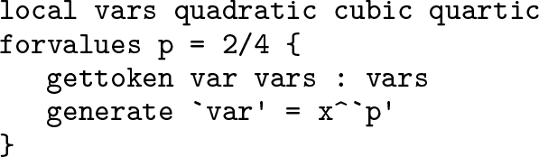
Even for this very simple problem, Stata offers several solutions. I first focus on using gettoken, which is my preferred approach for lists in parallel. Code first; comments follow.

In this approach, we first put the labels in a local macro, labels. Each time around the loop, gettoken takes the first word in that local labels and puts it in a different local macro, label, and the remainder of the macro content back into labels. The macro names, here labels and label, are yours to assign, but in your own code, do choose names that make the distinction clear to you.

Note that the syntax is to be read from right to left: the input labels is to be split into 1) all but the first item back into labels and 2) the first item into label.

Many people like to think of the local as here defining a stack, like a (tidy) stack of papers or books. Each time round the loop, we take the top item (here a word) off the stack and use it. Next time round, the stack has one fewer item.

Let’s make that concrete. The first time around the loop, quadratic is taken off the stack and used as the variable label for xp2. So cubic and quartic remain on the stack. The next time around, cubic is taken off the stack and used as a variable label for xp3. quartic remains on the stack and will be used the last time around the loop for xp4.

So that is the main idea in miniature. We have there two loops in parallel. We loop over the integers 2, 3, and 4 as powers we need to use for calculation and to use within new variable names. At the same time, we use gettoken to loop over words to be used as variable labels.

4.2 A few token comments

The command name gettoken hints at an idea of tokens, so what are tokens to Stata? Loosely, but sufficiently for now, any character string can be split into tokens or sub-strings, and a token is defined by whatever is used to split the string. By default, and very commonly, spaces are used to split (or parse) strings, and then the tokens are words. But Stata users, and so programmers too, can employ various kinds of tokens. For example, lists often arrive with items separated by commas, and there are many other possibilities—the parsing characters do not have to be of just one kind. In short, the idea of tokens is much more general than that of words.

A glance at the Stata help for gettoken and the associated manual entry [P] gettoken indicates many uses for the command, especially for programmers parsing user input to their own programs defining new commands. In contrast, its use here for loops is essentially implicit in that manual entry.

4.3 Back to the problem

The example is simple enough to get right quite easily. We defined three tokens (just words) to be used as variable labels for three variables. In practice, the syntax is forgiving, although you may not always think that to be a feature whenever it bites you. First off, gettoken is not even aware that it is inside a loop. It does no checking to see whether you have the right number of tokens for your purpose. If the stack contains more tokens than you need, superfluous tokens will never be used. If the stack contains fewer tokens than you need, an empty string will be used instead. Whether that is a problem depends on what you are trying to do. Here assigning an empty string as a variable label is perfectly legal, even if it is not what you want. In other problems, the empty string might make a command illegal as well as inappropriate.

But note especially that this approach is destructive. If it works as intended, you will consume most if not all of the macro contents, so watch out.

Let me now redeem some promises. We need to revisit the suggestion that the words offered would be fine as variable names. We can now apply what has been learned:

Evidently, I changed the local macro names, which is a good idea although not essential. Often, programmers amuse themselves by using facetious or even rude names. I am all in favor of programmers being amused, but watch out in code that will be read by others. Ideally, that means all your code, because you should want your research to be transparent, at least to your intended readership. Serious advice is to think up your own conventions and stick by them. That could be especially helpful if you are a member of a team reading and changing code together. In the example so far, p is intended to suggest “power”; names that are evocative are always worthwhile. Common or at least possible conventions for macro names that serve as loop macros include i or j for anything suggesting rows or columns, v for variable, g for group, t for time, and so on. Avoid the letter l, which is all too close visually to the numeral 1 (one).

We need to revisit also the question of wanting different variable labels. Someone might insist that (say) x ² is a square whereas (say) b ₀ + b ₁ x + b ₂ x ² is a quadratic, so better variable labels might be, in turn, square, cube, and fourth power. Note the deliberate but utterly realistic complication: fourth power is a string with two words.

If you have one foot firmly in the history of mathematics, then you might be happy with biquadrate for the fourth power (Schwartzman 1994; Lo Bello 2013). Otherwise, I guess not.

Our examples so far have leaned on the simple fact that we were dealing with single words only. Again, as the name gettoken implies, the general currency here is tokens, which evidently may be single words. But as already hinted, the definition of a word in Stata can be more complicated. Although words are separated by spaces, it is also considered that double quotes (" ") and compound double quotes (`" "') bind more tightly than spaces separate. So we need to flag that "fourth power" is one word in this extended sense and thereby also one token. In practice, it is a good idea to put the entire set in compound double quotes. That done, the rest of the code carries over.

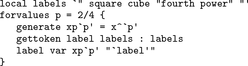
We now know about enough machinery to extend code to other problems. Suppose we want three things at once:

1. powers 2, 3, and 4 as before;

2. names like xsq, xcu, and xqu because we are looking forward to being able to call them up as a team through a wildcard, x??; and

3. variable labels as just given.

This is more complicated but not fundamentally different. We have one loop only with three lists to deal with in parallel. Here is one way to do it:

At this point, if not earlier, you may be thinking that you could just write down three statements to generate each variable and at most three more statements to define variable labels if you want them also. So is this a lot of fuss that—for the problem stated—makes clear and concise code more unclear and possibly even more verbose? For simple examples, the point is good, but nevertheless the machinery is invaluable for lists with many more items.

5 Using macros as counters

5.1 Other methods use counters more

We could have written those loops differently. Other methods to loop in parallel typically hinge more on using macros to count our way around the loop.

Consider this way to do the last loop:

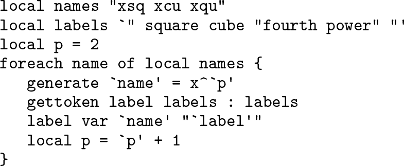
Done this way, we take over the manipulation of local macro p ourselves, which implies responsibility both for initializing the macro by setting it to 2 before we enter the loop and for incrementing the macro each time around the loop. So after the first new variable, xp2 is generated as the square of x and assigned a variable label. Then we can increment p. And so on, similarly, for each time around the loop.

Increment is an old English word and more general in meaning, but in a programming context it often connotes precisely incrementing by 1, or adding 1. If the code says otherwise, that settles the matter. “Bump up” is more informal, but the same applies: “bump up” with nothing else said means bump up by 1. Again, if programmer comment or conversation says differently, then the meaning changes accordingly. The same goes for decrement, meaning subtracting, and for the more informal “bump down”.

5.2 The operators ++ and − −

This operation of incrementing an integer held in a local macro is so often needed that Stata allows a different syntax, one common in many other languages.

local ++p

always is equivalent to

local p = `p’ + 1

Indeed, you can refer to `++p', which increments on the fly. So this is an alternative to the previous loop:

Hence, we initialize the local macro p to 1, but each time around the loop the macro is incremented by the ++ syntax. So we can remove the line that increments the local by 1. If other computing experience has made such syntax familiar, well and good, and you may even have been missing it. Either way, let’s go through that again.

In our example, we lost a line and gained a reference to `++p', which is one of a set of quadruplets. Seen all at once, with our example macro name p, they are `p++', `++p', `p--', and `--p'. In context, Stata sees `p' and knows that this means to “evaluate the local macro p and then put its contents here” as part of parsing a command that is then executed (if legal). What we have now with `++p' is threefold:

1. Evaluate the local macro p.

2. Add 1 to the value of the macro.

3. Put its contents here.

So if before Stata reads this, p evaluated to 1, then after Stata reads this, it will evaluate to 2. The incrementation is performed in place.

The other quadruplets are all similar. `i++' increments after use, `i--' decrements after use, and `--i' decrements before use. Double characters (++ and --) represent single operators. The key to learning their meaning is just to take the left-to-right order of macro name and operator literally. What comes first is done first.

What is more, these operators apply only to local macros and nothing else. After global i = 1, display $i++ is illegal. display "$i++" is perfectly legal but does nothing special: you just get shown 1++, which might even be something you want to print. But on reflection, you will see that this restriction is no restriction because once you can do it with local macros, you can indirectly do it with other objects.

Nevertheless, watch out:

local p++

is legal in Stata, but it is nothing to do with incrementation. An early decision in Stata was not to insist that a space must follow a macro name in a macro definition. That being so, that definition assigns the string ++ to the macro p. When ++ as a prefix was allowed, it was decided not to reverse that, considering all the programs and do-files that such a change might have broken.

If this syntax is entirely new at this point, you may think it cryptic or rather too clever. But nevertheless, at some point you are likely to change your mind and start using it.

5.3 The word # of syntax

There are other ways to use counters. Something like this is often done:

The word # of syntax extracts a particular word from the string given. Given the macro name, Stata evaluates it before the statement is executed. That is, the first time around the loop, Stata sees

local label : word `p’ of `labels'

and immediately translates it as

local label : word 1 of square cube "fourth power"

and then executes the command. More generally, Stata tries to execute a command because a command that is illegal will trigger an error message. That is backward because whatever triggers an error message is what we call illegal.

So that syntax avoids the use of gettoken if you have yet to regard it in a friendly manner. But notice how problems quite easy to explain can still be a little tricky. We want the first label to go with the variable containing power 2 and similarly the second and third labels to go with the powers 3 and 4. There is an offset between the powers 2 3 4 and the words 1 2 3 that we want. Here a good solution is just to make sure that we extract the word before we bump up the local macro p. Small devices like that are often enough. In yet other problems, it may be cleaner and clearer to have two or more macros as counters, separately maintained, even if the problem calls for parallel loops.

This word # of syntax is just one of many helpful tools whose documentation starts with the help for [P] macro.

5.4 tokenize

To show that in action, we will use it in the next example, which also draws into the discussion the command tokenize. Even if you have not seen that command before, its name should suggest its job, to split a string into tokens. What it does beyond that is assign the tokens to local macros with names that start at 1 and continue with 2 and so on.

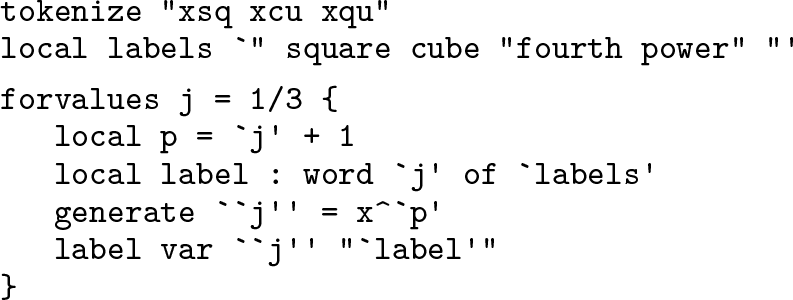
In that code, the tokens xsq, xcu, and xqu are thus mapped to local macros named 1, 2, and 3. We later use those macros in the nested reference ``j’'.

tokenize is yet another command from Stata programming that can be used interactively; see [P] tokenize. It takes its argument, splits it into tokens, and assigns those tokens to local macros 1 and up according to how many tokens there are. By default, tokens are just words in the Stata sense used earlier. As already pointed out, they are more general than words because they can be delimited by something other than spaces.

In this example, after tokenize, local macro 1 will contain "xsq", local macro 2 will contain "xcu", and local macro 3 will contain "xqu". The effect of tokenize is here equivalent to three statements:

which you should prefer only if you are paid according to the number of lines of code you write.

As usual, it is a good idea to trace the loop at least once. The first time around, the loop local macro j is 1. Local macro p is thus set to 2. The variable label is read as word 1 of the local labels. The nested reference ``j’' is evaluated from the inside outward, just as you learned how to tackle expressions in algebra such as (3 − 2 − 1) and {3 − (2 − 1)} back in the day. So first, ``j’' is evaluated as `1' and that is the macro with name 1, which earlier was assigned by tokenize as xsq. The second time around the loop, j becomes 2 and p becomes 3. And so on.

It is natural to panic a little on meeting this feature and to see only a confusing little snowstorm of delimiters. But it should be no more confusing than dealing with parentheses, brackets, or braces in algebra. (Remember, innermost first!) Also, choose a font within Stata, or within your text editor, that differentiates clearly between left single quotes and right single quotes, ensuring that such code is easier to read.

The way tokenize behaves implies that it can only be used once at a time because whenever it is used again, there is an inevitable tendency to overwrite the same local macros, named 1 up. Occasionally, the results of tokenize should be copied somewhere else for safekeeping. Perhaps more often, use gettoken instead.

5.5 Many roads lead to Rome

Many different versions of correct code can exist for a given problem so that the choice can be a matter of whatever seems clear, convenient, or congenial. Concise code is also a virtue. Thus, this code also works:

Is this better code? The question is mostly about style preference. In one sense, the code is direct and does not define local macros that are not needed. In another sense, I would usually prefer to define little lists before they are used inside a loop, thus separating content from structure. The loop code should show clearly the logical structure of a sequence of calculations so that we can focus on getting that right. The content is different. Such separation becomes helpful whenever we want to copy code from one problem to another, where very often the content is highly specific but the structure is more general.

6 Problem: Binning a variable

Dividing the range or support of a variable into disjoint bins, classes, or intervals is a common statistical need. Sometimes, a command does it for you, as when drawing histograms. You may already know good ways to do it otherwise. Users often have favorites here, such as the recode command (see [D] recode) or the cut() function of the egen command (see [D] egen). One consideration in choosing a command or function reflects an ideal of reproducible research: how far will your binning rules be transparent from your code, especially over what happens if values fall on bin boundaries or are missing. The scope for using rounding functions, which are typically transparent, is often underestimated (Cox 2018b,a).

Sometimes, defining bins may call for a loop. Idiosyncratic binning schemes may be conventional in your field or seem sensible given the research problem. So, often, zero is a bin to be given special treatment (nonsmokers, say, or households lacking some amenity). This section now serves as a signpost to a lengthier discussion of a personal favorite method, using matrices as look-up tables (Cox 2012a).

7 Problem: Posting skewness results in observations

Let’s turn now to a fresh example. We can use the same ideas, but some other elements are also needed.

summarize calculates a moment-based measure of skewness, which is defined for a variable x_i, i = 1,…, n, with mean $\overline{x}$ as

${\displaystyle \sum _{i=1}^n{\left(x_i-\overline{x}\right)}^3}/n/{\left\{{\displaystyle \sum _{i=1}^n{\left(x_i-\overline{x}\right)}^2}/n\right\}}^{3/2}=:\hspace{0.33em}\hspace{0.33em}\mathrm{skw}x$

For some history and wider discussion, see Cox (2010a). To the references there, I would now add Chakrabarti (1946), Picard (1951), and Bullen (2003).

Here we explore some alternative measures of skewness, which are perhaps simpler to think about. The literature surrounding these measures is curiously tangled, and vague and inaccurate attributions abound, so here is an attempt to sort out some of that small mess.

Another dimensionless ratio,

$(\text{mean}-\text{median})/\text{standard deviation }=:\text{ ske }x$

has roots in Pearson (1895), who used that ratio multiplied by 3 to get results that were often close in practice to

$(\text{mean}-\text{median})/\text{standard deviation }=:\text{ sko }x$

which was his preferred measure and is well defined in his system of distributions. The engaging notation skw, ske, and sko is given in Stirzaker (2015, 346), although it is easier on the eye than the ear. Presumably, sko is intended as mnemonic for mode. See also Grimmett and Stirzaker (2020).

The measure ske may now appear more interesting and useful than sko, at least in the absence of simple and generally applicable estimators of the mode. Hotelling and Solomons (1932) showed that it lies between −1 and 1. How best to prove, or improve on, the inequality has often been revisited (for example, Majindar [1962]; O’Cinneide [1990; 1991]; David [1991]; Dharmadhikari [1991]; Mallows [1991]; Murty [1991]; Basu and DasGupta [1997]). Its merits in practice have also been discussed (for example, Simpson, Roe, and Lewontin [1960]; van Belle [2008]) but without its ever becoming quite standard.

Yet another dimensionless ratio,

$\begin{array}{l}\frac{\text{(upper quartile - median) }-\text{ (median }-\text{ lower quartile)}}{\text{upper quartile }-\text{ lower quartile}}\\ =\frac{\text{upper quartile }-2\times \text{ median }+\text{ lower quartile}}{\text{upper quartile }-\text{ lower quartile}}\end{array}$

also lies between −1 and 1, as is evident from the definitions of median and quartiles. This ratio appears to be due to Bowley (1902), being introduced in the second edition of his text. It has also been attributed to Galton (Johnson, Kotz, and Balakrishnan 1994; Gilchrist 2000) and to various editions of the text first published by Yule. The attribution to Galton was not repeated by Dale and Kotz (2011) in their diligently detailed biography of Bowley and his work.

The notation skq might join Stirzaker’s family, q being mnemonic for quartile.

The nearest equivalent I know in Galton’s (1896) work is the ratio

$\text{(median}-\text{second decile)}/\text{(eighth decile}-\text{median)}$

which is based on the same idea of measuring skewness using distances between median and paired quantiles but spanning 60% of the cumulative probability rather than 50%. This ratio is greater than 1 for left-skewed distributions (defined by the second decile being farther from the median than the eighth decile) and less than 1 otherwise. Yule and Kendall (1937, 162) cite the Bowley measure, but not Bowley, and signal that previous editions, going all the way back to Yule (1911, 150) discussed that measure multiplied by 2, namely with the quartile deviation, half the interquartile range, as denominator. The attribution to Yule and Kendall is especially common in climatological statistics (for example, Wilks [2019]) and is traceable to a citation by Brooks and Carruthers (1953).

Without exhausting even the early literature, one more measure with broadly similar flavor is due to Kelley (1923, 77), who proposed median − (ninth decile + first decile)/2. Recast and scaled as (ninth decile −2 × median + first decile)/(ninth decile − first decile), this becomes yet another ratio bounded by −1 and 1. The misspelling “Kelly” is very common.

Such ideas around the turn of the twentieth century morphed into a more general realization that the entire set of paired distances, median − lower quantile and upper quantile − median, may be used to look at skewness generally. Here “lower” connotes some probability p < 0.5, and “upper” connotes the complementary probability 1 − p. So, Galton worked with p = 0.2, Bowley with p = 0.25, and Kelley with p = 0.1. Yet other siblings, or perhaps cousins, from Inman (1952) used p = 0.16 and p = 0.05. Applications within sedimentology are often overlooked outside that field, but for a roundup see Griffiths (1967). See Cox (2004, sec. 6) for further discussion of graphics based on such ideas.

All that said, we focus now on how to pick up results for two of those measures. The first step is to see that we can obtain the elements as results accessible after summarize. Let’s use Stata’s auto data.

All this does is put out a list of variable names and results for those two measures of skewness. We have paid some attention to layout (using SMCL col directives, as explained at [P] smcl) and to display format, but otherwise the results are not put anywhere except the monitor (and also your log file if one is open).

Further examination of the results will usually be much easier if they are placed in new variables. At first sight, this is a little awkward because we have one pair of results for each variable, so how will they fit alongside the existing dataset? As long as we have more observations than variables, we could just compile new variables by the side of, and unrelated to, the existing dataset. (If we have more variables than observations, we need to increase the number of observations or put the results elsewhere. Let’s continue with the simpler and optimistic assumption.)

This little problem must be solved backwards. We want each new skewness result to be put into a separate observation, which in turn implies that we need to loop over

replace…=…in observation

and that itself requires a generate before the loop is executed. (No replace can be undertaken without a previous generate.) Jumping to a solution,

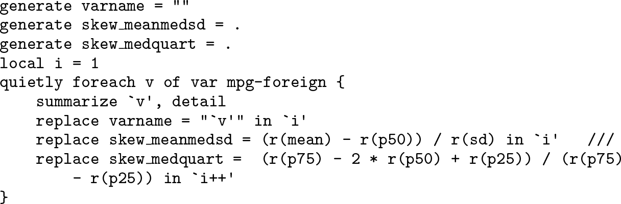
Some new details here deserve spelling out. We need to initialize each variable we are going to use. The recording of variable names here is rather more than an adornment. Because these values bear no relation to the structure of the existing dataset, the very first sort after this will destroy all links to the present order of the variables, so we should record variable names explicitly.

We are looping over variables, so in parallel we also need to loop over observations. Hence, we first initialize a local macro, here i to 1. After we put all the results for a particular variable in a particular observation, this can be incremented. For the names of particular r-class results, you will need to refer to the manual or (what is sometimes quicker) work them out by examining a return list. For e-class commands, the advice is similar but for ereturn list.

Once that is done, a graph can be produced, say,

scatter skew_*, mlabel(varname)

which, naturally, you may inspect for the auto data or, with different variable names, any interesting dataset. The auto data alone show one property of one measure that is unsurprising on reflection, but I will leave that as a hint, depending on whether you find the example interesting statistically, rather than just as an illustration of Stata technique.

This example should not be left before we grasp one awkward detail. Suppose that a variable were actually constant. In this situation, the standard deviation and interquartile range are both necessarily 0, and dividing by 0 makes any result indeterminate. In practice, this is likely to be unimportant, but in writing code it should become habit to think through what should happen if missing values arise.

The kind of approach described here may be compared with that in cookery programs. We all know that expert cooks sometimes make mistakes just like everybody else, except that they presumably do so less often than most others. What you see, however, lacks all the gaffes, small or large, which were edited out before publication. Similarly, this example was something I really wanted to do, but I did not get all the details right the first time. How you do it is up to you, but working your way up from the first beginnings to a more complete script in Stata’s Do-file Editor or another text editor is an approach that appeals to many Stata users.

All that said, another approach altogether is to set up saving results directly to a new dataset (see [P] postfile) or (in Stata 16 and up) to a new frame (see [D] frames). For a bundle of other tips in this territory, see Cox (2012b).

8 Conclusion

Each set of loops in parallel is just one loop, typically with forvalues or foreach, with actions in parallel. Devices that help include gettoken, macros as counters, the word # of syntax, and tokenize. In all of this, we need to know how local macros work and know about how Stata defines and uses words and tokens.

Interpreted suitably broadly, looping is much of programming if not most. Many themes could be added, including the use of [D] statsby, [D] collapse, and [D] contract.