2 Local macros
2.1 A character string given a special name
A macro in Stata is just a character string given a special name, so that you can then use that name, and Stata can understand that name, to refer to the contents of the character string. It is a way of setting up a mutually understood code.
If I type in Stata

then what I have done is assign the name rhsvars to the character string
"trunk weight length turn displacement"
That character string includes some variable names for the auto dataset bundled with Stata.
The quotes here, " ", delimit the string. In fact, " " often are not necessary, although I do recommend that you use them, at least until you know when you can omit them without ensuing difficulty. The " " do make clear exactly where the string starts and ends, but they are not part of the string themselves.
But what if you did want to include one or more " characters in a character string? We will examine this point later.
The name of the string is usually much shorter than the string to which it refers. Put differently, the most obvious reason for defining a macro is so that you can refer to it later, often repeatedly, and save yourself some typing. We can imagine these variables as appearing on the right-hand side of some model equations, hence our name rhsvars. We refer to it by using single quotes, `´, say,
. regress mpg `rhsvars´
Note carefully that the opening or left quote or backtick, `, differs from the closing or right quote or apostrophe, ´. On my keyboard, and on many others, the corresponding keys occur some distance apart: the ` key toward the top left, near Esc, and the ´ key toward the right of center, nearer Return. (Some Unix users may find that the backtick key has been mapped to something else. If so, using this stuff in Stata will be unnecessarily difficult until you find out how to undo that mapping.) Whatever your keyboard, using a pair of ´´ (or for that matter ``) will not work in Stata to indicate macro names. Here it is possible to be misled by several of the fonts that may be used within Stata: many represent closing quotes by a character more like ‘, which looks as if it might legitimately occur as one of a pair.
2.2 How Stata processes macro names: Substitution first
We need to understand a little of how Stata interprets a command line like that just given. Essentially, all macro names are substituted by their contents before Stata attempts to execute any command. This fact is crucial to avoiding, or to debugging, some of the more subtle mistakes in using these commands. It is so important that I am going to single it out as the substitution first rule.
Let us go through that more slowly. Whenever you type a Stata command, Stata has two main things to do. The first task is to receive your command and to translate it into its own private terms. The second task is to try to execute your command. What is crucial here is that the first task includes substitution (sometimes called expansion) of any macro names that you used in the command line. In the example just given, Stata sees the left quote symbol, `, a name, and the right quote symbol, ´, and thinks “Aha! a macro name!” It then looks to see whether that macro name has been defined. In this case, rhsvars has previously been defined as "trunk weight length turn displacement". Hence, Stata substitutes (expands) the macro name, so that it now sees the line
. regress mpg trunk weight length turn displacement
Trying to execute this command is then the second task that it has to do. Because we first read the auto data into memory, that should be straightforward.
But what could go wrong in handling a macro? The main pitfall is just getting the name slightly wrong. With local macro names, as with other names, Stata is case sensitive, so that upper- and lowercase letters are different: `RHSVARS´ and `rhsvars´ will mean different things, unless—exceptionally—you deliberately defined two macros with different names and the same contents. In addition, as is true almost everywhere else in Stata, Stata makes no attempt to correct your spelling.
1
Suppose that by mistake you typed the name of some macro that does not exist. For example, suppose you typed `rhsvar´ when you should have typed `rhsvars´ and you have not defined `rhsvar´. In general, Stata does not mind you doing this. It may complain about the consequences, which are indeed unlikely to be what you want, but referring to a nonexistent macro is not, in itself, an error. In fact, Stata programmers often do this, and properly used, it turns out to be a very useful feature. Moreover, as this example implies, Stata does not allow you to abbreviate macro names.
Stata’s attitudes on macro names may be a surprise to you. After all, Stata complains vigorously whenever it expects names of existing variables and you refer to a variable name that is not included in your data, a mistake that, once again, is most likely to be just a typo, as in typing summarize npg for summarize mpg. But it is the way Stata works. The rule is that a macro name that refers to nothing is substituted by nothing, that is, the empty string, "". So
. regress mpg `rhsvar´
would be seen by Stata as
. regress mpg
which happens to make perfect sense as a way of getting the mean of mpg and a t-based confidence interval but is unlikely to be what you wanted.
The local macros you have defined are not set in stone. They will fade away at the end of a session; exit Stata, and all your defined local macros vanish. Less existentially, you can redefine macros at will. Suppose you wanted to add the variable name gear_ratio to rhsvars. Here is one way to do it, just overwriting the old definition,
. local rhsvars "trunk weight length turn displacement gear_ratio"
and here is a better way of doing it, amending the old definition by adding to it:
. local rhsvars "`rhsvars´ gear_ratio"
How does that work? It is another example of the substitution first rule; all macro names are substituted by their contents before Stata attempts to execute any command. So Stata first substitutes `rhsvars´ by its definition. It now sees
. local rhsvars "trunk weight length turn displacement gear_ratio"
and it then executes the command that specifies, which happens to redefine the macro. This looks exactly the same as the first way of doing it, so why did I say that the second was better, because we obliged Stata to do the extra work? One reason is that Stata will be far faster than you are at substituting the contents for the name and less error prone. An even more compelling reason is that it is a natural and helpful way of writing any operation in which we accumulate results step by step.
What often happens somehow—and more will be explained later—is that we loop around a statement like
. local results "`results´`new´ "
where `new´ refers to some new result. If the macro results is undefined when Stata comes to this statement, that is not a problem. The local macro results would then be created with the value of local macro new, followed by a space. Note the detail of the space, usually needed to separate elements of the list of results. This is useful even for accumulating simple lists like 1 2 3 4 5, even though there are other ways of doing that, principally through numlist (see [P] numlist).
If the macro results is already defined when Stata comes to this statement, then whatever is in new will just be appended to the existing value of results. Either way, we are seeing a method of accumulating results one by one.
Macros can be redefined not only readily but also as empty—a key special case of redefining. To reverse a previous notion, a macro redefined as empty by
. local whatever
or by
. local whatever ""
ceases to exist.
2.3 What does “local” mean?
We have yet to explain the jargon local. As its geographical counterpart implies, macros are visible within some space, a name space: that is, local macros are visible only within the Stata program in which they are defined. An interactive session counts as a Stata program, as does any other program, whether one that is defined as such (given its inclusion between a program define or program statement and an end statement); or one that is so by courtesy (that is, a do-file or a set of commands in Stata’s Do-file Editor).
What does this mean? Suppose again that you have defined local macro rhsvars. What would happen if you run a Stata program written by StataCorp programmers, or by a Stata user, or—if you are a programmer yourself—by you on some previous occasion, and that program also uses some local macro rhsvars? This is more likely than you might think, even if you do not program yourself and you never use anything not in official Stata, because the majority of commands in official Stata are defined by Stata programs. But even if, by sheer coincidence, another program includes the same name, it is not a problem at all, because the two macros are totally distinct and never confused by Stata. And this is precisely what local means: visible only locally, within a program. While somebody else’s program is running, Stata sees and works with his or her rhsvars. Even if it is changed during the running of a program, that has no effect on your rhsvars. That principle is vital for using local macros because otherwise you would need to look inside every program you used and check for possible incompatibilities.
2.4 Global macros
There are, in contrast to local macros, macros in Stata that are visible everywhere, irrespective of what program is running, Stata itself (an interactive session), or a program so defined, or a do-file. These are called global and defined similarly:
. global rhsvars "trunk weight length turn displacement gear_ratio"
They are referred to in a slightly different way, for example,
. regress mpg $rhsvars
The single $ flags the start of a macro name. Occasionally, you may need to avoid possible confusion by using braces as well, as in ${rhsvars}. Although global macros have important uses, and quite possibly you may have used some already, I will say very little more about them in this column. What we are discussing needs only local macros, and even though global macros could be used for some of the same purposes, there is a risk that your global macros and somebody else’s global macros could get confused. Indeed, the whole point about global macros is that multiple definitions cannot coexist.
2.5 Macros can contain numeric characters
Although we have defined macros as character strings, those strings in Stata very often include numeric characters only. Hence, we frequently think of such macros as having numeric values. That piece of news may have been another surprise. You may be accustomed to the sharp division between string and numeric variables, as shown by the special methods you need to cross it, such as the encode, decode, destring, and tostring commands. In fact, this double aspect of macros is largely a useful illusion, one that turns out to be yet another example of the substitution first rule. In other words, macros really are just strings: it is just that the rest of Stata is happy to treat their contents as numeric whenever that makes sense.
For example, given the definitions
. local i 1
or
. local i "1"
Stata does the same thing: sets the local macro i to the character "1". As mentioned previously, the delimiters " " are usually optional. The character concerned happens to be a numeric character, but that causes no problem. Now suppose we want to redefine the macro by incrementing by 1. If we are thinking numerically, what is most natural to us, and perfectly acceptable to Stata, is to write this as an evaluation:
. local i = `i´ + 1
To be precise, the equals sign flags to Stata that the expression that follows should be evaluated and it should feed the result of that evaluation to what precedes it. This is a new syntax compared with any examples we have seen so far but a syntax that is very useful. Following the substitution first rule, what Stata sees is
. local i = 1 + 1
It then evaluates the expression 1 + 1 and redefines the macro i as the result of the expression, namely, the number 2, which it is happy to treat as the numeric character "2". (That is a little more of a leap than you might think: remember that computers do their calculations in binary, not decimal.) The evaluation has nothing to do with the macro: it is part of the rest of Stata. That rest of Stata from context takes you to want + to be, as usual, the numeric operation addition. But suppose the expression was
. local i = "1" + "1"
Here the quotes, " ", insist to Stata that the macros be treated as strings, for which purpose those quotes are essential. The rest of Stata from context takes you to want + to be the string operation concatenation, that is, adding the strings by juxtaposition. As a result, i will now contain the string "11". Again, they happen to be numeric characters, but "Stata " + "Corp" would have worked just as well.
Evaluations are also often used to produce the results of string expressions, as in
. local lcstring = lower("`string´")
If you want to know more about string functions like lower(), see [FN] String functions.
Note finally that
. local i "`i´ + 1"
is different again. Given i of "1", what ends up as the new local i is just the string "1 + 1". Without the equals sign, no evaluation will take place, just substitution of the macro name by its existing contents. The same result would be produced by
. local i = "`i´ + 1"
because, given the surrounding quotes, the + character is treated as just another character and not an operator. Here there would be evaluation, but it makes no difference to the contents of the macro.
2.6 Compound double quotes
We left one point hanging in the air, namely, how to get the " character into a macro. The answer is to use so-called compound double quotes, `" and "´, as delimiters. The first marks the start, and the second marks the end of a macro. What is more, they themselves can be nested within a macro definition as in

For more on this, see [U] 18.3.5 Double quotes.
4 foreach
4.1 A first example
One way to do it is with foreach, and it provides us with our first example:
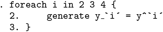
Now that we know that `i´ refers to a local macro name, the structure should seem less mysterious. More precisely, this is an example of one possible syntax with foreach, so we will back up and explain that more generally.
4.2 First syntax
Using more ordinary words, yet also a little abstraction,
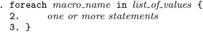
The structure concisely encapsulates several features:
A macro name must be given in the first part of the foreach structure.
A list must be specified immediately after. In the syntax given here, in list, the keyword in specifies that you are going to spell out all the individual elements of the list. (That wording is a bit strained, but I find it helps me to remember the syntax.) There is another syntax, which we will see in a moment.
One or more statements must be given within braces, { }. Usually, at least one of those statements refers to the macro name. Quite how you space them out between those braces is up to you so long as each statement occurs on a separate line. I like to indent commands by one tab, but that is a matter of personal taste. Stata does not care about indenting, but you should: poorly laid out code is more difficult to read, to understand, and to modify than well-laid-out code. (For one very helpful general statement on code style, see chapter 1 of Kernighan and Pike [1999].)
The foreach structure automatically defines the macro in turn as each of the members of the list and then substitutes its contents in any macro references in the commands within the braces. In our case, the result is the three commands given earlier.
The macro disappears at the end of the foreach structure. Thus, you will lose any preexisting macro with the same name. If you are in the habit of using many local macros interactively, you may want to devise your own conventions for names to be used only with structures such as foreach.
Let us look at another problem: producing transformations of several variables, supposing, say, that positive skewness is our main concern and that we are considering square root, logarithmic, and reciprocal transformations. Given three transformations and possibly many more variables than that, you should prefer to loop through a list of variables:

However, Stata allows several ways of giving abbreviated variable lists (varlists in Stata jargon), especially wildcards and variable ranges, as detailed at [U] 11.4.1 Lists of existing variables. Such features can be exploited with foreach by using the second syntax referred to just now.
4.3 Second syntax

The keyword of specifies that you are going to give a list of the type to be named. (That wording may also serve as a mnemonic.) In our last example, the listtype is varlist, so, if we had just been inspired by reading Tukey (1977) to try transforming everything numeric, we could try

The capture here is a device to catch the occasions when a command will not work. It has many uses in this territory. The notion is easy to grasp: if the following command does not work, then just digest the output (including the error) and carry on regardless. The alternative, without capture, is that foreach will stop at the first statement that does not work, leaving you very often with a partly completed task. See [P] capture for more examples.
Why might the generate commands not work? Suppose in our case that the variables in memory included some string variables, so that any attempt to take logarithms or square roots or reciprocals of those variables would fail. The solution is to say, by means of capture, “unless this will not work”.
Another reason they might not work is whenever you have variable names very near the current 32-character limit on length, such that the new name implied by log`x´ or sqrt`x´ causes an error message. In this case, and in others, we might want to carry on regardless, but still get an informative message, to see whether we need to sort out any problems afterward. There are several ways of doing this, but here is one, for simplicity shown with only the logarithmic transformation:

As the documentation for capture explains, Stata commands that fail produce a so-called return code that is not zero. capture puts the return code in _rc, so that it is accessible. The second line of code in this example displays the name of the offending variable and the return code whenever that is not zero, using the command if (see [P] if) and also the fact that if _rc is always equivalent to if _rc ˜= 0, as explained in a previous column (Cox 2002, sec. 5).
We have seen a listtype that is a varlist. foreach also allows four other types of list: those given within a local; a global; a newlist (that is, a list of new variable names; see [U] 11.4.2 Lists of new variables); or a numlist (that is, a list of numbers, see [U] 11.1.8 numlist or [P] numlist). So an earlier example could be written in terms of a numlist,

with no real gain in this case, beyond showing the principle. In passing, note that three-letter abbreviations like num are permissible for each listtype.
In general, this second syntax is much more powerful and more useful than the first: if your list contains tens, hundreds, or thousands of elements, you clearly do not want to be obliged to specify all of them, and the indirection made possible by (say) varlist or numlist notation is extremely helpful. What is more, Stata is often faster at cycling through lists given in this second syntax.
One very common application of foreach is just to produce univariate results for each of several variables. Sometimes, a Stata command producing univariate results permits a varlist containing several variable names, while sometimes, such a command may be used only with a single varname. foreach can be used as a wrapper to cycle through a varlist whenever only a single varname is acceptable. For example, let us imagine that we are drawing normal quantile plots (also known as normal probability plots or probit plots) using qnorm. See [R] Diagnostic plots if more information is needed. The syntax diagram of qnorm shows that it allows only the varname syntax, so we wrap a generic call inside a foreach:

set more on followed within the loop by more here ensures that each graph remains visible for as long as we wish to scrutinize it (see [P] more). As before, the capture device is available should it be needed. In this case, we would need capture noisily because capture alone would swallow the graph as well as any error message (see [P] quietly). Naturally, an alternative is just to make the effort to be sure that the varlist supplied contains only appropriate variables, in this example, only numeric variables that we wish to check for normality. After the loop, set more off reverts to Stata’s default (as from Stata 15).
4.4 Do not confuse the two syntaxes
The in and of syntaxes are distinct and should not be confused. In particular, it is legal in Stata to have a structure that begins something like
. foreach q in numlist 1/3 {
Any kind of list may follow in, so Stata will not pick up that this is almost certainly an attempt at
. foreach q of numlist 1/3 {
although you will learn from the consequences of the first that it was not what you wanted. Thus, any way of keeping the in and of syntaxes separate in your mind, such as the mnemonics suggested earlier, may be of help.
5 forvalues
forvalues is complementary to foreach. It can be thought of as an important special case of foreach for cycling through certain types of numlist but presented a little more directly.

Here the range_of_values specifies a sequence of numbers and takes one of two main forms, exemplified by 1/10 and 10(10)100. The first is shorthand for 1 2 3 4 5 6 7 8 9 10, that is, integers from 1 to 10. The second is shorthand for 10 20 30 40 50 60 70 80 90 100, that is, integers from 10 to 100 in steps of 10. Clearly, 1(1)10 would be another way of specifying the first example. For decreasing sequences, use a form like 25(-1)1.
There are yet more possible ways of specifying ranges. 10 20:100 and 10 20 to 100 are equivalents to 10(10)100, which you may use if you prefer.
In short, whenever you want to cycle over a simple sequence of integers, forvalues is an alternative to foreach. foreach must store the integers, whereas forvalues calculates them one by one, giving it an edge in speed of execution.
Using forvalues gives a possible alternative to our first example with foreach, generating powers of a variable:

For a new example, let us again imagine that we are drawing normal quantile plots using qnorm. One key issue in assessing the variability on such plots is how much variability would be expected even if the parent distribution really were exactly normal (Gaussian). Suppose our variable’s normal quantile plot is produced and named by a line such as
. qnorm ourvar, name(ourvar)
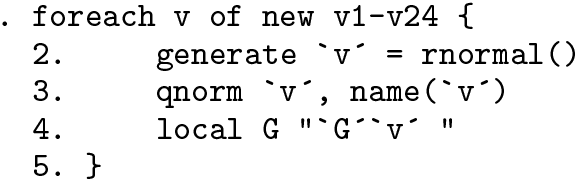
It is helpful to be able to compare such a plot with a reference portfolio of plots for normal samples of the same size. Such a procedure is suggested, for example, by Wild and Seber (2000) in their excellent text (p. 413). This qnorm command would use every value of ourvar (so long as no values were missing; we will set that possible complication on one side). Knowing Stata’s predilection for showing multiple graphs in a k × k array, we will go for 5 × 5 as a modest number of graphs that remain fairly legible individually. Given the existing plot already named ourvar, we need 24 random samples and their normal probability plots. As a matter of good practice, set seed first for reproducibility.
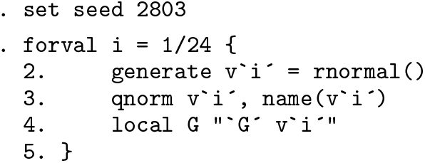
As the local macro i goes from 1 to 24, at each step, we get a new sample from a standard normal N(0, 1) by using the rnormal() function. We then use qnorm to draw a normal quantile plot, which will flash by, but we name each graph with the same name as the variable. We accumulate the names of the variables (and thus the .gph files) in a local macro G.
Now all the ingredients are ready. We can just combine our named graphs:
. graph combine ourvar `G´
To recap on the forval structure: the macro created, namely, i, runs over the values 1 through 24. It is substituted in turn as a part of a new variable name (for example, v`i´ becomes v1) and as part of a new graph name (same example, different context). We see also an illustration of an important principle: such a structure can be as valuable for its side effects—in this example, the named graphs left behind—as for its immediate and obvious effects. But most clearly of all, typing this is a large saving on repeating a generate command and a qnorm command for each of 24 variables. And the reference graphs remain of use if we want to look at other variables in this way.
This is not the only way to do it. You might prefer to use foreach,
which has at least one advantage: a side effect of declaring listtype to be newlist is that Stata would check before entering the loop that no existing variables had any of the variable names v1-v24.
6 Initializing before foreach or forvalues
In all the examples so far, we have been able to set up our foreach or forvalues loop straightaway. There are many problems, just a little more complicated, in which we need one step more, namely, to initialize one or more things before we enter the loop. This can arise in various ways, and we will look at two. We might want to create a new variable, but the recipe for creation is too complicated for a single command. (The limit is likely to be inherent not so much in Stata’s syntax as in our own need to keep things simple, but therein is no shame and much benefit.) Or we might want to populate a matrix with entries from separate calculations.
6.1 Initializing a variable
Such tasks often arise in cleaning up fairly large datasets containing string variables, say, names of countries or companies or diseases. If the dataset has been produced by, or from the responses of, several people, or even by one person, there may be various small inconsistencies. To be safe, we keep the original variable but work first at producing a more consistent version. If we are happy with our work, we might be bold and drop the original.
Imagine a survey with a question on vacation destinations. Respondents were asked to state countries they wished to visit. Initial inspection reveals, among many other details, a multitude of near synonyms for Britain: Britain, Great Britain, UK, United Kingdom, and so forth.
2
We decide to combine these all into Britain.
A constraint on this is that we can use generate only once: thereafter, we can make any number of changes, but they must be done through replace. It is often advisable therefore to put a generate statement outside the loop as in

Three extra details arise here. First, when we produce a copy of a string variable for cleaning, pushing it first through trim() and itrim() removes leading and trailing spaces and tidies up internal spaces. That often helps and rarely hinders.
Second, note how strings with embedded spaces such as "Great Britain" need delimiting quotes.
Third, the subinstr() function is explained at [fn] String functions.
6.2 Populating a matrix
Many statistical commands produce single-number statistics that we might want to display in the form of a table. Some commands do this already. For example, correlate does this automatically: given a varlist of numeric variables, it will produce a correlation matrix. However, other commands are not set up to do that. foreach makes it possible to overcome that in a relatively straightforward way. This example is a little more complicated than any so far. If you are trying to copy this in your own Stata or to modify it to fit a related problem of your own, you will probably want to make use of a text editor, which could be Stata’s own Do-file Editor or any other text editor you prefer.
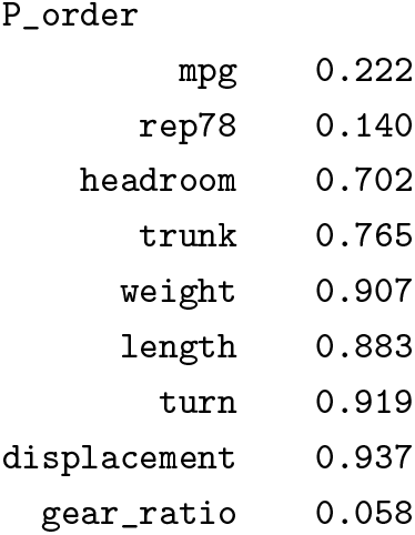
Consider ranksum, which takes a response variable and a grouping variable that defines precisely two groups and carries out a Wilcoxon–Mann–Whitney test. (See [R] ranksum.) The command has an interesting option porder, which calculates the probability
pr(variable in group 1 > variable in group 2)
that values in one group are higher than in the other group. Although this is not the place to argue the case in detail, my prejudice is that this descriptive measure (estimated parameter, if you wish) is often more useful than a p-value for the test. A little unusually, 0.5 is the reference level as defining the state in which values in group 1 being larger than those in group 2 occurs just as often as the other way round. Thus, probabilities being near 0 or near 1 are both of considerable interest.
Suppose we want to look systematically at results for the auto data. We will set aside the string variable make and use the binary variable foreign as grouping variable and then look at the other variables, price-gear_ratio, all regarded as response variables. The check is thus whether foreign cars are systematically different from domestic cars, those made in the United States.
In computing as in cookery, it is customary to show only successful recipes, but be assured: it is not trivial to get to code like this without a series of corrections and improvements.
We need a foreach loop over variables. But this problem is also typical of many others in needing actions both before and after the loop. In particular, we use a small trick to ensure that precisely the same observations are used in each ranksum command. If we run a regression with all the variables, only the observations with nonmissing values on all variables will be included. Hence, we can use e(sample) as an indicator function copied to an indicator variable:

Follow Stata as it goes through the structure. It extracts price as the first variable of the varlist price-gear_ratio and sets that as the first instance of local macro v. Then, Stata substitutes the macro names by their contents and executes ranksum price if touse, by(foreign) porder.
Now what we need to do is pick up the result left behind in memory after ranksum is executed. The manual entry on each command, in a Saved Results section, will document any results that are temporarily accessible in Stata’s memory after a command is executed. “Temporarily” means until you exit Stata or until the next command of similar type is executed, whichever happens sooner. If the manual entry is not accessible, typing either return list or ereturn list immediately after a command will show what is saved where. The rule of thumb is to try return list first unless the command can be thought of as estimating a model, in which case try ereturn list first. In our case, using either the manual or return list, we find that we need to pick up r(porder). Then, results are added as a new row in the matrix results. nullmat() catches the first time around the loop when that matrix does not exist.
At this point, Stata has completed one step through the loop. It continues cycling through the varlist until the last variable, executing ranksum as detailed for gear_ratio.
Let us underline the careful treatment here of missing values. Left to its own devices, Stata will use as many observations as possible. With the auto data, this will be 74, unless one of the variables is rep78, for which 5 values are missing, so that it will be 69. This behavior may be what you want, but it seems more likely that you would prefer that the same observations are used in every calculation.
Once we have finished the loop, it is a matter of adding detail to the matrix and then listing it with a suitable format. Intelligible labeling of the rows and columns of the results matrix is very much worthwhile because it makes the result so much easier to read. Another command usually billed as a programming command, unab (see [P] unab), saves your typing. It “unabbreviates” (ugly word, but useful action) a variable list into a local macro, after which you can attach the names to the results matrix (see [P] matrix rownames). One column name here can be added similarly. In this case, three decimal places seem fine for the estimated probabilities, but naturally your problem may differ.
We are still some way from anything publishable or even very presentable, but we will not push the example further. We got this far.