Implementing quantile selection models in Stata

Abstract

In this article, we describe qregsel, a community-contributed command that implements a copula-based sample-selection correction for quantile regression recently proposed by Arellano and Bonhomme (2017, Econometrica 85: 1–28). The command allows the user to model selection in quantile regressions by using either a Gaussian or a one-dimensional Frank copula. We illustrate the use of qregsel with two examples. First, we apply the method to the fictional dataset used in the Stata Base Reference Manual for the heckman command. Second, we replicate part of the empirical application of the original article using data for the United Kingdom that cover the period 1978–2000 to compare wages of males and females at different quantiles.

1 Introduction

Nonrandom sample selection is a well-known issue in empirical economics. Since the seminal work of Heckman (1979) addressing this problem, much progress has been made in methods that extend the original model or relax some of its assumptions. For example, Vella (1998) provides a survey of methods for fitting models with sample-selection bias in this line.

Although most of the effort has been focused on models that estimate the conditional mean, the literature in econometrics has also tackled the problem of nonrandom sample selection in the context of quantile regression. For example, Arellano and Bonhomme (2018) offer a survey of recently proposed methods with a focus on a copula-based sample-selection model suggested in Arellano and Bonhomme (2017).

As discussed in Arellano and Bonhomme (2018), the flexible copula-based approach has an advantage over methodologies that are based on the control function approach. The latter impose conditions on the data that may not be compatible with quantile models if the model is nonadditive with nonlinear quantile curves on the selected sample (see Huber and Melly [2015]).

In this article, we briefly discuss the copula-based approach proposed by Arellano and Bonhomme (2017) and present a new community-contributed command called qregsel that implements it. ¹ In addition, we illustrate the method with two empirical examples. First, we fit a quantile regression model with sample selection using the Stata Base

Reference Manual example for the heckman command. Second, we replicate the analysis of wage inequality in the United Kingdom for the period 1978–2000 as in the original article.

This article is organized as follows. Section 2 describes the methodology. Section 3 describes the qregsel command and its syntax. In section 4, we illustrate the use of the command with the empirical examples, and we conclude in section 5.

2 Methodology

In this section, we briefly review the quantile selection model of Arellano and Bonhomme (2017). The goal is to obtain a consistent estimator when there is sample selection in a nonadditive model such as quantile regression, which precludes the use of the control function approach. The assumption of additive separability of observables and unobservables in the output equation does not hold in general, as argued by Huber and Melly (2015) in the context of testing.

2.1 The model

Sample selection is modeled using a bivariate cumulative distribution function (c.d.f.) or copula of the percentile error in the latent outcome equation and the error in the sampleselection equation. The copula parameters are estimated by minimizing a method-of-moments criterion that exploits variation in excluded regressors to achieve credible identification. Then the quantile regression parameters are obtained by minimizing a rotated check function, which preserves the linear programming structure of the standard linear quantile regression (see Koenker and Bassett [1978]).

Consider a general outcome equation specification where the quantile functions are

linear:

$Y^{\ast }=Q(U,\mathbf{\text{X}}) =\mathbf{\text{x}}\prime \beta (\tau )$

Y ^∗ is the latent outcome variable (for example, wage offers), the function Q is the τth conditional quantile of Y ^∗ given the covariates X (for example, education and experience), and U is the error term of the outcome equation. The participation equation is defined as

$D=\mathbb{I}\{V\le p(\mathbf{Z})\}$

where D takes values equal to 1 when the latent variable is observable (for example, employment) and equal to 0 otherwise, Z contains X and at least one covariate B that do not appear in the outcome equation (for example, a determinant of employment that does not affect wages directly), p(Z) is a propensity score, and V is an error term of the selection equation. Hence, we observe (Y, D, Z) where Y = Y ^∗ only when D = 1.

Under the set of assumptions ² detailed in Arellano and Bonhomme (2017), we have that the c.d.f. of Y ^∗ , conditional on participation and for all τ ∊ (0, 1), is

$\text{Pr}\{Y\ast \le \mathbf{\text{x}}\prime \beta (\tau )|D= 1,\mathbf{\text{Z}}=\mathbf{\text{z}}\}=Pr\{U\le \tau |V\le p(\mathbf{\text{z}}),\mathbf{\text{Z}}=\mathbf{\text{z}}\}=G_x\{\tau , p(\mathbf{\text{z}})\}$

where G_x ≡ C(τ, p)/p is the conditional copula function, which measures the dependence between U and V . Here G_x maps rank τ in the distribution of latent outcomes (given X = x) to ranks G_x {τ, p(z)} in the distribution of observed outcomes conditional on participation (given Z = z). Namely, the conditional G_x {τ, p(z)} quantile of observed outcomes (that is, when D = 1) coincides with the conditional τ quantile of latent outcomes, which implies that if we are able to estimate the mapping G_x (τ, p) from latent to observed ranks, we are able to recover Q(τ, x) from the observed outcomes (that is, we are able to estimate the τ quantile correcting for selection).

To implement the method, we assume that the copula function is indexed by a single parameter such that

$G_x(\tau ,p)\equiv G(\tau ,p;\rho )=\frac{C(\tau ,p;\rho )}{p}$

where the numerator is the unconditional copula of (U, V ), the denominator is the propensity score, and ρ is the copula parameter that governs the dependence between the error in the outcome equation and the error in the participation decision.

2.2 Estimation

Arellano and Bonhomme’s (2017) estimation algorithm can be summarized in three steps: estimation of the propensity score; estimation of the degree of selection via the c.d.f. of the percentile error in the outcome equation and the error in the participation decision; and then, using the estimated parameter, the computation of quantile estimates through rotated quantile regression.

The first step consists of estimating the propensity score γ by a probit regression:

$\widehat{\gamma }={\mathrm{argmax}}_a{\displaystyle \sum _{i=1}^N{D}_i}\ln \Phi \left(Z_i^{\prime }a\right)+\left(1-D_i\right)\ln \Phi \left(-Z_i^{\prime }a\right)$

The second step is to estimate ρ by minimizing a method-of-moments objective function, which allows us to obtain an observation-specific measure of dependence between the rank error in the equation of interest and the rank error in the selection equation. This is accomplished with a grid search over different values of ρ such that

$\widehat{\rho }={\mathrm{argmin}}_c‖{\displaystyle \sum _{i=1}^N{\displaystyle \sum _{l=1}^L{D}_i}}\phi \left({\tau }_l,Z_i\right)\left[1\left\{Y_i\le X_i^{\prime }\widehat{\beta }\left({\tau }_l,c\right)\right\}-G\left\{{\tau }_l,\Phi \left(Z_i^{\prime }\widehat{\gamma }\right);c\right\}\right]‖$

where ‖ · ‖ is the Euclidean norm, τ ₁ < τ ₂ < · · · < τ_L is a finite grid on (0, 1), and the instrument functions are defined as φ(τ, Z _i ), where the dim φ ≤ dim ρ, and

$\begin{array}{l}{\widehat{\beta }}_{\tau }(c)={\mathrm{argmin}}_{b(\tau )}{\displaystyle \sum _{i=1}^N{D}_i}\left(G\left\{\tau ,\Phi \left(Z_i^{\prime }\widehat{\gamma }\right);c\right\}{\left\{Y_i-X_i^{\prime }b(\tau )\right\}}^{+}\right.\\ \left.\hspace{0.17em}+\left[1-G\left\{\tau ,\Phi \left(Z_i^{\prime }\widehat{\gamma }\right);c\right\}\right]{\left\{Y_i-X_i^{\prime }b(\tau )\right\}}^{-}\right)\end{array}$

where a ⁺ = max{a, 0}, a⁻ = max{−a, 0}, and the grid of τ values on the unit interval as well as the instrument function are chosen by the researcher. ³

Finally, using $\widehat{\gamma }$ and $\widehat{\rho }$ obtained above, the third step consists of computing ${\widehat{G}}_{\tau i}=G\left\{\tau ,\Phi \left(Z_i^{\prime }\widehat{\gamma }\right);\widehat{\rho }\right\}$ for all i to estimate β(τ) by minimizing a rotated check function of the form

$\widehat{\beta }(\tau )={\mathrm{argmin}}_{b(\tau )}{\displaystyle \sum _{i=1}^N{D}_i}\left[{\widehat{G}}_{\tau i}{\left\{Y_i-X_i^{\prime }b(\tau )\right\}}^{+}+\left(1-{\widehat{G}}_{\tau i}\right){\left\{Y_i-X_i^{\prime }b(\tau )\right\}}^{-}\right](1)$

where $\widehat{\beta }(\tau )$ will be a consistent estimator of the τth quantile regression coefficient.

Note that the third step is unnecessary if the quantiles of interest are included in the set τ ₁ < τ ₂ < · · · < τ_L used in the second step.

2.3 Copulas

The Arellano and Bonhomme (2018) analysis covers the case where the copula is left unrestricted, but for the implementation they focus on the case of identification where the copula depends on a low-dimensional vector of parameters.

In our empirical implementation, we consider only the case of a reduced set of onedimensional copulas. We include the Gaussian and a one-parameter Frank. Table 1 provides their respective functional forms.

Table 1.

Copula functions.

Copula name	C(U, V ; ρ)	Range of ρ
Gaussian	Φ2{Φ − 1(U), Φ − 1(V ); ρ}	−1 ≤ ρ ≤ 1
Frank	$-{\rho }^{-1}\log \left\{1+\frac{\left(e^{-\rho U}-1\right)\left(e^{-\rho V}-1\right)}{\left(e^{-\rho }-1\right)}\right\}$	−∞ ≤ ρ ≤ ∞

2.4 Measures of dependence

The parameter ρ, which governs the degree of dependence, is not directly comparable across copulas (see Hasebe [2013]). For this reason, researchers often report Kendall’s τ or the Spearman rank correlation coefficient as a measure of the degree of dependence. Both measures take the range of [−1, 1], where a value closer to 1 (−1) indicates a stronger (negative) dependence, and (in the case of our copulas) can be expressed as closed form in terms of ρ (see table 2).

Table 2.

Copula functions and measures of dependence.

Copula name	Range of ρ	Kendall’s τ	Spearman’s rank correlation
Gaussian	−1 ≤ ρ ≤ 1	$\frac{2}{\pi }{\sin }^{-1}(\rho )$	$\frac{6}{\pi }{\sin }^{-1}(\rho /2)$
Frank	−∞ ≤ ρ ≤ ∞	$1+\frac{4}{\rho }\left\{D_1(\rho )-1\right\}$	$1+\frac{12}{\rho }\left\{D_2(\rho )-D_1(\rho )\right\}$

NOTE: D_n (ρ) is a Debye function, where $D_n(\rho )=\left(n/{\rho }^n\right){\displaystyle {\int }_0^{\rho }\left\{\left(t^n\right)/\left(e^t-1\right)\right\}}dt$ .

2.5 Rotated quantile regression

As previously mentioned, the quantile estimates are obtained by minimizing a rotated check function [see (1)]. The minimization problem can be written as the linear programming problem ⁴

${\mathrm{Min}}_{{\beta }_{\tau },u,v}{\displaystyle \sum _{i=1}^N{\widehat{G}}_{\tau i}}{u}_i+\left(1-{\widehat{G}}_{\tau i}\right)v_i$

such that

$\begin{array}{l}\mathbf{\text{y}}-\mathbf{\text{X}}{\beta }_{\tau }=\mathbf{\text{u}}-\mathbf{\text{v}}\hfill \\ \mathbf{\text{u}}\ge {\mathbf{\text{0}}}_n\hfill \\ \mathbf{\text{v}}\ge {\mathbf{\text{0}}}_n\hfill \end{array}$

where 0 _n is a vector of 0s, X is the matrix of observations of the covariates, y is the vector of observations of the outcome, and u and v are added to the inequality constraint to transform it into an equality.

This linear programming problem could be solved using the LinearProgram() class in Stata or, alternatively, using the Stata integration with Python. However, we implement an interior point algorithm developed by Portnoy and Koenker (1997) by translating the MATLAB code used by Arellano and Bonhomme (2017) to Mata language. ⁵

3 The qregsel command

In this section, we describe the qregsel command, which implements a copula-based sample-selection correction in quantile regression.

3.1 Syntax

The syntax of the qregsel command is qregsel depvar indepvars [if] [in] , select( [depvar _S =] varlist _S ) quantile(# [# [# …]] ) [copula( copula ) noconstant finergrid coarsergrid rescale nodots]

3.2 Options

select( [depvar_S =] varlist_S ) specifies the selection equation. If depvar_S is specified, it should be coded as 0 and 1, with 0 indicating an outcome not observed for an observation and 1 indicating an outcome observed for an observation. select() is required.

quantile( # [# [# …]] ) specifies the quantiles to be estimated and should contain

numbers between 0 and 1, exclusive. Numbers larger than 1 are interpreted as percentages. quantile() is required.

copula( copula ) specifies a copula function governing the dependence between the errors in the outcome equation and the selection equation. copula may be gaussian or frank. The default is copula(gaussian).

noconstant suppresses the constant term in the outcome equation.

finergrid finds the value of the copula parameter by using a grid of 199 values (values such that the Spearman rank correlation is approximately [−0.99, −0.985, …, 0.985, 0.99]) instead of 100 (values such that the Spearman rank correlation is approximately [−0.99, −0.98, …, 0.98, 0.99]), as done by default.

coarsergrid finds the value of the copula parameter by using a grid of 50 values (values such that the Spearman rank correlation is approximately [−0.99, −0.95, …, 0.93, 0.97]) instead of 100 (values such that the Spearman rank correlation is approximately [−0.99, −0.98, …, 0.98, 0.99]), as done by default.

rescale transforms the independent variables in the outcome equation by subtracting from each its sample mean and dividing each by its standard deviation.

nodots suppresses progress dots that indicate status over the grid search.

3.3 Stored results

qregsel stores the following in e():

3.4 Prediction

After the execution of qregsel, the predict command is available to compute a counterfactual of the outcome variable corrected for sample selection. The syntax is

predict newvarlist [if] [in]

where newvarlist must contain the names for two new variables: the first one for the counterfactual outcome variable and the second one for a binary indicator of selection.

The counterfactual outcomes are constructed by randomly generating an integer q between 1 and 99 for each individual in the full sample and then using the quantile coefficients associated with each draw of q to produce a prediction of the qth quantile of the outcome distribution. This approach follows the conditional quantile decomposition method of Machado and Mata (2005) and has been recently applied, for example, in Bollinger et al. (2019).

The selection indicator is generated by randomly drawing values of the error in the selection equation V from the conditional distribution of V given U = u, derived from the chosen copula using the estimated copula parameter and the values of U randomly generated to create the counterfactual outcome variable in the previous paragraph. This approach follows the empirical exercise performed in Arellano and Bonhomme (2017).

3.5 Inference

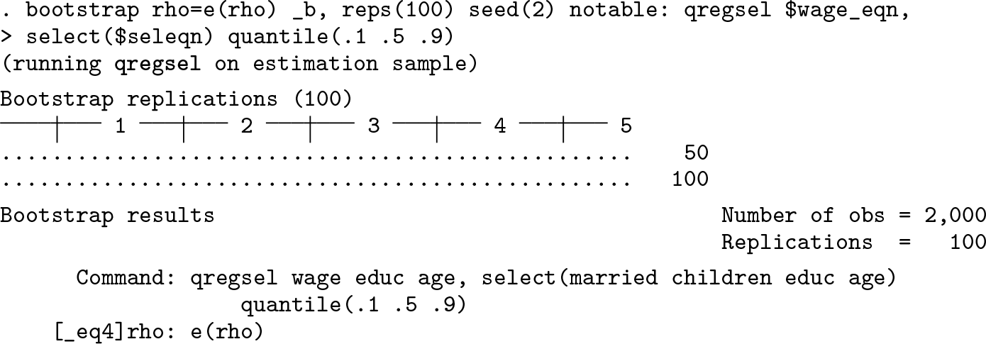
Confidence intervals for any of the parameters can be estimated using methods such as the conventional nonparametric bootstrap or, alternatively, using subsampling (see Politis, Romano, and Wolf [1999]) as done in Arellano and Bonhomme (2017) because of the computational advantage when using large sample sizes.

In our first empirical application, we illustrate how to use bootstrap to create a confidence interval for the estimated coefficients of the quantile regression and the copula parameter.

4 Empirical examples

In this section, we illustrate the use of the command with two empirical examples. First, we use the classic example of wages of women, in which we use the data available from the Stata manual example for the command heckman. Second, we replicate part of an exercise presented in Arellano and Bonhomme (2017) with data from the United Kingdom.

4.1 Wages of women

In this application, we use the fictional dataset used in the documentation of the Heckman selection model in the Stata Base Reference Manual (see StataCorp [2021a]) to study wages of women. As in the example, we assume that the hourly wage is a function of education and age, whereas the likelihood of working (and hence the wage being observed) is a function of marital status, the number of children at home, and (implicitly) the wage (via the inclusion of age and education). We do not take the logarithm of wage as it is usually done; however, the variable in the fictional dataset already has a bell-shaped histogram. In addition, we follow the example in the Stata 17 Base Reference Manual by not including squared age because it is standard in this type of regression.

First, we estimate a quantile regression over the quantiles 0.1, 0.5, and 0.9 without corrections for sample selection as a benchmark.

Next, we turn to the estimation of a quantile regression accounting for sample selection by using the command qregsel with a Gaussian copula. In addition, we plot the value of the objective function over the minimization grid (see figure 1). The value of ρ that minimizes the criterion function is approximately equal to −0.65, as stored in e(rho). The interpretation of this estimated value is that women with higher wages (higher U) tend to participate more (lower V ).

Figure 1.

Grid for minimization

After the estimation, a counterfactual distribution that is corrected for sample selection may be generated with the postestimation command predict as follows. Figure 2 displays the ventiles of the distribution corrected for sample selection versus the uncorrected one. We can see how wages are lower after correcting for selection at each ventile of the distribution.

Figure 2.

Corrected versus uncorrected quantiles

Finally, we illustrate the use of the bootstrap command to construct a confidence interval for the coefficients associated to three different quantiles and the copula parameter ρ using 100 replications.

4.2 Wage inequality in the United Kingdom

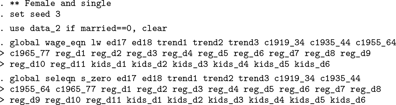
In this example, we apply the model to measure market-level changes in wage inequality in the United Kingdom. We compare wages of males and females at different quantiles of the wage distribution, correcting for selection into work. We replicate Arellano and Bonhomme (2017) using the dataset provided by the authors, which originally comes from the Family Expenditure Survey from 1978 to 2000. ⁶

We model log-hourly wages Y and employment status D. The controls X include linear, quadratic, and cubic time trends, 4 cohort dummies (born in 1919–1934, 1935–1944, 1955–1964, and 1965–1977, omitting 1945–1954), 2 education dummies (end of schooling at 17 or 18 and end of schooling after 18), 11 regional dummies, marital status, and the number of kids split by age categories (6 dummies, from 1 year old to 17–18 years old).

The excluded regressor follows Blundell, Reed, and Stoker (2003) and corresponds to their measure of potential out-of-work (welfare) income interacted with marital status. This variable was constructed for each individual in the sample by using the Institute of Fiscal Studies tax and welfare-benefit simulation model.

Arellano and Bonhomme (2017) fit the sample-selection model independently by gender and marital status. We replicate (see code below) the exercise reported in the article using a Frank copula and find that the copula parameter in the case of married individuals is −1.548 for males and −1.035 for females (the associated rank correlations are −0.250 and −0.170, respectively). For single individuals, the copula parameter is −7.638 for males and −0.421 for females (the respective rank correlations are −0.790 and −0.070). After the estimation using each subsample, we use predict to generate counterfactual outcomes, which are then used to plot quantiles by gender with and without correction for sample selection over time. We are able to replicate the empirical facts documented in the original article (see figure 3). We see that correcting for sample selection makes an important difference at the bottom of the wage distribution for males, while the difference seems to be less important for females.

Figure 3.

Wage quantiles by gender. notes: Quantiles of log-hourly wages, conditional on employment (solid lines) and corrected for selection (dashed). Male wages are plotted in thick lines, while female wages are in thin lines.

5 Concluding remarks

In this article, we introduced a new community-contributed command called qregsel, which implements a copula-based method proposed in Arellano and Bonhomme (2017) to correct for sample selection in quantile regressions. The use of the command was illustrated with two empirical examples.

Additional empirical applications of the econometric method here implemented included the analysis of the gender gap between earnings distributions in Maasoumi and Wang (2019) and the analysis of earnings inequality correcting for nonresponse in Bollinger et al. (2019).

7 Programs and supplemental materials

Supplemental Material, sj-zip-1-stj-10.1177_1536867X211063148 - Implementing quantile selection models in Stata

Supplemental Material, sj-zip-1-stj-10.1177_1536867X211063148 for Implementing quantile selection models in Stata by Ercio Muñoz and Mariel Siravegna in The Stata Journal