
Abstract
In this article, we present the
1 Introduction
In this article, we present the command
Unlike prior methods, the method implemented in
The remainder of the article is organized as follows. In section 2, we recall the setup of the semiparametric endogenous sample-selection model considered in D’Haultfœuille, Maurel, and Zhang (2018) and describe the data-driven procedure used to choose the quantile index for the extremal quantile regression. In section 3, we describe how to implement the method in practice. In section 4, we present the
2 The framework and estimation method
2.1 Model and estimation
We consider the outcome equation
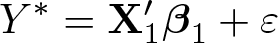
where Y
∗ ∊

where

The effect of
Y
∗ is not directly observed. Instead, and denoting by D the selection dummy, the econometrician observes only D, Y = DY
∗, and

In some cases, it may be more plausible to impose that, conditional on having “small” outcomes (Y
∗ → −∞), selection is independent of the covariates. This case can be handled simply by replacing Y with −Y and
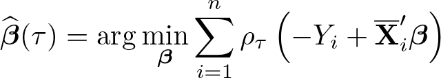
Combining (2) and (3), D’Haultfœuille, Maurel, and Zhang (2018, theorem 2.1) show that, under some regularity conditions on the upper tail of ε, as τ → 0,

Therefore, (4) suggests that we can estimate
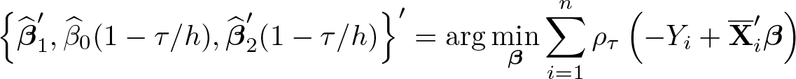
where
As is standard with extremal quantile regressions (see Chernozhukov, Fernández-Val, and Kaji [2018]), the rate of convergence is not the usual parametric root-n rate. Moreover, in this case, this rate depends on unknown features of the distribution of (D, Y
∗,
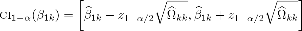
The results above rely on two main conditions, namely, (2) and (3). Importantly, we can develop a specification test of these conditions based on the implication that the coefficients

where
2.2 Choice of the quantile index
The performance of extremal quantile estimators depends on a tradeoff between bias and variance, which is governed by the quantile index τn
used in the extremal quantile regression. In the following, we present the algorithm outlined in D’Haultfœuille, Maurel, and Zhang (2018), which selects a suitable quantile index based on estimators of the bias and the variance of
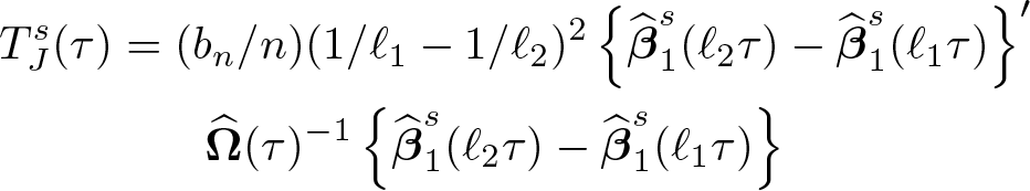
Specifically, consider the same test statistic as in (5), but where (ℓτn, τn ) are replaced by (ℓ 1 τn, ℓ 2 τn ), with ℓ 1 < 1 < ℓ 2:

D’Haultfœuille, Maurel, and Zhang (2018) show that the difference between the median of TJ (τ) and the median of a chi-squared distribution with d 1 degrees of freedom can serve as a proxy for the bias of the estimator.
The idea, then, is to estimate this difference using subsampling. 5 For each subsample and each quantile index τ within a grid G, one can compute TJ (τ). Let M sub(τ) denote the median of these test statistics over different subsamples for a given τ, and let Md 1 denote the median of the chi-squared distribution with d 1 degrees of freedom. Then, the proxy of the bias is defined as
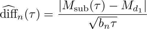
where bn denotes the subsample size.
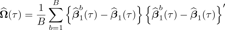
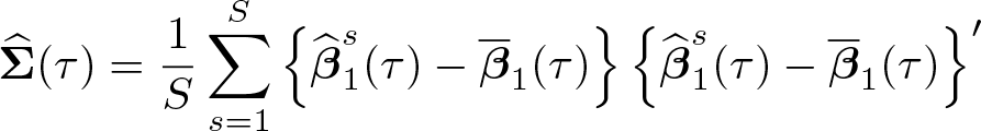
Similarly, the asymptotic covariance matrix is estimated by the covariance matrix of the subsampling estimator of
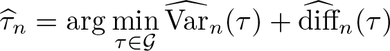
where G denotes a finite grid within (0, 1). This procedure results in undersmoothing compared with a more standard tradeoff between variance and squared bias. As with the case of nonparametric regressions, this is needed to control the asymptotic bias that would otherwise affect the limiting distribution of the estimator. We refer to D’Haultfœuille, Maurel, and Zhang (2018) for simulation-based evidence that this choice leads to estimators that are both accurate and only very mildly biased, thus leading to reliable inference on
3 Implementation
We summarize how we implement the method described above in 1. Draw B bootstrap samples and B subsamples of size bn
. 2. For each τ ∊ G: a. Compute the estimator of
Let b. Compute
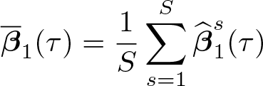
with c. Compute, for each subsample s = 1 …S, the estimator of
d. Compute e. Compute
with
3. Compute 4. Define
where 5. Compute
In practice, we consider an equally spaced grid G with lower bound min(0.1, 80/bn
), upper bound 0.3, and a number of points equal to nG
. The lower bound is motivated by the fact that if the effective subsampling size τbn
becomes too small, then the intermediate order asymptotic theory is likely to be a poor approximation (see Chernozhukov and Fernández-Val [2011] for a related discussion). To compute
4 The eqregsel command
We describe below the syntax, options, and stored results associated with the
4.1 Syntax
The syntax of
4.2 Description
X1 is the list of variables entering in
X2 is the list of variables entering in
4.3 Options

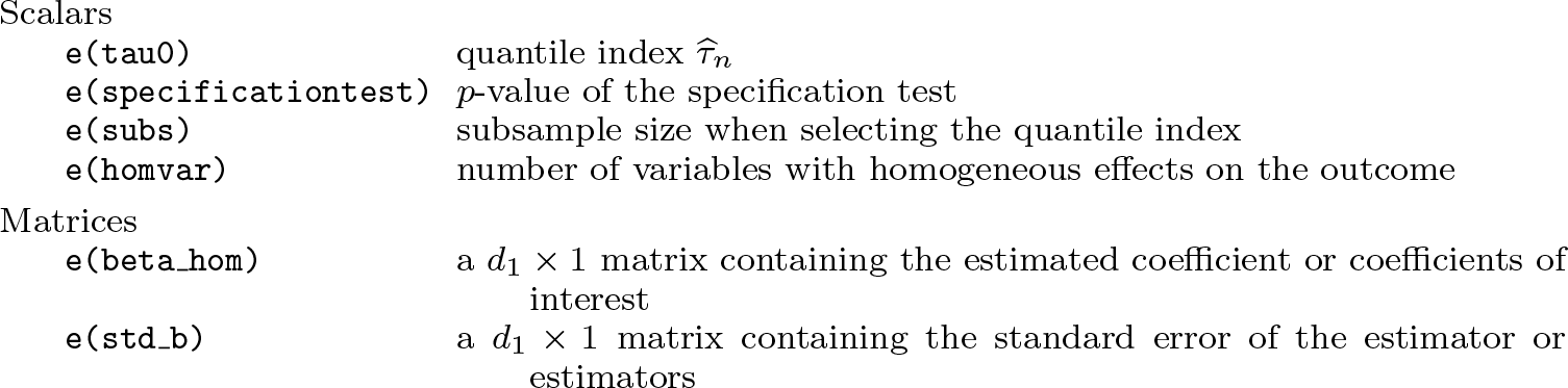
4.4 Stored results
5 Example
We use the command
We use the same samples and definitions of variables as D’Haultfœuille, Maurel, and Zhang (2018). In particular, we consider that an individual in the NLSY79 is a nonparticipant if he did not work in 1990 or in 1991. The outcome of interest is the (potential) log-wage, which is defined as the log of the mean real wages in 1990 and 1991 for workers who worked both years and the log of the real wage in the year of employment for those who worked only one year. We apply the same rules with the years 2007 and 2008 for individuals in the NLSY97.
In our specification, we estimate for the two samples the effect of the black dummy on the log of wages (
We report below the output of the
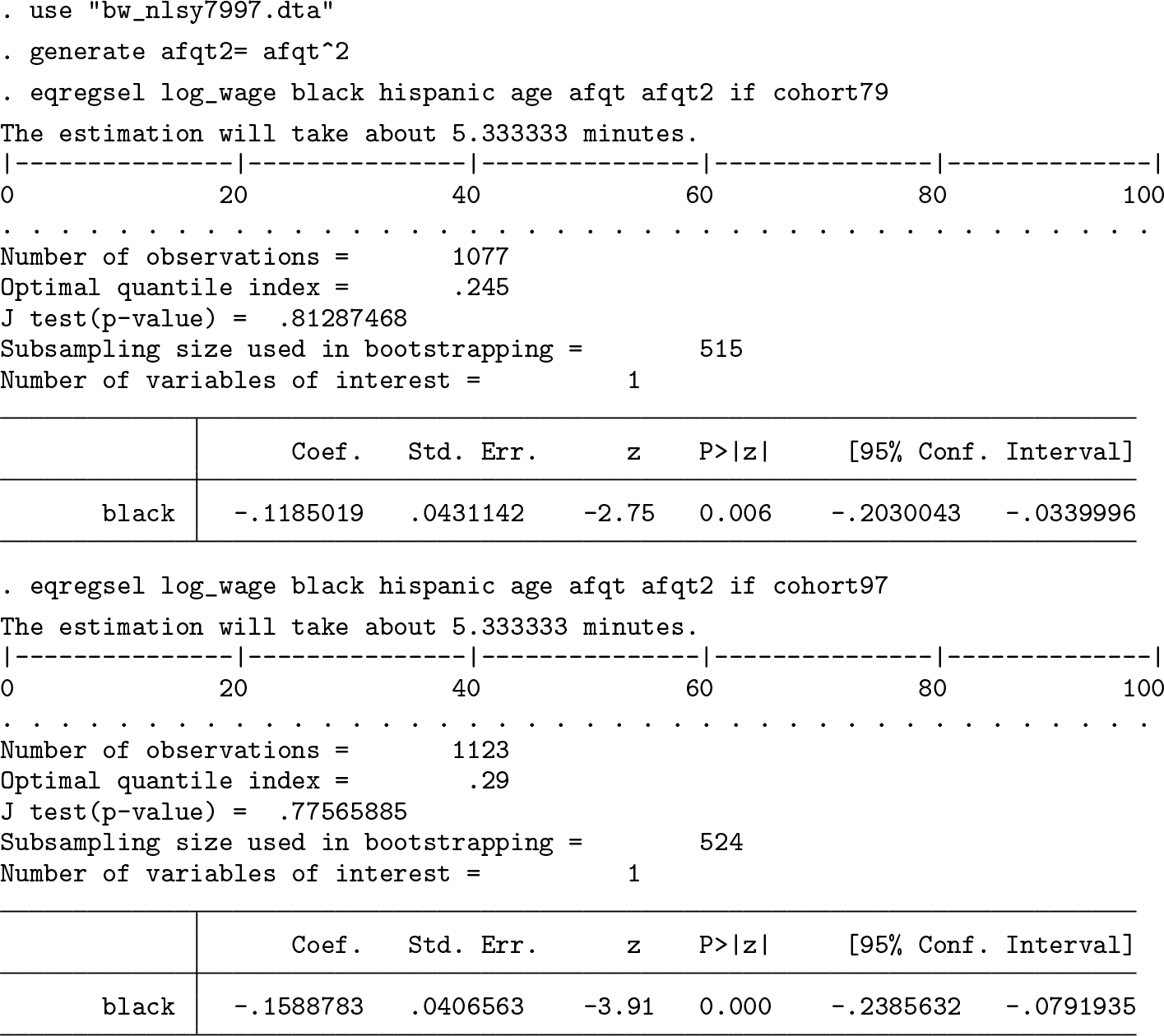
The estimation results point to statistically and economically significant black–white wage gaps for the two cohorts. We also observe a wider black–white wage gap for the 1997 cohort relative to the 1979 cohort, with an increase in the estimated gap from about 11.9% to 15.9%. Note, however, that the difference is not significant at usual levels (p-value = 0.51). Interestingly, the p-values of the specification tests imply that one cannot reject our specification for either cohort at any standard statistical level.
It is interesting to compare the estimated black–white wage gap with the results of a simple ordinary least-squares regression of the log of hourly wages on a black dummy and the same set of controls. The estimated black–white wage gap drops from 11.9% and 15.9%, for our specifications, to 8.1% and 9.7% (with standard errors equal to 0.035 and 0.041), for the ordinary least-squares specification that ignores selection. That the estimated wage gap is larger in magnitude when we use our method is consistent with the underlying sample-selection issue. Indeed, among males, blacks are significantly more likely to drop out from the labor market (Juhn 2003). Because dropouts tend to have lower potential wages, one can expect that not controlling for endogenous labor market participation will result in underestimating the black–white wage differential. 8
6 Conclusion
In this article, we have discussed how to use the
8 Programs and supplemental materials
Supplemental Material, st0598 - Estimating selection models without an instrument with Stata
Supplemental Material, st0598 for Estimating selection models without an instrument with Stata by Xavier D’Haultfœuille, Arnaud Maurel, Xiaoyun Qiu and Yichong Zhang in The Stata Journal
Footnotes
7 Acknowledgments
Yichong Zhang acknowledges the financial support from the Singapore Ministry of Education Tier 2 grant under grant no. MOE2018-T2-2-169 and the Lee Kong Chian fellowship.
8 Programs and supplemental materials
To install a snapshot of the corresponding software files as they existed at the time of publication of this article, type
Notes
References
Supplementary Material
Please find the following supplemental material available below.
For Open Access articles published under a Creative Commons License, all supplemental material carries the same license as the article it is associated with.
For non-Open Access articles published, all supplemental material carries a non-exclusive license, and permission requests for re-use of supplemental material or any part of supplemental material shall be sent directly to the copyright owner as specified in the copyright notice associated with the article.