Relative distribution analysis in Stata

Abstract

In this article, I discuss the method of relative distribution analysis and present Stata software implementing various elements of the methodology. The relative distribution is the distribution of the relative ranks that the outcomes from one distribution take on in another distribution. The methodology can be used, for example, to compare the distribution of wages between men and women. The presented software, reldist, estimates the relative cumulative distribution and the relative density, as well as the relative polarization, divergence, and other summary measures of the relative ranks. It also provides functionality such as location and shape decompositions or covariate balancing. Statistical inference is implemented in terms of influence functions and supports estimation for complex samples.

1 Introduction

Although earlier work on relative distributions and related approaches can be found in the statistical literature (for example, Ćwik and Mielniczuk [1989, 1993]), the methodology has not been popular in applied work before Mark S. Handcock, Martina Morris, and coauthors introduced it to the social sciences in some influential applied (Morris, Bernhardt, and Handcock 1994; Bernhardt, Morris, and Handcock 1995; and Bernhardt et al. 2001) and methodological contributions (Handcock and Morris 1998, 1999; Handcock and Janssen 2002) in the mid 1990s and early 2000s. Even today, however, relative distribution methods do not seem to experience very widespread use, which might partly be because of lack of user-friendly statistical software supporting such analyses (apart from an R package by Handcock and Aldrich [2002]; see Handcock [2016]).

Nevertheless, I believe that relative distribution analysis is a valuable complement to other approaches for distributional comparisons, which typically look at differences in (counterfactual) density, distribution, or quantile functions (for example, DiNardo, Fortin, and Lemieux [1996] and Chernozhukov, Fernández-Val, and Melly [2013]). A key feature of relative distribution analysis is that it focuses on positions within distributions rather than on absolute outcome values. The methodology can be used, for example, to study how wage distributions differ by gender or ethnic groups or how income polarization changed over time. A few examples from the literature illustrate the scope of potential applications: Alderson, Beckfield, and Nielsen (2005) studied changes in income inequality in several countries; Bliege Bird et al. (2008) analyzed the anthropogenic influence on vegetational diversity in Australia; Del Giudice (2011) looked at gender differences in adult romantic attachment; Eggers and Spirling (2016) studied cohesive party voting in the British House of Commons between 1836 and 1910; Clementi, Molini, and Schettino (2018) analyzed changes in the consumption distribution over time in Ghana; and Panek and Zwierzchowski (2020) studied changes in household income polarization in Poland.

In an attempt to improve the accessibility of the methodology to applied researchers, I provide an overview of relative distribution methods in this article, and I present software that makes the methodology available in Stata. The software, called reldist, can be used to estimate and plot the relative density function (relative PDF), a histogram of the relative distribution, or the relative distribution function (relative CDF). Furthermore, it computes relative polarization indices and distributional divergence measures, as well as descriptive statistics of the relative data, and it supports the decomposition of the relative distribution by adjusting for location, scale, and shape differences or by adjusting for differences in covariate distributions. Estimation of standard errors and confidence intervals is provided for all quantities, including support for complex samples. I tried to make the software as versatile as possible while also maintaining user friendliness, for example, by following official Stata standards in terms of syntax, output, and stored results.

The article is structured as follows. In the next section, I give an overview of the main concepts of relative distribution analysis, including definitions of relative ranks and the relative distribution, as well as elements such as location and shape decompositions, distributional divergence and relative polarization summary measures, and covariate adjustment approaches. Most of the discussed material is also covered in Handcock and Morris (1999), but I focus on elements I consider most relevant from an applied perspective, and I use a somewhat different notation. Furthermore, I introduce reweighting as an additional strategy for covariate adjustment. In section 3, I then discuss the computational details involved in the estimation of the quantities presented in section 2. I cover different variants of how to compute relative ranks, the relative cumulative distribution, the relative density, the relative histogram, summary measures, and covariate balancing, and I distinguish between continuous and categorical outcomes when relevant. Again, many of the relevant issues are also addressed by Handcock and Morris (1999), but my exposition is more focused on specific implementation. Section 4 then introduces the software and its options, and section 5 provides several worked examples.

The article further contains an appendix covering the estimation of sampling variances by means of influence functions (IFs). The appendix is rather technical and can safely be ignored by readers who are only interested in the practical application of the methods; it is not needed for obtaining an understanding of relative distribution methods and for being able to correctly apply the software and interpret the results. Nonetheless, I consider the appendix an important and original contribution providing results that cannot be found elsewhere in the literature. I first illustrate how IFs can be obtained by analogy to the method of moments and then derive specific expressions for all relative distribution quantities of interest, including possible covariate adjustment. One virtue of an IF-based approach is that it leads to expressions that are compatible with complex survey estimation.

2 Theory

In this section, I summarize the main statistical concepts that are relevant for relative distribution analysis. For an in-depth treatment of the topic, see Handcock and Morris (1999). For a more recent introduction, also see chapter 5 in Hao and Naiman (2010).

2.1 CDF and density

Let Y be a continuous outcome variable of interest. Y is assumed to be a random variable with CDF

$F_Y(y) =P(Y\le y), y\in R$

That is, for any value y, the CDF provides the probability of Y taking on a value that is smaller than or equal to y. The PDF of Y is then defined as the first derivative of the CDF, that is,

$f_Y(y)=F_Y^{\prime }(y)=\frac{\text{d}{F}_Y(y)}{\text{d}y}$

Hence, the integral of the density from −∞ to y is equal to the value of the CDF at value y:

$F_Y(y)={\displaystyle {\int }_{-\infty }^y{f}_Y}(t)\text{d}t$

Likewise, the integral of the density between values a and b provides the probability that Y falls into interval (a, b]:

$P(a<Y\le b)=F_Y(b)-F_Y(a)={\displaystyle {\int }_a^b{f}_Y}(y)\text{d}y$

Finally, let $q_Y\left(p\right)=F_Y^{-1}\left(p\right)$ be the inverse of F_Y , that is, the quantile function of Y , such that

$y=q_Y\left\{F_Y(y)\right\}=F_Y^{-1}\left\{F_Y(y)\right\}$

2.2 Relative ranks

Define

$r_Y(y) =F_Y(y)$

as the “relative rank” of outcome y in distribution F_Y . Because F_Y is a CDF, r lies between 0 and 1. Handcock and Morris (1999) call r the “relative data”, and Ćwik and Mielniczuk (1989) speak of the “grade transformation”.

Relative ranks have a distribution themselves that depends on the distribution of the y values at which r_Y (y) is evaluated. For example, if the y values are distributed according to F_Y , then r has a uniform distribution.

2.3 The relative distribution

Let F_X be a comparison distribution and F_Y be a reference distribution. In relative distribution analysis, we are interested in how F_X is distributed relative to F_Y . The relative CDF of F_X with respect to F_Y is defined as the distribution of the relative ranks that outcome values distributed according to F_X take on in distribution F_Y . That is, we are interested in the distribution of r_Y (y) for y values distributed according to F_X , which can be obtained by inverting r to y using $F_Y^{-1}$ and then applying F_X . Hence, the relative CDF is given as

$G(r)=F_X\left\{F_Y^{-1}(r)\right\},\hspace{1em}r\in [0,1]$

1

Stated differently, for each value of r = F_Y (y), the relative CDF obtains the corresponding value of F_X (y), keeping y fixed, which leads to the tuples

$\left\{F_X(y), F_Y(y)\right\}, y\in \hspace{0.17em}ℝ$

Plotted in a diagram with $r\hspace{0.17em}[=F_Y(y)]$ on the horizontal axis and $G(r)\hspace{0.17em}[=F_X(y)]$ on the vertical axis, all points will lie on the diagonal if the two distributions are identical [that is, G(r) = r in this case, as can easily be seen in (1)]. ¹ If the outcome values in the comparison distribution tend to be lower than the outcome values in the reference distribution, the points will lie above the diagonal (and vice versa). The relative distribution might also cross the diagonal, for example, if one of the distributions is more polarized than the other. Figure 1 provides an illustration. On the left, three examples of the density functions of two distributions are shown. In the middle panel, the corresponding relative distribution functions are displayed.

Figure 1.

Illustration of the relative distribution

2.4 The relative density

Because G(r) is a CDF, we can take the first derivative to obtain the density. Employing the chain rule, the relative PDF of F_X with respect to F_Y can be written as

$g(r)=\frac{\text{d}G(r)}{\text{d}r}=\frac{f_X\left\{F_Y^{-1}(r)\right\}}{f_Y\left\{F_Y^{-1}(r)\right\}},\hspace{1em}r\in [0,1]$

2

As can be seen, the relative density is equal to the ratio of the densities of the two distributions at a specific y value [that is, g(r) is equal to the ratio of the two densities at the y value equal to quantile r of F_Y ]. Nonetheless, g(r) is a proper PDF because it is positive and integrates to 1.

If the two compared distributions are identical, g(r) will be equal to 1 for all r, as is easy to see in (2). If the comparison distribution tends to have lower values than the reference distribution, the relative density will be larger than 1 at low values of r and smaller than 1 for large r (and vice versa). Likewise, assuming similar locations of the two distributions, if the comparison distribution is more polarized than the reference distribution, the relative density will be larger than 1 at small and large values of r and below 1 in between (and vice versa). An illustration of different situations is provided in the right panel of figure 1.

2.5 Location and shape decomposition

Distributions can have different “locations,” meaning that they differ, say, in their mean or median. If a large location difference exists, the relative CDF and PDF will be dominated by this difference. In many applications, it may thus be informative to distinguish between a “location effect” and the difference in distributional shape, net of location.

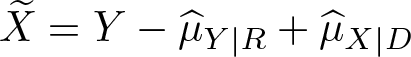
As shown by Handcock and Morris (1999), the overall relative density can be decomposed into a “location effect” and a “shape effect” by constructing a location-adjusted distribution and then using this counterfactual distribution in place of either F_X or F_Y . For example, let

$\tilde{Y}=Y-{\mu }_Y+{\mu }_X$

3

be a location-adjusted variant of Y , where µ is a location measure such as the median or the mean. In general, if $\tilde{Y}=\hspace{0.17em}t\left(Y\right)$ , the distribution of $\tilde{Y}$ is equal to $F_Y\hspace{0.17em}\left\{t^{-}{ }^1(y)\right\}$ . This means that

$F_{\tilde{Y}}(y) =P(Y-{\mu }_Y+{\mu }_X\le y) =P(Y\le y+{\mu }_Y-{\mu }_X) =F_Y(y+{\mu }_Y-{\mu }_X)$

is a location-adjusted reference distribution that has the same location as the comparison distribution. The overall relative density can then be written as

$g(r)=\frac{f_X\left\{F_Y^{-1}(r)\right\}}{f_Y\left\{F_Y^{-1}(r)\right\}}=\underset{\text{location effect }}{\underbrace{\frac{f_{\tilde{Y}}\left\{F_Y^{-1}(r)\right\}}{f_Y\left\{F_Y^{-1}(r)\right\}}}}\times \underset{\text{shape effect }}{\underbrace{\frac{f_X\left\{F_Y^{-1}(r)\right\}}{f_{\tilde{Y}}\left\{F_Y^{-1}(r)\right\}}}}$

4

The first factor, the location effect, is equal to the ratio between the density of the location-adjusted reference distribution and the unadjusted reference distribution. The second factor, the shape effect, is the ratio between the density of the (unadjusted) comparison distribution and the location-adjusted reference distribution. However, note that

$\frac{f_X\left\{F_Y^{-1}(r)\right\}}{f_{\tilde{Y}}\left\{F_Y^{-1}(r)\right\}},\hspace{1em}r\in \hspace{0.17em}[0,1]$

is not a proper density, because it is evaluated over y values distributed according to F_Y instead of $F_{\tilde{Y}}$ . It may therefore be more useful to characterize the shape effect by the adjusted relative PDF

$g_{X\tilde{Y}}(r)=\frac{f_X\left\{F_{\tilde{Y}}^{-1}(r)\right\}}{f_{\tilde{Y}}\left\{F_{\tilde{Y}}^{-1}(r)\right\}}$

or the corresponding adjusted relative CDF

$G_{X\tilde{Y}}(r)=F_X\left\{F_{\tilde{Y}}^{-1}(r)\right\}$

Instead of adjusting F_Y , the decomposition could also be defined by adjusting the comparison distribution. That is, we could use

$\tilde{X}=X-{\mu }_X+{\mu }_Y\hspace{0.17em}\text{with}\hspace{0.17em}{F}_{\tilde{X}}(y) =F_X(y+{\mu }_X-{\mu }_Y)$

such that

$g(r)=\frac{f_X\left\{F_Y^{-1}(r)\right\}}{f_Y\left\{F_Y^{-1}(r)\right\}}=\underset{\text{location effect }}{\underbrace{\frac{f_X\left\{F_Y^{-1}(r)\right\}}{f_X\left\{F_Y^{-1}(r)\right\}}}}\times \underset{\text{shape effect }}{\underbrace{\frac{f_{\tilde{X}}\left\{F_Y^{-1}(r)\right\}}{f_Y\left\{F_Y^{-1}(r)\right\}}}}$

5

As above, one of the components is not a proper density. To describe the location effect, we may thus prefer

$g_{X\tilde{X}}(r)=\frac{f_X\left\{F_{\tilde{X}}^{-1}(r)\right\}}{f_{\tilde{X}}\left\{F_{\tilde{X}}^{-1}(r)\right\}}\hspace{1em}\text{ and }\hspace{1em}{G}_{X\hspace{0.17em}\tilde{X}}(r)=F_X\left\{F_{\tilde{X}}^{-1}(r)\right\}$

instead of $f_X\left\{F_Y^{-1}(r)\right\}/f_{\tilde{X}}\left\{F_Y^{-1}(r)\right\}$ . Results from (4) and (5) will generally not be the same, although for some of the measures discussed below, it does not matter whether we adjust F_X or F_Y .

So far, an additive location shift has been used to adjust the comparison or reference distribution. For variables that can only be positive (for example, wages), it may be more natural to use a multiplicative shift and hence rescale the data proportionally. A multiplicative location adjustment of the reference distribution is given by $\tilde{Y}=Y\times {\mu }_X/{\mu }_Y$ , and hence

$F_{\tilde{Y}}(y) =F_Y(y\times {\mu }_Y/{\mu }_X)$

The comparison distribution could be adjusted analogously. Furthermore, besides the location, we could also adjust the scale of the distributions. An (additive) location and scale adjustment of the reference distribution could be accomplished using $\tilde{Y}= (Y-{\mu }_Y)\times s_X/s_Y+{\mu }_X$ , such that

$F_{\tilde{Y}}(y) =F_Y\{(y-{\mu }_X)\times s_Y/s_X+{\mu }_Y\}$

where s is a scale measure such as the interquartile range (IQR) or the standard deviation. For the multiplicative adjustment, there is no natural way to take account of the scale. However, using logarithms we can implement a proportional location and scale adjustment as $\tilde{Y}=\text{ exp}\hspace{0.17em}\left[\left\{\text{ln}(Y)-{\mu }_{\text{ln}(Y}{ }_{)}\right\}\times s_{\text{ln}(X)}/s_{\text{ln}(Y}{ }_{)}+{\mu }_{\text{ln}(X)}\right]$ , such that

$F_{\tilde{Y}}(y) =F_Y\left(\text{exp}\hspace{0.17em}\left[\{\text{ln}(y)-{\mu }_{\text{ln}(}{{ }_X}_{)}\}\times s_{\text{ln(}}{{ }_Y}_{)}/s_{\text{ln}(}{{ }_X}_{)}+{\mu }_{\text{ln(}}{{ }_Y}_{)}\right]\right)$

2.6 Summary measures

2.6.1 Divergence

Handcock and Morris (1999) suggest Pearson’s χ ² divergence and the Kullback–Leibler divergence (relative entropy) as measures for distributional divergence, that is, as summary measures for the overall difference between the comparison distribution and the reference distribution. The χ ² divergence between F_X and F_Y is defined as

${\chi }^2={\displaystyle {\int }_{-\infty }^{\infty }\frac{{\left\{f_X(y)-f_Y(y)\right\}}^2}{f_Y(y)}}\text{d}y={\displaystyle {\int }_0^1\{g(}r)-1{\}}^2 \text{d}r$

The equality between the first and second expressions follows from the substitution rule for integrals, noting that $y=F_Y^{-1}(r)\text{ and d}{F}_Y^{-1}(r)/\text{d}r=1/f_Y\left\{F_Y^{-1}(r)\right\}$ . Likewise, the Kullback–Leibler divergence, which has an information-theoretic interpretation (negative entropy of the relative density), is defined as

$\text{KL}={\displaystyle {\int }_{-\infty }^{\infty }\ln }\left\{\frac{f_X(y)}{f_Y(y)}\right\}{f}_X(y)\hspace{0.17em}\text{d}y={\displaystyle {\int }_0^1\ln }\{g(r)\}g(r)\hspace{0.17em}\text{d}r$

For both measures, the divergence of F_X with respect to F_Y is not generally equal to the divergence of F_Y with respect to F_X . That is, the direction from which we look at the problem matters. An example for a symmetric divergence measure ² is the total variation distance (TVD)

$\text{TVD}={\displaystyle {\int }_{-\infty }^{\infty }\frac{1}{2}}\hspace{0.17em}|\frac{f_X(y)}{f_Y(y)}-1|f_Y(y)\hspace{0.17em}\text{d}y={\displaystyle {\int }_0^1\frac{1}{2}}|g(r)-1|\text{d}r$

which is equal to half the area between the relative density curve and the parity line. Besides being symmetric, the TVD has an intuitive interpretation: it quantifies the proportion of data mass that would have to be redistributed in one of the distributions to make it equal to the other distribution. In the case of categorical data, the TVD is equal to the dissimilarity index by Duncan and Davis (1953), which is often used in analyses of segregation (for Stata implementations, see, for example, Jann [2004] or Reardon and Townsend [1999]).

For all three measures, in a location and shape decomposition, the location-effect divergence and the shape-effect divergence do not add up to the overall divergence. For example, we could location-adjust the reference distribution as in (3) and then obtain the location-effect divergence from $g_{\tilde{Y}}{ }_Y(r)$ and the shape-effect divergence from $g_{X\tilde{Y}}(r)$ . Unfortunately, these two divergences do not add up to the overall divergence. For the Kullback–Leibler divergence, however, as pointed out by Handcock and Morris (1999), the following equality holds:

$\text{KL}={\text{KL}}_{X\tilde{Y}Y}+{\text{KL}}_{X\tilde{Y}}$

${\text{KL}}_{X\tilde{Y}Y}$ is a (negative) cross-entropy defined as

${\text{KL}}_{X\tilde{Y}Y}={\displaystyle {\int }_{-\infty }^{\infty }\ln }\left\{\frac{f_{\tilde{Y}}(y)}{f_Y(y)}\right\}{f}_X(y)\text{d}y={\displaystyle {\int }_0^1\ln }\left\{g_{\tilde{Y}Y}(r)\right\}\hspace{0.17em}g(r)\hspace{0.17em}\text{d}r$

This suggests that, in practice, it may make sense to identify the location-effect divergence as the difference between the overall divergence and the shape-effect divergence. An advantage of such an approach is also that results will not depend on whether we adjust the reference distribution or the comparison distribution.

2.6.2 Polarization

To compare the degree of inequality between the comparison distribution and the reference distribution, Handcock and Morris (1999) suggest the median relative polarization index (MRP). The index is positive if the comparison distribution is more unequal than the reference distribution; if the reference distribution is more unequal than the comparison distribution, the index will be negative. The MRP is defined as

$\text{MRP}= 4\times E_X\left\{|r_{\tilde{Y}}(y)-0.5|\right\}-1\hspace{0.17em}\text{MRP}\in [-1,1]$

where E_X is the expectation over the comparison distribution and $r_{\tilde{Y}}(y)$ is the relative rank of y in the location-adjusted reference distribution (using the median as the location measure). The justification for the MRP is that the median of the location-adjusted relative ranks is 0.5 and the location-adjusted relative ranks will have a uniform distribution if the two distributions have the same shape. In this case, $E_X\left\{|r_{\tilde{Y}}(y)-0.5|\right\}$ is equal to 1/4, such that MRP is 0. In the extreme case that all data mass of the comparison distribution is located in regions below and above the range of the location-adjusted reference distribution, $r_{\tilde{Y}}(y)$ will be 0 or 1 for all y with positive density in F_X , such that $E_X\left\{|r_{\tilde{Y}}(y)-0.5|\right\}\hspace{0.17em}=\hspace{0.17em}0.5$ and hence MRP = 1. In the opposite extreme, $r_{\tilde{Y}}(y)$ will always be 0.5, leading to an MRP of −1.

The MRP can be decomposed into a lower polarization index (LRP) and an upper polarization index (URP) that quantify the relative polarization in the lower or upper half of the distribution, respectively:

$\begin{array}{l}\text{LRP}= 4\times E_X[abs\{r_{\tilde{Y}}(y)-0.5\}|r_{\tilde{Y}}(y)\le 0.5]-1\hfill \\ \text{URP}= 4\times E_X[abs\{r_{\tilde{Y}}(y)-0.5\}|r_{\tilde{Y}}(y)>0.5]-1\hfill \end{array}$

Because the conditional expectations in the definitions of LRP and URP each cover half the distribution of the location-adjusted relative ranks, the total polarization index is equal to the average of the lower and upper indices, that is,

$\text{MRP}= 0.5\hspace{0.17em}\times \hspace{0.17em}\text{LRP}+ 0.5\hspace{0.17em}\times \hspace{0.17em}\text{URP}$

2.6.3 Other summary measures

Descriptive statistics of the relative ranks compose a further class of relative distribution summary measures. Quantities of interest may be, for example, the mean or median of the relative ranks, their standard deviation, or their IQR.

Note that the mean of the relative ranks is equivalent to the Gastwirth index, which measures the “probability that a randomly selected woman earns at least as much as a randomly chosen man” (Gastwirth 1975, 33). ³

2.7 Covariate balancing

2.7.1 Integrating over conditional distributions

Handcock and Morris (1999) discuss covariate adjustment in terms of conditional distributions integrated over covariates. I will slightly change notation for the following exposition. Let D ∊ {0, 1} be an indicator distinguishing between a comparison group (D = 1) and a reference group (D = 0), and let Y be an outcome variable available in both groups. The comparison distribution is F_{Y | D =1}, that is, the distribution of Y in group D = 1; the reference distribution is F_{Y | D =0}. Furthermore, let Z be a continuous covariate. Our goal is to obtain the relative distribution of F_{Y | D =1} with respect to F_{Y | D =0} while adjusting for possible differences in the distribution of Z between the two groups.

The marginal distribution of Y in group d can be written as

$F_{Y\mid D=d}(y)={\displaystyle {\int }_{-\infty }^{\infty }{f}_{Z\mid D=d}}(z)F_{Y\mid D=d,Z}(y\mid z)\hspace{0.17em}\text{d}z$

where f_Z (z) is the density of Z and F_{Y | Z} (y|z) is the conditional distribution of Y given Z. A counterfactual distribution can now be constructed by replacing one of the components. For example,

$F_{Y\mid D=0}^C(y)={\displaystyle {\int }_{-\infty }^{\infty }{f}_{Z\mid D=1}}(z)F_{Y\mid D=0,Z}(y\mid z)\text{d}z$

6

is the marginal distribution of Y that we would expect in the reference group if it had the same covariate distribution as the comparison group. That is, we can obtain the counterfactual distribution by integrating the conditional distribution of Y in the reference group over the covariate distribution of the comparison group. The covariateadjusted relative distribution can then be obtained by comparing F_{Y | D =1} with $F_{Y\mid D=0\hspace{0.17em}\cdot }^C\hspace{0.17em}4$

The approach can be generalized to multiple covariates by integrating over the joint distribution of all covariates or to discrete covariates by taking weighted sums instead of integrals.

2.7.2 Reweighting

An equivalent but more attractive approach from an applied perspective is to conceptualize covariate adjustment as reweighting in the spirit of DiNardo, Fortin, and Lemieux (1996). Define

$P(D= 1|Z=z) = 1-P(D= 0|Z=z)$

as the conditional probability of belonging to the comparison group given Z. Furthermore, define

$\Psi (z)=\frac{P(D=1\mid Z=z)/P(D=1)}{P(D=0\mid Z=z)/P(D=0)}$

We can then write the counterfactual distribution of Y in the reference group as

$F_{Y\mid D=0}^C(y)={\displaystyle {\int }_{-\infty }^{\infty }{f}_{Z\mid D=0}}(z)F_{Y\mid D=0,Z}(y\mid z)\hspace{0.17em}\Psi \hspace{0.17em}(z)\hspace{0.17em}\text{d}z$

7

This indicates that the counterfactual distribution can be estimated by simply reweighting the data by an estimate of Ψ(z). ⁵ Mathematically, (7) is equivalent to (6) because

$\Psi (z)=\frac{P(D=1\mid Z=z)/P(D=1)}{P(D=0\mid Z=z)/P(D=0)}=\frac{P(D=1\mid Z=z)\times \frac{f_Z(z)}{P(D=1)}}{P(D=0\mid Z=z)\times \frac{f_Z(z)}{P(D=0)}}=\frac{f_{Z\mid D=1}(z)}{f_{Z\mid D=0}(z)}$

(using Bayes’ theorem in the last step). The practical advantage of reweighting over integrating is that Pr(D = 1|Z = z), and therefore, Ψ(z) is relatively easy to estimate using binary choice models even if Z is a vector of several covariates (for example, logistic regression). ⁶

In any case, whether we integrate over conditional distributions or we use reweighting, constructing counterfactual distributions in such a way assumes that the conditional distribution of Y is “stable”, that is, that the covariate distribution can be modified without changing the conditional distribution. However, even if such an exogeneity assumption is unrealistic in a given application, the “as if” scenarios based on counterfactual distributions can still be informative.

Furthermore, note that reweighting can be used as an alternative approach to identify location and shape effects (instead of applying adjustments as described in section 2.5) by modeling Ψ as a function of Y . This is particularly useful if the analyzed outcome is categorical.

3 Estimation

For the following discussion, assume that there is a random sample of size n for which we observe two variables, X and Y . Furthermore, there is information on sampling weights w as well as a (possibly empty) vector of covariates Z. That is, the data are (Y_i, X_i, w_i, Z_i ), i = 1,…, n. Set w_i = 1 for all i in case there are no sampling weights.

We intend to analyze the relative distribution of X with respect to Y between two subsamples. Let D be an indicator for the comparison subsample (D_i = 1 if observation i belongs to the comparison subsample, 0 if it does not), and let D = {i|D_i = 1} be the set of indices for which D_i = 1. Likewise, let R be an indicator for the reference subsample (R_i = 1 if observation i belongs to the reference subsample, 0 if it does not), and let R = {i|R_i = 1} be the set of indices for which R_i = 1. That is, we want to compare the distribution of X in subsample D with the distribution of Y in subsample R.

We will use F_{X | D} to denote the former, that is, the conditional distribution of X given D = 1, and F_{Y | R} to denote the latter. In general, we will use letter “D” for quantities related to D and letter “R” for quantities related to R. For example, $W_D={\displaystyle \sum D_i}{w}_i$ and $W_R={\displaystyle \sum R_i}{w}_i$ will be the sum of weights in the comparison sample and the reference sample, respectively. Furthermore, define $W={\displaystyle \sum w_i}$ as the total sum of weights.

Note that Y and X may be the same and that D and R do not have to be distinct nor exhaustive. I use such a general setup to cover all possible cases. For example, if the subsamples are distinct and Y = X, then we are in a setting in which a single variable is compared between two groups (for example, a comparison of wages from a sample of females to wages from a sample of males). Likewise, if D = R and Y ≠ X, we compare two variables within the same sample (for example, a comparison of data on wages for the same individuals between two time points). Furthermore, if X = Y and D is included in R, then we compare the distribution of a variable in a subsample with the pooled distribution of that variable. Finally, if the union of D and R does not cover the whole sample (that is, if there are observations for which D = R = 0), we are in a subpopulation estimation setting. Taking account of the observations that do not belong to the subpopulation may be important for standard error estimation.

3.1 The relative CDF

To obtain an estimate for the relative CDF

$G(r)=F_{X\mid D}\left\{F_{Y\mid R}^{-1}(r)\right\},\hspace{1em}r\in [0,1]$

one can compute the relative rank of X_i in distribution F_{Y | R} for each i ∊ D and then take the value of the empirical CDF of these relative ranks at value r. That is, first compute

${\widehat{r}}_i=\frac{1}{W_R}\hspace{0.17em}{\displaystyle \sum _{j\in ℛ}{w}_j}\hspace{0.17em}\mathbb{1}\left(Y_j\le X_i\right)\hspace{1em}\text{ for all }i\in \mathcal{D}$

where $\mathbb{1}$ (a) is the indicator function (1 if a is true, 0 if false). Then obtain the CDF as

$\widehat{G}(r)=\frac{1}{W_D}{\displaystyle \sum _{i\in \mathcal{D}}{w}_i\hspace{0.17em}}\mathbb{1}\left({\widehat{r}}_i\le r\right)$

8

An issue with this simple computation is that it leads to a step function with jumps at distinct values of $\widehat{r}$ . Let (i) refer to observations in D ordered by $\widehat{r}$ , such that ${\widehat{r}}_{(1)}\le {\widehat{r}}_{(2)}\le \cdots \le {\widehat{r}}_{\left(n_D\right)}. \hspace{0.17em}\text{If}\hspace{0.17em} {\widehat{r}}_{(i)}<r<{\widehat{r}}_{(i+1)}$ , that is, if evaluation point r falls between two values of $\widehat{r}$ , then $\widehat{G}(r)$ will be equal to the CDF corresponding with the lower value of $\widehat{r}$ . Such behavior makes sense in case of an ordinary CDF. However, in the context of the relative distribution, it appears more appropriate to linearly interpolate between the two points because this is equivalent to breaking ties proportionally between the comparison distribution and the reference distribution. Hence, determine $\widehat{G}(r)$ as

$\widehat{G}(r)={\widehat{G}}_{\left(i^{\prime }\right)}+\left\{{\widehat{G}}_{\left(i^{\prime }+1\right)}-{\widehat{G}}_{\left(i^{\prime }\right)}\right\}\frac{r-{\widehat{r}}_{\left(i^{\prime }\right)}}{{\widehat{r}}_{\left(i^{\prime }+1\right)}-{\widehat{r}}_{\left(i^{\prime }\right)}}$

9

with

${\widehat{G}}_{(i)}=\frac{1}{W_D}\hspace{0.17em}{\displaystyle \sum _{j\in \mathcal{D}}{w}_j}\mathbb{1}\left({\widehat{r}}_j\le {\widehat{r}}_{(i)}\right)$

where i′ is selected such that $\widehat{r}\left(i^{\prime }\right)\hspace{0.17em}<r\hspace{0.17em}\le \hspace{0.17em}\widehat{r}\hspace{0.17em}\left(i^{\prime }+1\right)$ [with ${\widehat{r}}_{(0)}={\widehat{G}}_{(0)}=0 \hspace{0.17em}if\hspace{0.17em} {\widehat{r}}_{(1)}>0$ and ${\widehat{r}}_{\left(n_D+1\right)}={\widehat{G}}_{\left(n_D+1\right)}=1\text{ if}\hspace{0.17em} {\widehat{r}}_{\left(n_D\right)}<1$ ]. For values of r that have an exact match in ${\widehat{r}}_i\hspace{0.17em},i\in D$ , this leads to the same result as (8). For r values without an exact match, (9) is equivalent to picking the result from a linear segmented curve connecting the points given by $\left\{{\widehat{G}}_{(i)},{\widehat{r}}_{(i)}\right\},i=1,\dots ,n_D$ .

Equation (9) improves on (8) in that it uses interpolation in regions where (8) is flat. It does not, however, take into account that flat regions in (8) may include outcome values that only exist in F_{Y | R} , nor does it take into account that there might be regions where the true G(r) is upright because of outcome values that only occur in F_{X | D} . To handle these issues and obtain an estimate that exactly traces the observed data pattern, we can compute the empirical CDF for F_{X | D} and F_{Y | R} at each observed value in the data and then use linear interpolation to obtain $\widehat{G}(r).\text{ Let }\mathcal{Y}=\left\{y_{(1)},\dots ,y_{(J)}\right\}$ be the ordered set of all distinct outcome values observed for F_{X | D} and F_{Y | R} . We then compute

${\widehat{r}}_{(j)}^D=\frac{1}{W_D}{\displaystyle \sum _{i\in \mathcal{D}}{w}_i}\mathbb{1}\left(X_i\le y_{(j)}\right)\hspace{1em}\text{ and }\hspace{1em}{\widehat{r}}_{(j)}^R=\frac{1}{W_R}{\displaystyle \sum _{i\in ℛ}{w}_i}\mathbb{1}\left(Y_i\le y_{(j)}\right)$

for all j = 1,…, J, add origin ${\widehat{r}}_{\left(0\right)}^D\hspace{0.17em}=\hspace{0.17em}{\widehat{r}}_{(0)}^R\hspace{0.17em}=\hspace{0.17em}0$ , and obtain the relative CDF as

$\widehat{G}(r)=\{\begin{array}{ll}{\widehat{r}}_{\left(j^r\right)}^D\hfill & \text{ if }r=0\hfill \\ {\widehat{r}}_{(jr)}^D\hfill & \text{ if }r=1\hfill \\ 0.5\left\{{\widehat{r}}_{\left(j_r\right)}^D+{\widehat{r}}_{\left(j^{\prime }\right)}^D\right\}\hfill & \text{ if }r={\widehat{r}}_{(j)}^R\text{ for any }j\hfill \\ {\widehat{r}}_{\left(j^{\prime }\right)}^D+\left\{{\widehat{r}}_{\left(j^{\prime }+1\right)}^D-{\widehat{r}}_{\left(j^{\prime }\right)}^D\right\}\hspace{0.17em}\frac{r-{\widehat{r}}_{\left(j^{\prime }\right)}^R}{{\widehat{r}}_{\left(j^{\prime }+1\right)}^R-{\widehat{r}}_{\left(j^{\prime }\right)}^R} \hspace{0.17em} \hfill & \text{else}\hfill \end{array}$

10

where j_r and j^r denote the smallest and largest value of j, respectively, for which ${\widehat{r}}_{\left(j\right)}^R\hspace{0.17em}=\hspace{0.17em}r\hspace{0.17em}$ , and where j′ is chosen such that ${\widehat{r}}_{\left(j^{\prime }\right)}^R\hspace{0.17em}<\hspace{0.17em}r\hspace{0.17em}<\hspace{0.17em}{\widehat{r}}_{\left(j^{\prime }+1\right)}^R$ . For graphical display, we may also directly plot ${\widehat{r}}_{\left(j\right)}^D$ against ${\widehat{r}}_{(j)}^R$ and linearly connect the points. All estimates for $\widehat{G}(r)$ obtained using (10) will lie on that curve.

If all values in Y exist in both distributions, (10) will lead to the same results as (9). Furthermore, for continuous data, at least if the dataset is not very small, results from the two approaches will be very similar. Equation (10), however, leads to more appropriate results than (9) if the data are discrete.

3.2 Computing relative ranks

Relative density estimation and the estimation of summary measures of the relative distribution are typically implemented by analyzing the relative ranks of X_i , i ∊ D in distribution F_{Y | R} . A naïve approach is to compute the relative ranks using the values of the empirical CDF of F_{Y | R} , that is,

${\widehat{r}}_i=\frac{1}{W_R}{\displaystyle \sum _{j\in ℛ}{w}_j}\hspace{0.17em}\mathbb{1}\left(Y_j\le X_i\right)$

11

A problem with this approach is that the empirical CDF is a step function. This is particularly troublesome if there is heaping in the data such that there are large steps in the CDF, as is often the case with discrete data. One improvement is to use the so-called middistribution function instead of the regular CDF that deducts half a step size from the ranks in regions where the CDF is upright. ⁷ Let

${\widehat{P}}_R(Y=y)=\frac{1}{W_R}{\displaystyle \sum _{j\in ℛ}{w}_j\hspace{0.17em}}\mathbb{1}\left(Y_j=y\right)$

be the relative frequency of outcome y in F_{Y | R} (that is, the step size in the CDF at value y). The relative ranks computed according to the middistribution function then are

${\widehat{r}}_i=\frac{1}{W_R}{\displaystyle \sum _{j\in ℛ}{w}_j}\hspace{0.17em}\mathbb{1}\left(Y_j\le X_i\right)-\frac{1}{2}{\widehat{P}}_R\left(Y=X_i\right)$

12

Note that (12) differs from (11) only for observations that have ties in F_{Y | R} (that is, observations that hit a step). For all other observations, ${\widehat{P}}_R$ is 0, and hence the two computations lead to the same result. The relative midranks are preferable over the naïve relative ranks because their average is exactly 0.5 if the two empirical distributions are identical. For the naïve relative ranks, this does not hold; their average will be larger than 0.5 in this situation. That is, the naïve relative ranks have an upward bias. The size of the bias depends on how much heaping there is in the data. The more heaping there is, the larger the bias.

Using the midrank adjustment removes the bias in the relative ranks. Heaping, however, will still lead to undesirable results such as arbitrary spikes in the relative density estimate. A solution to this second issue is to break ties randomly and hence smooth out the step sizes of the CDF across tied observations. These broken relative ranks (including midrank adjustment) can be written as

${\widehat{r}}_i=\frac{1}{W_R}{\displaystyle \sum _{j\in ℛ}{w}_j}1\left(Y_j\le X_i\right)-{\widehat{P}}_R\left(Y=X_i\right)\frac{{\widehat{P}}_D\left(X=X_i\right)+0.5w_i-{\delta }_i}{{\widehat{P}}_D\left(X=X_i\right)}$

13

where ${\widehat{P}}_D\hspace{0.17em}\left(X\hspace{0.17em}=\hspace{0.17em}y\right)$ is the relative frequency of outcome y in F_{X | D} and δ_i is the relative rank of X_i among all ties of X_i in F_{X | D} when ties are broken randomly. Let $w_1^{\left(i\right)}\hspace{0.17em},\mathrm{...},\hspace{0.17em}{w}_{K_i}^{\left(i\right)}$ be the randomly ordered set of weights from the observations in F_{X | D} that are equal to X_i (including observation i), where K_i is the size of the set (the order is kept stable across observations, that is, $w_k^{\left(i\right)}\hspace{0.17em},\mathrm{...},\hspace{0.17em}{w}_K^{\left(j\right)}\hspace{0.17em}\text{if}\hspace{0.17em}{X}_i=X_j$ ). Let k_i be the position of observation i in this set. The expression for δ_i then is

${\delta }_i=\frac{1}{{\displaystyle \sum _{ }^{ }{ }_{k=1}^{K_i}{w}_k^{(i)}}}{\displaystyle \sum _{k=1}^{k_i}{w}_k^{(i)}}$

which simplifies to δ_i = k_i/K_i if the weights are constant. ⁸

To obtain broken relative ranks without midrank adjustment, set 0.5w_i in (13) to 0.Whereas the midrank adjustment can have a strong effect on results if relative ranks are computed without breaking ties [(11) versus (12)], the adjustment is only of minor importance in (13) because breaking ties makes the individual step sizes small (unless there is large variation in weights).

For location-adjusted relative ranks, the same equations can be applied to appropriately transformed input variables. For example, to compute the relative ranks based on a location-adjusted reference distribution, use

$\tilde{Y}=Y-{\widehat{\mu }}_Y{{ }_{|}}_R+{\widehat{\mu }}_{X|D}$

instead of Y in the above equations, where ${\widehat{\mu }}_Y{{ }_{|}}_R$ is the median or mean of Y in subsample R and ${\widehat{\mu }}_{X|D}$ is the median or mean of X in subsample D. Location, scale, multiplicative, or logarithmic adjustments can be handled analogously.

In contrast, for shape adjustment, one of the distributions has to be swapped. For example, to compute the relative ranks based on a shape-adjusted comparison distribution (that is, a comparison distribution that has the same shape as the reference distribution but a different location), use

$\tilde{X}=Y-{\widehat{\mu }}_{Y|R}+{\widehat{\mu }}_{X|D}$

instead of X, and then set the comparison sample to $\tilde{D}=R$ instead of D.

3.3 The relative PDF

3.3.1 Kernel density estimation for continuous data

Estimation of the relative density can be implemented by applying a univariate density estimator to the relative ranks [preferably as defined in (13)]. Compared with a standard density estimation problem, there are two specific complications that should be accounted for. First, the support of the relative density is bounded at 0 and 1. Standard density estimators, however, are designed such that they smoothly approach 0 outside the support of the observed data, which leads to an underestimation of the density at the boundaries. Second, automatic bandwidth selection should be adapted to take account of the specific nature of relative data.

Given an evaluation point r ∊ [0, 1], a kernel density estimate of the relative density can be written as

$\widehat{g}(r)=\frac{1}{W_D}{\displaystyle \sum _{i\in \mathcal{D}}{w}_i}{K}_c\left(r,{\widehat{r}}_i,h\right)$

14

where $Kc\hspace{0.17em}(r, {\widehat{r}}_i, h)$ is a boundary-corrected kernel function with bandwidth h. For example, the renormalization technique uses

$K_c\left(r,{\widehat{r}}_i,h\right)=\frac{1}{h}K\left(\frac{r-{\widehat{r}}_i}{h}\right)c(r,h)\hspace{1em}\text{ with }\hspace{1em}c(r,h)={\left\{{\displaystyle {\int }_{(0-r)/h}^{(1-r)/h}K}(x)\text{d}x\right\}}^{-1}$

where K(x) is a standard kernel function such as the Gaussian kernel. The logic of the procedure is to rescale the density estimate by the inverse of the area of the kernel function that lies within the support of r. For some alternative boundary correction techniques, see Jann (2007).

The bandwidth h that determines the degree of smoothing (larger values for h lead to a smoother PDF) can either be set manually or be determined automatically from the data. Various suggestions for automatic bandwidth selectors exist in the literature, some based on crude rules of thumb and some employing more sophisticated procedures (see Jann [2007] for an overview of some of the suggestions). For relative density estimation, these standard bandwidth selectors should be adapted to take account of the specific nature of relative data. Suggestions for appropriate modifications are given by Ćwik and Mielniczuk (1993). The reldist command below supports several automatic bandwidth selectors, but we refrain from discussing their details here. ⁹

3.3.2 Histogram density estimation

A complement to kernel density estimation is to obtain a histogram of the relative density. Let (a, b ] be an interval on the support of r. The histogram density estimate for that interval can then be obtained as

$\widehat{g}(a,b)=\frac{{\widehat{P}}_D(a<r\le b)}{b-a}=\frac{1}{W_D}{\displaystyle \sum _{i\in \mathcal{D}}{w}_i}\frac{\mathbb{1}\left(a<{\widehat{r}}_i\le b\right)}{b-a}$

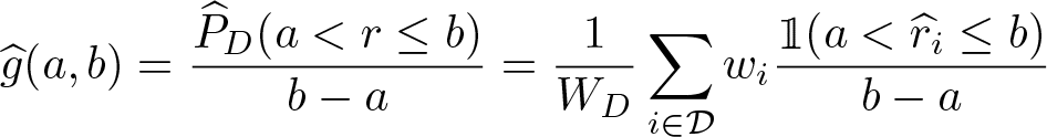
(with a modification in the case of a = 0 such that the interval includes the lower bound). A convenient setup is to split the support of r into K evenly sized bins defining the intervals $\left(0,\frac{1}{K}\right],\left(\frac{1}{K},\frac{2}{K}\right],\dots ,\left(\frac{k-1}{K},\frac{k}{K}\right],\dots ,\left(\frac{K-1}{K},1\right]$ , such that each bin covers $\frac{1}{K}$ th of the reference distribution.

The histogram density has an intuitive interpretation. For example, a value of 2 means that the fraction of the comparison distribution that falls into the bin is twice as large as the fraction of the reference distribution. In other words, the comparison distribution is overrepresented in the bin by a factor of 2. A value of 0.5 means that the proportion of the comparison distribution is only half the proportion of the reference distribution. A kernel density estimate of the relative ranks has, in principle, the same meaning (it shows the relative overrepresentation or underrepresentation multiplier at each level of r), but the explicit binning may make the histogram more easy to interpret.

3.3.3 Discrete relative density for categorical data

For categorical data, the relative density can be computed directly from the relative probabilities across the levels of the data. Without loss of generality, let k = 1,…, K be these levels. The relative density for level k is then estimated as

${\widehat{g}}_k=\frac{{\widehat{P}}_D(X=k)}{{\widehat{P}}_R(Y=k)}$

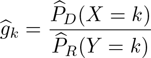
with

${\widehat{P}}_D(X=k)=\frac{1}{W_D}{\displaystyle \sum _{i\in \mathcal{D}}{w}_i}\hspace{0.17em}\mathbb{1}\left(X_i=k\right)\hspace{1em}\text{ and }\hspace{1em}{\widehat{P}}_R(Y=k)=\frac{1}{W_R}{\displaystyle \sum _{i\in ℛ}{w}_i}\hspace{0.17em}\mathbb{1}\left(Y_i=k\right)$

Discrete relative density ${\widehat{g}}_k$ is well defined only for levels k that exist in the reference distribution.

When plotting the relative density for categorical data, ${\widehat{g}}_k$ can be plotted against ${\widehat{p}}_R\hspace{0.17em}\left(Y\hspace{0.17em}\le \hspace{0.17em}k\right)\hspace{0.17em}$ using a step function, including an additional point at coordinate $\left({\widehat{g}}_1,0\right)$ for the first step. Alternatively, the density can be plotted using a histogram with bar widths equal to ${\widehat{p}}_R\hspace{0.17em}\left(Y\hspace{0.17em}=\hspace{0.17em}k\right)$ and bar midpoints equal to ${\widehat{p}}_R\hspace{0.17em}\left(Y\hspace{0.17em}\le \hspace{0.17em}k\right)\hspace{0.17em}-\hspace{0.17em}{\widehat{p}}_R\hspace{0.17em}\left(Y\hspace{0.17em}=\hspace{0.17em}k\right)\hspace{0.17em}/2$ .

3.4 Divergence

3.4.1 Continuous data

To estimate the χ ², Kullback–Leibler, and dissimilarity measures, obtain an estimate of the relative density over a grid of evaluation points and then “integrate” the result. For example, let r_k = k/K − 1/(2K), k = 1,…, K, be a regular grid of evaluation points spanning the support of r from 1/(2K) to 1 − 1/(2K). The divergence measures can then be estimated as

${\widehat{\chi }}^2=\frac{1}{K}{\displaystyle \sum _{k=1}^K{\left\{\widehat{g}\left(r_k\right)-1\right\}}^2},\hspace{1em}\widehat{\text{KL}}=\frac{1}{K}{\displaystyle \sum _{k=1}^K\widehat{g}}\left(r_k\right)\ln \left\{\widehat{g}\left(r_k\right)\right\},\hspace{1em}\widehat{\text{TVD}}=\frac{1}{2K}{\displaystyle \sum _{k=1}^K|\widehat{g}\left(r_k\right)-1|}$

15

where $\widehat{g}\hspace{0.17em}\left(r_k\right)$ is the density estimate at evaluation point r_k (that is, the integral is approximated by using a rectangle of width 1/K around each evaluation point). The size of the evaluation grid should not matter too much for the results, as long as it is sufficiently dense. However, results may strongly depend on the bandwidth used for density estimation. Divergence measures will typically increase with a decrease in the bandwidth. Stated differently, more smoothing leads to lower divergence. In general, TVD is less sensitive in this regard than the other two measures.

An alternative is to obtain the divergence measures from a histogram of the relative density. Assuming K evenly sized bins covering the whole range of r, the histogrambased estimates of the divergence measures can be obtained using (15) with $\widehat{g}\hspace{0.17em}\left(r_k\right)$ replaced by the histogram estimate of the relative density in bin k. Results may strongly depend on the number of bins.

3.4.2 Categorical data

Divergence measures for categorical data can be defined in terms of the categorical relative density as introduced above. Let k = 1,…, K be the levels of the data. The divergence estimates then are

${\widehat{\chi }}^2={\displaystyle \sum _{k=1}^K\frac{{\left({\widehat{p}}_k^D-{\widehat{p}}_k^R\right)}^2}{{\widehat{p}}_k^R}},\hspace{1em}\widehat{\text{KL}}={\displaystyle \sum _{k=1}^K{\widehat{p}}_k^D}\ln \left(\frac{{\widehat{p}}_k^D}{{\widehat{p}}_k^R}\right),\hspace{1em}\widehat{\text{TVD}}={\displaystyle \sum _{k=1}^K\frac{1}{2}}|{\widehat{p}}_k^D-{\widehat{p}}_k^R|$

where ${\widehat{p}}_k^D={\widehat{P}}_D(X=k)\text{ and }{\widehat{p}}_k^R={\widehat{P}}_R(Y=k)$ .

3.5 MRP

For the polarization indices, first compute location-adjusted relative ranks using one of the above methods, where the median is used as the location measure. Let ${\widehat{\tilde{r}}}_i$ be these location-adjusted ranks. Whether we transform the reference data or the comparison data does not matter. An estimate for MRP can then be obtained as

$\widehat{\text{MRP}}=\left(\frac{4}{W_D}{\displaystyle \sum _{i\in \mathcal{D}}{w}_i}|{\widehat{\tilde{r}}}_i-0.5|\right)-1$

Furthermore, using

$\begin{array}{l}\widehat{\text{LRP}}=\left\{\frac{8}{W_D}{\displaystyle \sum _{i\in \mathcal{D}}{w}_i}|{\widehat{\tilde{r}}}_i-0.5|\hspace{0.17em}\mathbb{1}\left({\widehat{\tilde{r}}}_i<0.5\right)\right\}-1\\ \widehat{\text{URP}}=\left\{\frac{8}{W_D}{\displaystyle \sum _{i\in \mathcal{D}}{w}_i}|{\widehat{\tilde{r}}}_i-0.5|\hspace{0.17em}\mathbb{1}\left({\widehat{\tilde{r}}}_i>0.5\right)\right\}-1\end{array}$

as estimates for LRP and URP ensures that

$\widehat{\text{MRP}}=\frac{\widehat{\text{LRP}}+\widehat{\text{URP}}}{2}$

Note that, in theory, the MRP of F_{X | D} with respect to F_{Y | R} is equal to −MRP of F_{Y | R} with respect to F_{X | D} . In practice, however, heaping in the data may cause the median of the location-adjusted relative ranks to differ from 0.5 and hence cause this relation to be violated. Applying middistribution correction and breaking ties when computing the ranks typically reduces the discrepancy but may not entirely remove it.

3.6 Covariate balancing

Assume that D and R are distinct and exhaustive, such that D is an indicator for the comparison group (D = 1) versus the reference group (D = 0). A simple approach for covariate adjustment by reweighting is to run a logistic regression of D on Z and obtain predictions ${\widehat{p}}_i=\widehat{P}\left(D=1\mid Z=Z_i\right)$ from the model. To reweight the reference group, define adjusted weights

${\tilde{w}}_i=\{\begin{array}{ll}{w}_i\frac{{\widehat{p}}_i}{1-{\widehat{p}}_i}{c}_R\hfill & \text{ if }i\in ℛ\hfill \\ w_i\hfill & \text{ else }\hfill \end{array}$

where $c_R=W_R/{\displaystyle \sum _{ }{ }_{i\in ℛ}{w}_i}\frac{{\widehat{p}}_i}{1-{\widehat{p}}_i}$ is a scaling factor ensuring that the group size (that is, its sum of weights) remains constant, and use these weights in all computations instead of the original weights. Likewise, to reweight the comparison group, define the adjusted weights as

${\tilde{w}}_i=\{\begin{array}{ll}{w}_i\frac{1-{\widehat{p}}_i}{{\widehat{p}}_i}{c}_D\hfill & \text{ if }i\in \mathcal{D}\hfill \\ w_i\hfill & \text{ else }\hfill \end{array}$

with $c_D=W_D/{\displaystyle \sum _{ }{ }_{i\in D}{w}_i}\frac{1-{\widehat{p}}_i}{{\widehat{p}}_i}$ . The described procedure is equivalent to what is known as “inverse probability weighing” (IPW) in the causal inference literature (see [TE] teffects ipw). Any other approach to obtain balancing weights may do as well. See, for example, kmatch (Jann 2017) for techniques such as entropy balancing or matching.

4 The reldist command

The command reldist implements the methods discussed above. The moremata (Jann 2005) package is required. For installation, type

4.1 Syntax

4.1.1 Estimation

The command reldist has two syntaxes. Use syntax 1 if you want to analyze the relative distribution of a single variable between two groups or subpopulations. Syntax 2 is for comparing two variables within a single sample.

Syntax 1 (two-sample relative distribution):

reldist subcmd varname [if] [in] [weight] , by( groupvar ) [options]

where groupvar identifies two groups to be compared.

Syntax 2 (paired relative distribution):

reldist subcmd varname refvar [if] [in] [weight] [ , options ]

where varname and refvar specify two variables to be compared.

In both cases, fweights, iweights, and pweights are allowed (see [U] 11.1.6 weight), and subcmd can be

4.1.2 Creating a graph after estimation

After applying reldist pdf, reldist histogram, or reldist cdf, the command reldist graph can be used to draw a graph of the results. The syntax is reldist graph , [ graph_options] An alternative is to generate the graph directly using option graph() with reldist pdf, reldist histogram, or reldist cdf.

4.1.3 Storing IFs after estimation

The command predict can be applied after reldist to generate the IFs of the estimated parameters (one variable per parameter). The syntax is

predict { stub* | newvarlist } [if] [in] [, scores density_options]

where stub specifies a common prefix for the names of the generated variables; alternatively, newvarlist specifies an explicit list of variable names to be used. Option scores is allowed for compatibility reasons; it does not do anything. density_options can be used to modify how auxiliary densities are estimated during the computation of the IFs; see page 909 for a description of available density_options (option boundary() will have no effect because unbounded support is assumed for auxiliary densities).

The command total (see [R] total) can be applied to the stored IFs to replicate the standard errors reported by reldist.

4.2 Options for reldist

4.2.1 Main options

by( groupvar ) specifies a binary variable that identifies the two groups to be compared.By default, the group with the lower value will be used as the reference group. by() is required in syntax 1 and not allowed in syntax 2.

swap reverses the order of the groups identified by by(). swap is only allowed in syntax 1. pooled uses the pooled distribution across both groups as the reference distribution.pooled is only allowed in syntax 1.

balance( spec ) balances covariate distributions between the comparison group and the reference group using reweighting. balance() is only allowed in syntax 1. The syntax of spec is [method]: varlist [, options] where method is either ipw for inverse probability weighting based on logistic regression (the default) or eb for entropy balancing (using mm_ebal() from moremata), varlist specifies the list of covariates to be balanced, and options are as follows: reference reweights the reference group. The default is to reweight the comparison group. Option pooled is not allowed with balance( varlist , reference).

contrast compares the balanced distribution with the unbalanced distribution. Use this option to see how the balancing changes the distribution. If contrast is specified together with reference, the balanced reference distribution will be used as the comparison distribution. If contrast is specified without reference, the balanced comparison distribution will be used as the reference distribution.

logit_options are options to be passed through to logit (see [R] logit). logit_options are only allowed if method is ipw.

btolerance( # ), where # ≥ 0, specifies the tolerance for the entropy balancing algorithm. The default is btolerance(1e-5). A warning message is displayed if a balancing solution is not within the specified tolerance. btolerance() is only allowed if method is eb.

noisily displays the output of the balancing procedure.

generate( newvar ) stores the balancing weights in variable newvar. This is useful if you want to check whether covariates have been successfully balanced.

adjust( spec ) applies location, scale, and shape adjustments to the comparison and reference distributions. adjust() is not allowed with reldist mrp. The syntax of spec is

adjust [, options]

where adjust specifies the desired adjustments. adjust may contain any combination of at most two of the following keywords:

location adjust location

scale adjust scale

shape adjust shape

By default, the specified adjustments are applied to the comparison distribution. However, a colon may be included in adjust to distinguish between distributions: Keywords before the colon affect the comparison distribution; keywords after the colon affect the reference distribution. For example, type adjust(location scale) to adjust the location and scale of the comparison distribution. Likewise, you could type adjust(:location scale) to adjust the reference distribution. Furthermore, adjust(location:shape) would adjust the location of the comparison distribution and the shape of the reference distribution. options are as follows:

mean uses the mean for the location adjustment. The default is to use the median. sd uses the standard deviation for the scale adjustment. The default is to use the IQR.

multiplicative uses a multiplicative adjustment instead of an additive adjustment. adjust may only contain one keyword in this case, either location or shape. An error will be returned if the location ratio between the comparison distribution and the reference distribution is not strictly positive.

logarithmic performs the adjustments on logarithmically transformed data. An error will be returned if the data are not strictly positive.

rank_options specify the details about the computation of relative ranks. These options are irrelevant for reldist histogram, reldist cdf, and reldist divergence unless option pdf is specified and for reldist pdf if discrete or categorical is specified. The options are as follows:

nobreak changes how the relative ranks are computed in case of ties. By default, reldist breaks ties randomly for comparison values that have ties in the reference distribution (in ascending order of weights if weights have been specified). This leads to improved results if there is heaping in the data. Specify nobreak to omit breaking ties.

nomid changes how the relative ranks are computed in case of ties. By default, reldist uses midpoints of the steps in the cumulative distribution for comparison values that have ties in the reference distribution. This ensures that the average relative rank is equal to 0.5 if the comparison and reference distributions are identical. Specify nomid to assign relative ranks based on full steps in the CDF.

descending sorts tied observations in descending order of weights. The default is to use ascending sort order. Option descending has no effect if nobreak is specified or if there are no weights.

nostable breaks ties randomly (within unique values of weights). The default is to break the ties in the sort order of the data (within unique values of weights). Option nostable has no effect on the results reported by reldist. It may, however, affect the ranks stored by option generate() or the IFs stored by predict (unless option nobreak is specified).

replace allows the user to replace existing variables. This is relevant for generate() with reldist summarize and generate() in balance().

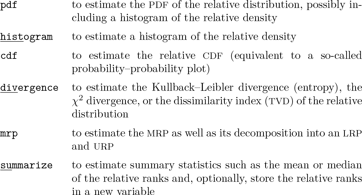
4.2.2 Additional options for reldist pdf

n( # ) sets the number of evaluation points for which the PDF is to be computed. A regular grid of # evaluation points between 0 and 1 will be used. The default is n(101) (unless option discrete or categorical is specified, in which case n() has no default). Only one of n(), at(), and atx is allowed.

at( numlist | matname ) specifies a custom grid of evaluation points between 0 and 1 by providing either a numlist (see [U] 11.1.8 numlist) or the name of a matrix containing the values (the values will be taken from the first row or the first column of the matrix, depending on which is larger). Only one of n(), at(), and atx is allowed.

atx[(comparison| reference | numlist | matname )] specified without argument causes the relative PDF to be evaluated at each distinct outcome value that exists in the data (possibly after applying adjust()), instead of using a regular evaluation grid on the probability scale. All outcome values across both distributions will be considered. To restrict the evaluation points to outcome values from the comparison distribution or the reference distribution, specify atx(comparison) or atx(reference), respectively. Alternatively, specify a grid of custom values by providing either a numlist (see [U] 11.1.8 numlist) or the name of a matrix containing the values (the values will be taken from the first row or the first column of the matrix, depending on which is larger). Only one of n(), at(), and atx is allowed.

discrete causes the data to be treated as discrete. The relative PDF will then be evaluated at each level of the data as the ratio of the level’s frequency between the comparison distribution and the reference distribution instead of using kernel density estimation, and the result will be displayed as a step function. If option n() or at() is specified, the step function will be evaluated at the points of the corresponding probability grid instead of returning the relative density for each outcome level. Options nobreak, nomid, descending, and density_options have no effect if discrete is specified. Furthermore, options histogram and adjust() are not allowed.

categorical is like discrete but additionally requests that the data only contain positive integers. Factor-variable notation will be used to label the coefficient in the output table.

histogram [( # )] computes a histogram in addition to the PDF, where # is the number of bins. If # is omitted, 10 bins will be used.

alt uses an alternative estimation method for the histogram. See the histogram options below.

density_options set the details of kernel density estimation. The options are as follows:

bwidth( # | method , nord ) determines the bandwidth of the kernel, the halfwidth of the estimation window around each evaluation point. Use bwidth( # ), # > 0, to set the bandwidth to a specific value. Alternatively, type bwidth( method ) to choose an automatic bandwidth selection method. Choices are silverman (optimal of Silverman), normalscale (normal scale rule), oversmoothed (oversmoothed rule), sjpi (Sheather–Jones solve-the-equation plugin), dpi [( # )] (Sheather–Jones direct plugin estimate, where # specifies the number of stages of functional estimation; the default is 2), or isj (diffusion estimator bandwidth). The default is bw(sjpi). See Jann (2007) for information on silverman, normalscale, oversmoothed, sjpi, and dpi. For isj, see Botev, Grotowski, and Kroese (2010).

By default, if estimating the density of the relative data, all bandwidth selectors include a correction for relative data based on Ćwik and Mielniczuk (1993). Specify suboption nord to omit the correction.

bwadjust( # ) multiplies the bandwidth by #, where # > 0. The default is bwadjust(1).

boundary( method ) sets the type of boundary correction method. Choices are renorm (renormalization method; the default), reflect (reflection method), or lc (linear combination technique). See Jann (2007) for details on boundary correction methods.

adaptive( # ) specifies the number of iterations used by the adaptive kernel density estimator. The default is adaptive(0) (nonadaptive density estimator).

kernel( kernel ) specifies the kernel function to be used. kernel may be one of epanechnikov (Epanechnikov kernel function), epan2 (alternative Epanechnikov kernel function), biweight (biweight kernel function), triweight (triweight kernel function), cosine (cosine trace), gaussian (Gaussian kernel function), parzen (Parzen kernel function), rectangle (rectangle kernel function), or triangle (triangle kernel function). The default is kernel(gaussian).

napprox( # ) specifies the grid size used by the binned approximation density estimator (and by the data-driven bandwidth selectors). The default is napprox(512).

exact causes the exact kernel density estimator to be used instead of the binned approximation estimator. The exact estimator can be slow in large datasets if the density is to be evaluated at many points.

graph [( graph_options )] displays the results in a graph. The coefficients table will be suppressed in this case (unless option table is specified). Alternatively, use reldist graph to display the graph after estimation.

ogrid( # ) sets the size of the approximation grid for outcome labels. The default is ogrid(401). The grid is stored in e(ogrid) and will be used by graph option olabel() to determine the positions of outcome labels. Type noogrid to omit the computation of the grid (no outcome labels will then be available for the graph). Option ogrid() is only allowed if the relative density is computed with respect to an evaluation grid on the probability scale. If the relative density is evaluated with respect to specific outcome values (for example, if atx is specified), the outcome labels will be obtained from the information stored in e(at).

4.2.3 Additional options for reldist histogram

n( # ) specifies the number of histogram bars. The reference distribution will be divided into # bins of equal width. That is, each bin will cover 1/#th of the reference distribution. The default is n(10).

alt uses an alternative estimation method. The default method obtains the relative histogram by computing the empirical CDF of both distributions at all values that exist in the data (across both distributions). The alternative method obtains the relative histogram based on the empirical CDF of the relative ranks. In both cases, if necessary, linear interpolation will be used to map the relative CDF to the evaluation points.

discrete causes the data to be treated as discrete. The relative density will then be evaluated at each level of the data as the ratio of the level’s frequency between the two distributions, and the width of bars will be proportional to the reference distribution. Option alt has no effect and options n() and adjust() are not allowed if discrete is specified.

categorical is like discrete but additionally requests that the data only contain positive integers. Factor-variables notation will be used to label the coefficient in the output table.

graph [( graph_options )] displays the results in a graph. The coefficients table will be suppressed in this case (unless option table is specified). Alternatively, use reldist graph to display the graph after estimation.

ogrid( # ) sets the size of the approximation grid for outcome labels. The default is ogrid(401). The grid is stored in e(ogrid) and will be used by graph option olabel() to determine the positions of outcome labels. Type noogrid to omit the computation of the grid (no outcome labels will then be available for the graph). ogrid() is not allowed together with discrete or categorical.

4.2.4 Additional options for reldist cdf

n( # ) sets the number of evaluation points for which the CDF is to be computed. A regular grid of # evaluation points between 0 and 1 will be used. The default is n(101) (unless option discrete or categorical is specified, in which case n() has no default). Only one of n(), at(), and atx is allowed.

at( numlist | matname ) specifies a custom grid of evaluation points between 0 and 1 by providing either a numlist (see [U] 11.1.8 numlist) or the name of a matrix containing the values (the values will be taken from the first row or the first column of the matrix, depending on which is larger). Only one of n(), at(), and atx is allowed.

atx[(comparison| reference | numlist | matname )] specified without argument causes the relative CDF to be evaluated at each distinct outcome value that exists in the data (possibly after applying adjust()), instead of using a regular evaluation grid on the probability scale. All outcome values across both distributions will be considered. To restrict the evaluation points to outcome values from the comparison distribution or from the reference distribution, specify atx(comparison) or atx(reference), respectively. Alternatively, specify a grid of custom values by providing either a numlist (see [U] 11.1.8 numlist) or the name of a matrix containing the values (the values will be taken from the first row or the first column of the matrix, depending on which is larger). Only one of n(), at(), and atx is allowed.

alt uses an alternative estimation method. The default method obtains the relative CDF by computing the empirical CDF of both distributions at all values that exist in the data (across both distributions). The alternative method obtains the relative CDF based on the empirical CDF of the relative ranks. In both cases, if necessary, linear interpolation will be used to map the relative CDF to the evaluation points.

discrete causes the data to be treated as discrete. The relative CDF will then be evaluated at each observed outcome value instead of using an evaluation grid on the probability scale. Option discrete leads to the same result as specifying atx. Option adjust() is not allowed if discrete is specified.

categorical is like discrete but additionally requests that the data only contain positive integers. Factor-variables notation will be used to label the coefficient in the output table.

graph [( graph_options )] displays the results in a graph. The coefficients table will be suppressed in this case (unless option table is specified). Alternatively, use reldist graph to display the graph after estimation.

ogrid( # ) sets the size of the approximation grid for outcome labels. The default is ogrid(401). The grid is stored in e(ogrid) and will be used by graph option olabel() to determine the positions of outcome labels. Type noogrid to omit the computation of the grid (no outcome labels will then be available for the graph). Option ogrid() is only allowed if the relative CDF is computed with respect to an evaluation grid on the probability scale. If the relative CDF is evaluated with respect to specific outcome values (for example, if atx is specified), the outcome labels will be obtained from the information stored in e(at).

4.2.5 Additional options for reldist divergence

over( overvar ) computes results for each subpopulation defined by the values of overvar.

entropy or kl computes the Kullback–Leibler divergence (entropy) of the relative distribution. This is the default.

chi2 or chisquared computes the χ ² divergence of the relative distribution.

tvd or dissimilarity computes the dissimilarity index (TVD) of the relative distribution.

all computes all supported divergence measures. all is equivalent to entropy chi2 tvd.

n( # ) specifies the number of histogram bars or, if option pdf is specified, the number of kernel density evaluation points used to estimate the relative distribution. The default is n(20) or, if option pdf is specified, n(100).

alt uses an alternative estimation method for the histogram. See the histogram options above.

pdf computes the divergence measures based on a kernel density estimate instead of a histogram estimate.

density_options set the details of the kernel density estimation. This is only relevant if option pdf is specified. See page 909 for available options.

discrete causes the data to be treated as discrete. The relative density will then be evaluated at each level of the data as the ratio of the level’s frequency between the two distributions. Option alt has no effect, and options n(), pdf, and adjust()

are not allowed if discrete is specified.

categorical is like discrete but additionally requests that the data only contain positive integers.

compare [( options )] estimates divergence measures for two models of the relative distribution, a main model and an alternative model, and also reports the difference between the two variants. options are balance() and adjust() as described above. balance() and adjust() specified as main options are applied to the main model; balance() and adjust() specified within compare() are applied to the alternative model.

4.2.6 Additional options for reldist mrp

over( overvar ) computes results for each subpopulation defined by the values of overvar.

multiplicative applies multiplicative location adjustment. The default is to use additive adjustment. Only one of logarithmic and multiplicative is allowed. logarithmic causes the location (and, optionally, scale) adjustment to be performed on the logarithmic scale. Only one of logarithmic and multiplicative is allowed.

scale [(sd)] adjusts the scale of the data before computing the polarization indices. If scale is specified without argument, the IQR is used; that is, the scale of the data will be adjusted such that the IQR is the same in both distributions. Specify scale(sd) to use the standard deviation instead of the IQR. scale is not allowed if multiplicative is specified.

4.2.7 Additional options for reldist summarize

over( overvar ) computes results for each subpopulation defined by the values of overvar. statistics( statnames ) specifies a space-separated list of summary statistics to be reported. The default is statistics(mean). The following summary statistics are supported:

generate( newvar ) stores the relative ranks (based on adjusted data) in variable newvar. Depending on adjust(), different observations may be filled in.

4.2.8 Variance estimation options

level( # ) specifies the confidence level, as a percentage, for confidence intervals. The default is level(95) or as set by set level (see [R] level).

vce( vcetype ) determines how standard errors and confidence intervals are computed. vcetype may be

analytic [, density_options ]

cluster clustvar [, density_options ]

svy [ svy_vcetype ] [, svy_options density_options ]

bootstrap [, bootstrap_options ]

jackknife [, jackknife_options ]

The default is vce(analytic), which computes the standard errors based on IFs. Likewise, vce(cluster clustvar ) computes IF-based standard errors allowing for intragroup correlation, where clustvar specifies to which group each observation belongs. In both cases, density_options specify how auxiliary densities are estimated during the computation of the IFs (see page 909 for details; option boundary() will have no effect because unbounded support is assumed for auxiliary densities).vce(svy) computes standard errors, taking the survey design as set by svyset (see [SVY] svyset) into account. The syntax is equivalent to the syntax of the svy prefix command (see [SVY] svy); that is, vce(svy) is reldist’s way to support the svy prefix. If svy_vcetype is set to linearized, the standard errors are estimated based on IFs; use density_options to specify the details of auxiliary density estimation in this case. For a svy_vcetype other than linearized, density_options are not allowed.

vce(bootstrap) and vce(jackknife) compute standard errors using bootstrap or jackknife, respectively (see [R] bootstrap or [R] jackknife); see [R] vce_option .

If a replication technique is used for standard error estimation (that is, vce(bootstrap), vce(jackknife), or vce(svy) with svy_vcetype other than linearized), the bandwidth used by reldist pdf will be held fixed across replications (that is, if relevant, the bandwidth will be determined upfront and then held constant). If you want to repeat the bandwidth search in each replication, use bootstrap, jackknife, or svy as a prefix command.

Simulation results suggest that the IF-based standard errors work well in most situations. They may be severely biased, however, if there is heaping in the data. Replication-based techniques may yield more valid results in this case.

nose prevents reldist from computing standard errors. This saves computer time.

4.2.9 Reporting options

citransform reports transformed confidence intervals depending on the type of reported statistics (log transform for PDF and histogram density, logit transform for CDF and descriptive statistics, and inverse hyperbolic tangent transform for polarization indices). citransform only has an effect in Stata 15 or newer.

noheader suppresses the output header.

[no] table controls the output table containing the estimated coefficients. notable suppresses display of the table; table enforces display of the table if option graph has been specified.display_options are standard reporting options such as cformat() or coeflegend; see the Reporting options in [R] Estimation options.

4.3 Options for reldist graph

4.3.1 Main graph options

refline( line_options ) specifies options to affect the rendition of the parity line. See [G] line_options .

norefline suppresses the parity line.

4.3.2 Additional options after reldist pdf

cline_options affect the rendition of the PDF line. See [G] cline_options .

histopts( options ) specifies options to affect the rendition of the histogram bars (if a histogram was computed) and the corresponding confidence spikes. options are as follows:

barlook_options affect the rendition of the histogram bars. See [G] barlook_options .

ciopts( rcap_options ) specifies options to affect the rendition of the confidence spikes of the histogram bars. See [G] rcap_options .

noci omits the confidence spikes of the histogram bars.

nohistogram omits the histogram bars.

4.3.3 Additional options after reldist histogram

barlook_options affect the rendition of the histogram bars. See [G] barlook_options .

4.3.4 Additional options after reldist cdf

noorigin prevents adding a (0, 0) coordinate to the plotted line. If the first X coordinate of the CDF is larger than 0 and the range of the CDF has not been restricted by at() or atx, reldist graph will automatically add a (0, 0) coordinate to the plot. Type noorigin to override this behavior.

cline_options affect the rendition of the CDF line. See [G] cline_options .

4.3.5 Confidence intervals

level( # ) specifies the confidence level, as a percentage, for confidence intervals. level() and ci() are not allowed together.

citransform plots transformed confidence intervals depending on the type of reported statistic (log transform for PDF and histogram density, and logit transform for CDF). ci( name ) obtains the confidence intervals from e( name ) instead of computing them from e(V). e( name ) must contain two rows and the same number of columns as e(b). For example, after bootstrap estimation, you could type ci(ci_percentile) to plot percentile confidence intervals. ci() and level() are not allowed together.

ciopts( options ) specifies options to affect the rendition of the confidence intervals. See [G] area_options , or after reldist histogram, see [G] rcap_options . Use option recast() to change the plot type used for confidence intervals. For example, type ciopts(recast(rline)) to use two lines instead of an area. noci omits the confidence intervals.

4.3.6 Outcome labels

[ y ] olabel [( spec )] adds outcome labels on a secondary axis. olabel() adds outcome labels for the reference distribution; yolabel() adds outcome labels for the comparison distribution (only allowed after reldist cdf). The syntax of spec is [# # | numlist ][, [noprune| prune( mindist )] at format(% fmt ) suboptions] # # requests that (approximately) # outcome labels be added at (approximately) evenly spaced positions; the default is #6. Alternatively, specify numlist to generate labels for given outcome values.

prune( mindist ) requests that an outcome label (but not its tick) be omitted if its distance to the preceding label is less than mindist (an exception are labels that have the same position; in such a case, the largest label will be printed). The default is prune(0.1); type prune(0) or noprune to print labels at all positions. The difference between prune(0) and noprune is that prune(0) will only print one label per position, whereas noprune prints all labels, including labels that have the same position.

at causes numlist to be interpreted as a list of probabilities for which outcome labels are to be determined. Labels obtained this way will not be pruned.

format(% fmt ) specifies the display format for the outcome labels. The default is format(%6.0g). See [D] format for available formats.

suboptions are as described in [G] axis_label_options .

Option [y]olabel may be repeated. Use suboptions add and custom to generate multiple sets of labels with different rendering; see [G] axis_label_options .

[ y ] otick( spec ) adds outcome ticks on a secondary axis. otick() adds outcome ticks for the reference distribution; yotick() adds outcome ticks for the comparison distribution (only allowed after reldist cdf). The syntax of spec is

numlist [, suboptions ]

where numlist specifies the outcome values for which ticks are to be generated and suboptions are as described in [G] axis_label_options . Option [y]otick() may be repeated. Use suboptions add and custom to generate multiple sets of ticks with different rendering; see [G] axis_label_options .

[ y ] oline( spec ) draws added lines at the positions of the specified outcome values on a secondary axis. oline() adds outcome lines for the reference distribution; yoline() adds outcome lines for the comparison distribution (only allowed after reldist cdf). The syntax of spec is numlist [, suboptions]

where numlist specifies the outcome values for which added lines be generated and suboptions are as described in [G] added_line_options . Option [y]oline() may be repeated to draw multiple sets of lines with different rendering.

[ y ] otitle( tinfo ) provides a title for the outcome scale axis; see [G] title_options . otitle() is for the reference distribution; yotitle() is for the comparison distribution (only allowed after reldist cdf).

Technical note: The positions of the outcome labels, ticks, or lines are computed from information stored by reldist in e(), either from the quantiles stored in e(ogrid) or from the values stored in e(at), depending on context. There is an undocumented command called reldist olabel that can be used to compute the positions after the relative distribution has been estimated. Use this command, for example, if you want to draw a custom graph from the stored results without applying reldist graph. The syntax is

reldist olabel [# # | numlist ][, [noprune| prune( mindist ) ] at format(% fmt )

tick( numlist ) line( numlist ) y ]

where # # or numlist specifies the (number of) values for which labels are to be generated, prune() determines the pruning (see above), at changes the meaning of the main numlist (see above), format() specifies the display format for the labels, tick() specifies values for which ticks are to be generated, line() specifies values for which added lines are to be generated, and y requests outcome labels for the Y axis of the relative CDF (only allowed after reldist cdf). reldist olabel stores the following in r():

4.3.7 General graph options

addplot( plot ) provides a way to add other plots to the generated graph. See [G] addplot_option .

twoway_options are any options other than by() documented in [G] twoway_options .

4.4 Stored results

reldist stores its results in e(), similar to official Stata’s estimation commands. See the online documentation of reldist for details.

5 Examples

5.1 Wage mobility in two eras

I illustrate some of the features of reldist by replicating an analysis of permanent wage growth from Handcock and Morris (1999, chap. 8). The data cover wages of white males from two cohorts of the National Longitudinal Survey, an “original” cohort started in 1966 and a “recent” cohort started in 1979. The variable of interest is the estimated growth in permanent wages between age 16 and age 34 (see appendix C in Handcock and Morris [1999]). The data further contain information on the achieved educational level, and there is a variable providing sampling weights. ¹⁰

Wage growth has been somewhat larger in the original cohort than in the recent cohort. The outcome variable is defined as the difference in (constant dollar) log hourly wages, so a value of 1.085 for the original cohort corresponds to a real wage growth of {exp(1.085)−1}×100 = 196%. For the recent cohort, the average is only 0.878 (141%). We can also see that inequality in wage growth has been more pronounced in the recent cohort than in the original cohort because the standard deviation of log wage gains is larger. Looking at the median and IQR instead of the mean and standard deviation leads to qualitatively similar findings.

5.1.1 The relative CDF

The relative CDF of log wage gains between the recent cohort and the original cohort can be obtained as follows, with the graph displayed in figure 0.2:

Figure 2.

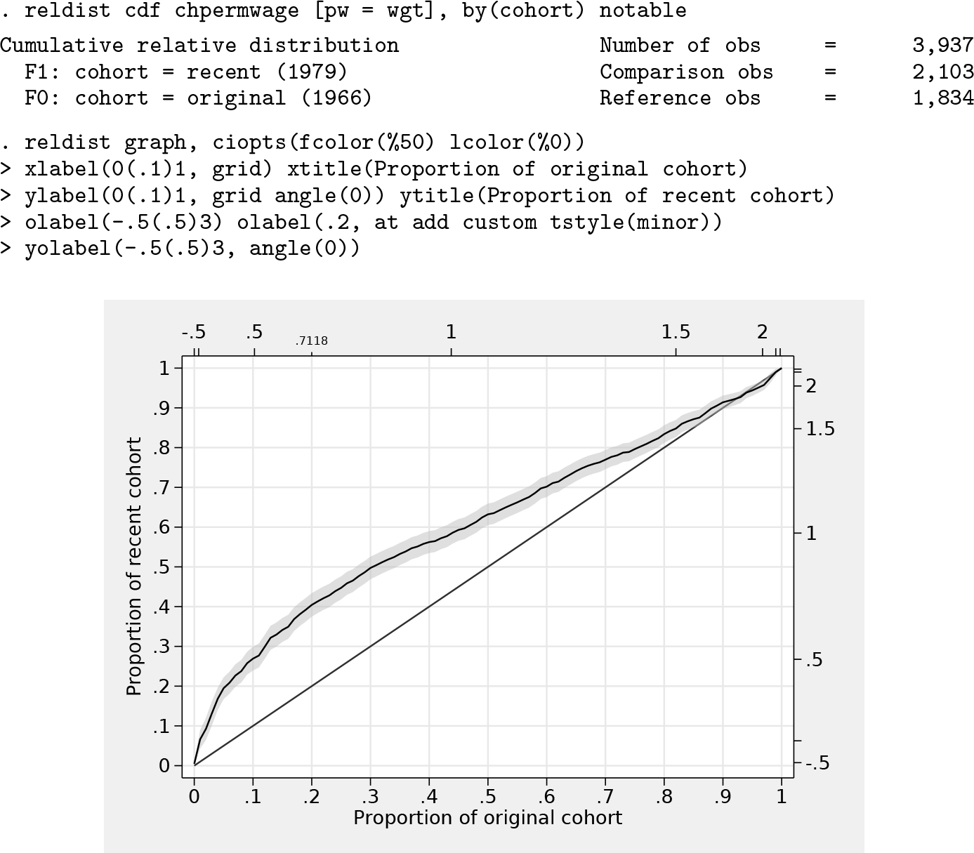
The horizontal axis of the graph corresponds to cumulative proportions of the original cohort, and the vertical axis corresponds to cumulative proportions of the recent cohort; both are ordered by the size of wage growth. Each point on the curve maps quantiles of the two distributions. For example, the value of the 20% quantile in the original cohort is equal to the 40% quantile in the recent cohort because the curve crosses point (0.2, 0.4). The 20% quantile in the original cohort corresponds to a log wage growth of 0.7118, that is, a wage growth of about 104%. In the original cohort, 20% experienced a wage growth of at most 104%; in the recent cohort, this proportion increased to 40%. That is, relative to the original cohort, wage growth of 104% or less is overrepresented by factor 2 in the recent cohort.

Comments on the used commands: Option notable has been applied to reldist cdf to suppress the output table containing the CDF estimate. By default, the CDF is evaluated at 101 points so that the table would fill a whole page. Here is an example of how the table looks if we use a reduced set of evaluation points; option at(0.1(0.1)0.9) requests 9 evaluation points located at original cohort cumulative proportions 0.1, 0.2,…, 0.9:

Coefficient p2 corresponds to cumulative proportion 0.2; as already discussed, the value of the relative CDF is about 0.4 at this point.

Furthermore, the graph has been produced by first estimating the CDF using reldist cdf and then plotting the result using reldist graph. We could also have drawn the graph in a single step by including option graph() in the call to reldist cdf (see examples farther down). Options olabel() and yolabel() have been applied to reldist graph so that additional labels are included in the graph indicating the approximate positions of specific outcome values. Labels are only printed if they are not too close together; the suppressed labels are indicated by additional ticks (this can be changed; see the description of the olabel() option above). By default, the values provided in olabel() and yolabel() are interpreted as outcome values to be included in the graph. However, if suboption at is specified, the provided values are interpreted as cumulative proportions; in this case, reldist graph will include labels for the corresponding quantiles in the graph. A second olabel() option has been used in this way in the command above to print the outcome value of the 20% quantile of the original cohort. ¹¹ Finally, option ciopts() has been added to make the confidence area transparent. The options specified within ciopts() are standard options for area plots; see [G] area_options .

5.1.2 The relative PDF

Relative overrepresentation and underrepresentation of the recent cohort with respect to the distribution of wage growth in the original cohort can be seen more directly in the relative PDF. The relative PDF can be obtained as follows, with the graph displayed in figure 3:

Figure 3.

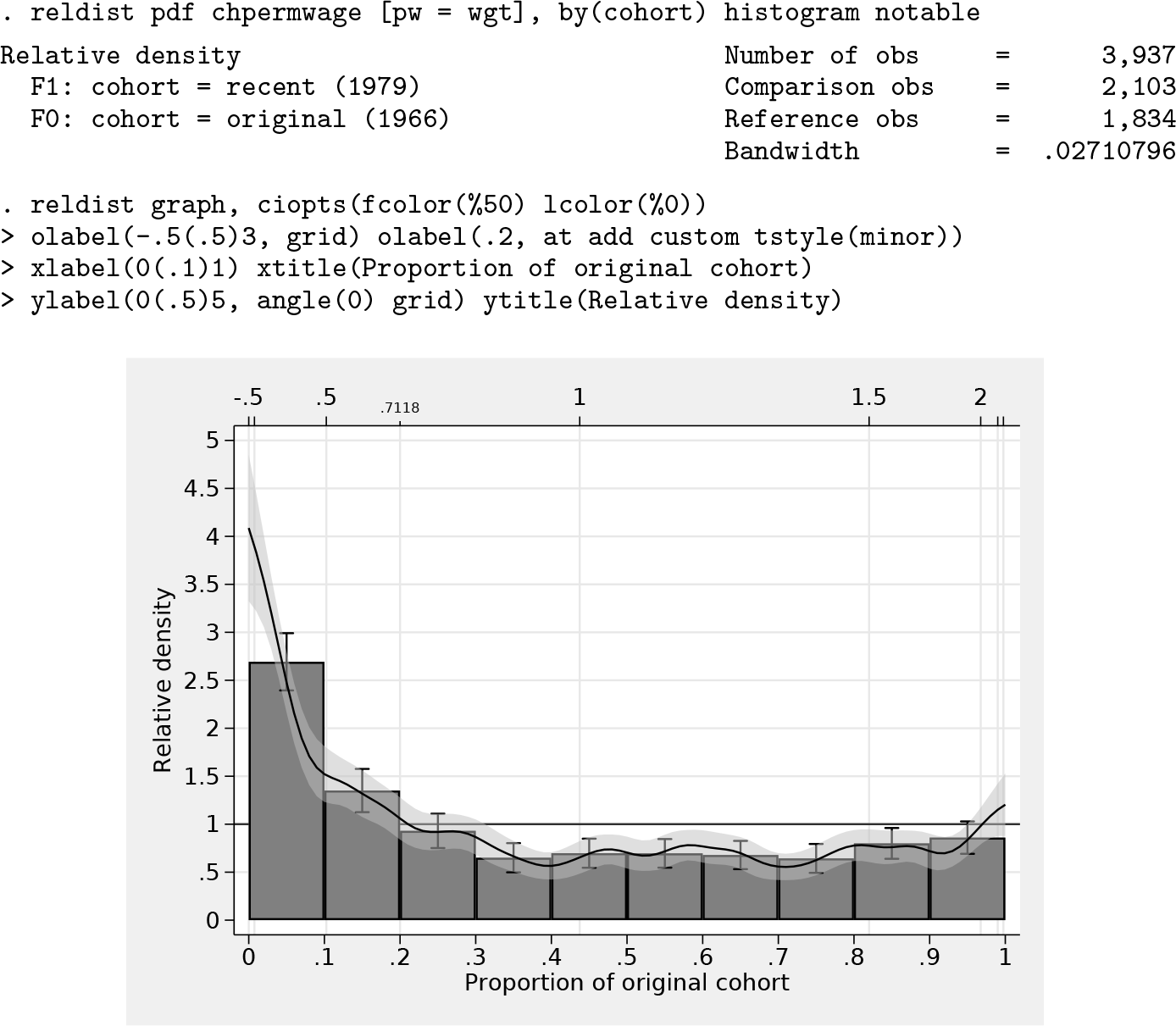
A relative density larger than 1 means the recent cohort is overrepresented at the corresponding level of wage gains, and values lower than 1 mean the recent cohort is underrepresented relative to the original cohort. We can now directly see that the largest distributional differences are at the bottom of the distribution. The recent cohort has a much larger density than the original cohort in regions below the 10% quantile of the original cohort (overrepresentation factor of 1.5 to 4) and generally a larger density below about the 20% quantile. At quantiles above that, the recent cohort is underrepresented, although there is some evidence for a reduced discrepancy at the top of the distribution (above the 80% quantile) or even a reversal at the very top (above, say, the 97% quantile; although the confidence interval includes the parity line in this region, which means that the relative density is not significantly different from 1).

5.1.3 Location and shape decomposition

The difference in the distribution of wage gains between the original cohort and the recent cohort may have various reasons. As indicated above, wage gains have been larger on average in the original cohort than in the recent cohort, which may be because of a general difference in economic growth between the two eras that affected all population members similarly. In such a case, the distribution of wage gains in the recent cohort would differ from the distribution in the original cohort only in its location. However, the structure of wage gains might also have changed, for example, because of rising returns on education, leading to more polarization of wage gains in the recent cohort. In this case, the shape of the two distributions would also be different. To separate location effects from effects of distributional differences net of location, so-called location and shape decompositions can be useful. reldist does not perform such decompositions directly, but it offers an option to obtain the relative distribution based on data that have been location- or shape-adjusted.

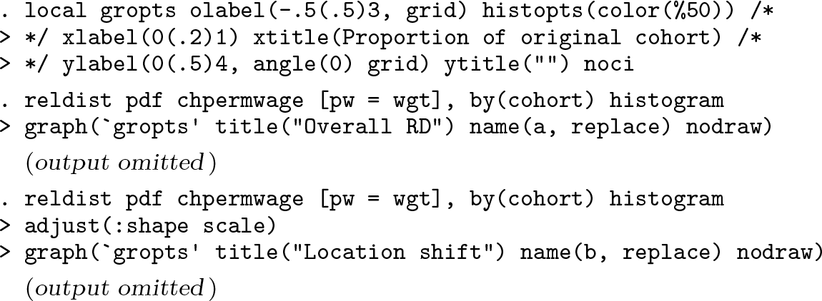
The following commands produce a graph containing three panels, shown in figure 4. ¹² The first panel shows the overall (unadjusted) relative density (same as above). The second panel shows how the relative density looks if we only allow a difference in location but keep the distributional shape fixed. This is achieved by applying option adjust(:shape scale). The option instructs reldist to adjust the original cohort distribution such that it has the same shape and scale as the recent cohort distribution but keeps its location. (Technically, this is implemented by applying a location shift to the recent cohort distribution and then replacing the original cohort distribution by this counterfactual distribution; specifying scale is necessary because, conceptually, reldist treats the scale as a separate element of a distribution that can be adjusted.) The third panel shows the relative density if the location difference between the two distributions is removed but the distributional shapes are allowed to be different. The corresponding option is adjust(location), which shifts the recent cohort distribution such that it has the same location as the original cohort distribution but keeps its shape and scale. ¹³

Figure 4.

The results indicate that the difference between the recent cohort distribution and the original cohort distribution is not only a matter of location; there is also a substantial difference in distributional shape. In particular, the recent cohort distribution appears more polarized than the original cohort (also see below).

5.1.4 Distributional divergence

To determine the relative contributions of location and shape differences to the overall distributional divergence between the two cohorts, Handcock and Morris (1999) suggest comparing the entropy (Kullback–Leibler divergence) of the unadjusted and adjusted relative distributions. Such an analysis can be obtained by reldist divergence: ¹⁴

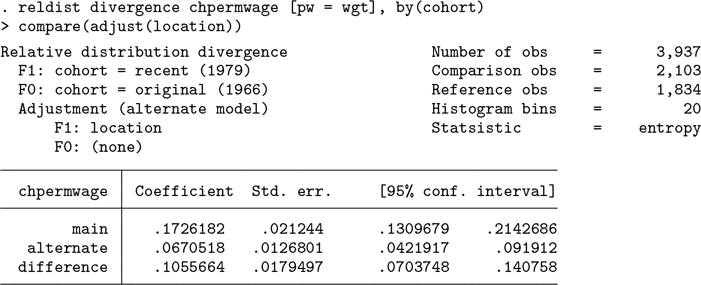
Three divergence values are reported in the above output: the divergence of the unadjusted relative distribution (labeled as main), the divergence of the relative distribution after location-adjusting the recent cohort (labeled as alternate), and the difference between these two measures. The first value is the overall divergence, the second value quantifies the divergence because of differences in distributional shape, and the third value quantifies the contribution of the difference in location. ¹⁵ We can use nlcom (see [R] nlcom) to compute the percentage contributions of the location and shape effects to the overall divergence:

We see that in this example, the difference in location appears to be more relevant (60%) than the difference in shape (40%). Qualitatively, the results are similar to the ones reported by Handcock and Morris (1999), but note that the precise values are different. Handcock and Morris performed a slightly different decomposition (see footnote 15). More importantly, however, the Kullback–Leibler divergence is quite sensitive to the details of the computation of the underlying relative density. By default, reldist divergence obtains the divergence from a 20-bin histogram; changing the number of bins may change the results substantially. Furthermore, the divergence measures could also be obtained from a kernel density estimate of the relative density (see option pdf), which would yield yet another set of results (substantially depending on the bandwidth).

5.1.5 Polarization analysis

As stated above, the recent cohort distribution appears more polarized than the original cohort distribution. A measure to quantify the polarization is the MRP computed by reldist mrp:

The results indicate that the recent cohort distribution is indeed more polarized because the value of the MRP is positive, of substantial magnitude (the possible range of the MRP is between −1 and 1), and significantly different from 0. Furthermore, the breakup into polarization of the lower half (LRP) and the upper half (URP) of the distribution suggests that the degree of relative polarization is similar in both tails.

5.1.6 Covariate balancing

Education may be one important determinant of the wage distribution as well as the distribution of wage gains over an occupational career. Hence, if the educational distribution changed between the original cohort and the recent cohort, we may be comparing apples with oranges. That is, one reason for the difference in the distribution of wage gains in the two cohorts may be that the cohorts have a different educational composition. This indeed seems to be the case if we look at the relative density of educational levels between the cohorts. ¹⁶ The resulting graph is shown in figure 5.

Figure 5.

Lower educational levels appear to be more frequent in the recent cohort than in the original cohort (relative density mostly larger than 1), and higher educational levels appear to be less frequent (relative density below 1). Looking at the table, we see that in many cases the confidence interval does not include 1, meaning that these differences between the cohorts are statistically significant.

The question now is whether these differences in educational composition affect the relative distribution of wage gains. Similarly to above in the context of location and shape effects, we can identify the contribution of compositional differences by comparing unadjusted and adjusted relative distributions. The adjustment, however, is now accomplished by reweighting one of the distributions such that its educational composition becomes equal to the educational composition in the other cohort. Option balance() can be used in reldist to apply such balancing. Here is an example (graph in figure 6) that displays the overall relative distribution (left panel), the relative distribution after the recent cohort has been reweighted (right panel), and the relative distribution between the raw and reweighted recent cohort (middle panel; the purpose of the middle panel is to show how reweighting changes the distribution of the recent cohort):

Figure 6.

Adjusting the educational composition does seem to make the distribution of wage gains somewhat more equal between the two cohorts. The comparison between the raw recent cohort and the reweighted recent cohort (middle panel) shows that low (high) wage gains are more (less) frequent in the raw data than in the reweighted data. That is, as expected, reweighting the recent cohort generally shifts the distribution of wage gains upward, thus making it more equal to the distribution of wage gains in the original cohort (the effect of the reweighting is statistically significant, as can be inferred from the confidence intervals that have been included for the histogram). Overall, however, the contribution of the difference in educational composition only seems to be of minor importance: there is only a small difference between the overall relative distribution (left panel) and the education-adjusted relative distribution (right panel).

5.1.7 Location adjustment by means of covariate balancing

Note that reweighting can be used as an alternative method for location adjustments. The default method, provided by option adjust(), implements the adjustments by transforming the outcome values. The same goal, however, can also be reached by altering the PDF of the data while leaving the outcome values unchanged. This is what reweighting does if we include the outcome variable in the balancing equation. Here is a replication of the location and shape decomposition from above using balance() instead of adjust(). I use entropy balancing to obtain the weights, which ensures that the means of the two distributions will be exactly the same. The graph is shown in figure 7.

Figure 7.

The two approaches lead to qualitatively similar results. ¹⁷ One advantage of the reweighting approach, however, is that heaping in the data will have fewer adverse effects on the results. ¹⁸

5.2 Processing results from reldist

5.2.1 Postestimation hypothesis testing

reldist stores its results in e() just like any other estimation command. Hence, we can use postestimation commands such as test (see [R] test) to test hypotheses, or we can use coefplot (Jann 2014) to draw graphs.

I use the National Longitudinal Study of Young Women 1988 data shipped with Stata to analyze wages of unionized and nonunionized workers. For example, we might be interested in relative wage polarization. An obvious hypothesis is that wages are more polarized among nonunionized workers than among the unionized, but the pattern may be different depending on education. Here are the results for the MRP between nonunionized and unionized workers for different levels of qualification:

Option swap has been specified to flip the two groups so that the nonunionized are the comparison group and the unionized are the reference group. The option multiplicative has been specified because—based on economic theory—a proportional location shift makes more sense for wages than an additive shift. As hypothesized, the results suggest that wage polarization is generally more pronounced among nonunionized workers, although the MRP is only marginally significant for respondents without a college degree. A follow-up question might thus be whether we can conclude from the data that relative polarization between nonunionized and unionized workers is stronger among college graduates than among workers without a college degree. We can use test to test the two MRP estimates against each other:

The test is negative; that is, we cannot reject the null hypothesis that the two MRP estimates are the same (p-value of 0.229). The same result could also be obtained using lincom (see [R] lincom) instead of test.

5.2.2 Creating graphs from multiple results

When comparing wages between unionized and nonunionized workers, it may be relevant to make the two groups more comparable by taking background characteristics into account. Possibly, some of the difference in the wage distributions is because of differential composition with respect to these characteristics and not because of unionization status per se. Here is how you could plot the relative density curves based on raw data and on balanced data in a single graph (figure 8) using estimates store (see [R] estimates store) and coefplot (Jann 2014):

Figure 8.

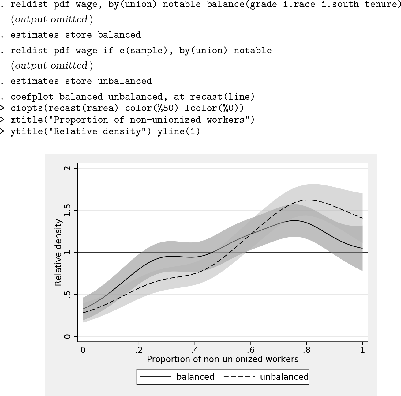
We see that the wage distributions of unionized and nonunionized workers become more similar once we control for background characteristics, especially in the upper part of the distribution.

5.2.3 Working with IFs

The predict command can be used to store the IFs that reldist uses for standard error estimation. For example, we may want to test whether relative polarization between nonunionized and unionized workers is more pronounced for wages than for working hours. reldist does not support analyzing two variables at the same time. However, we can store the IFs and then use them to test the MRP for wages against the MRP for working hours:

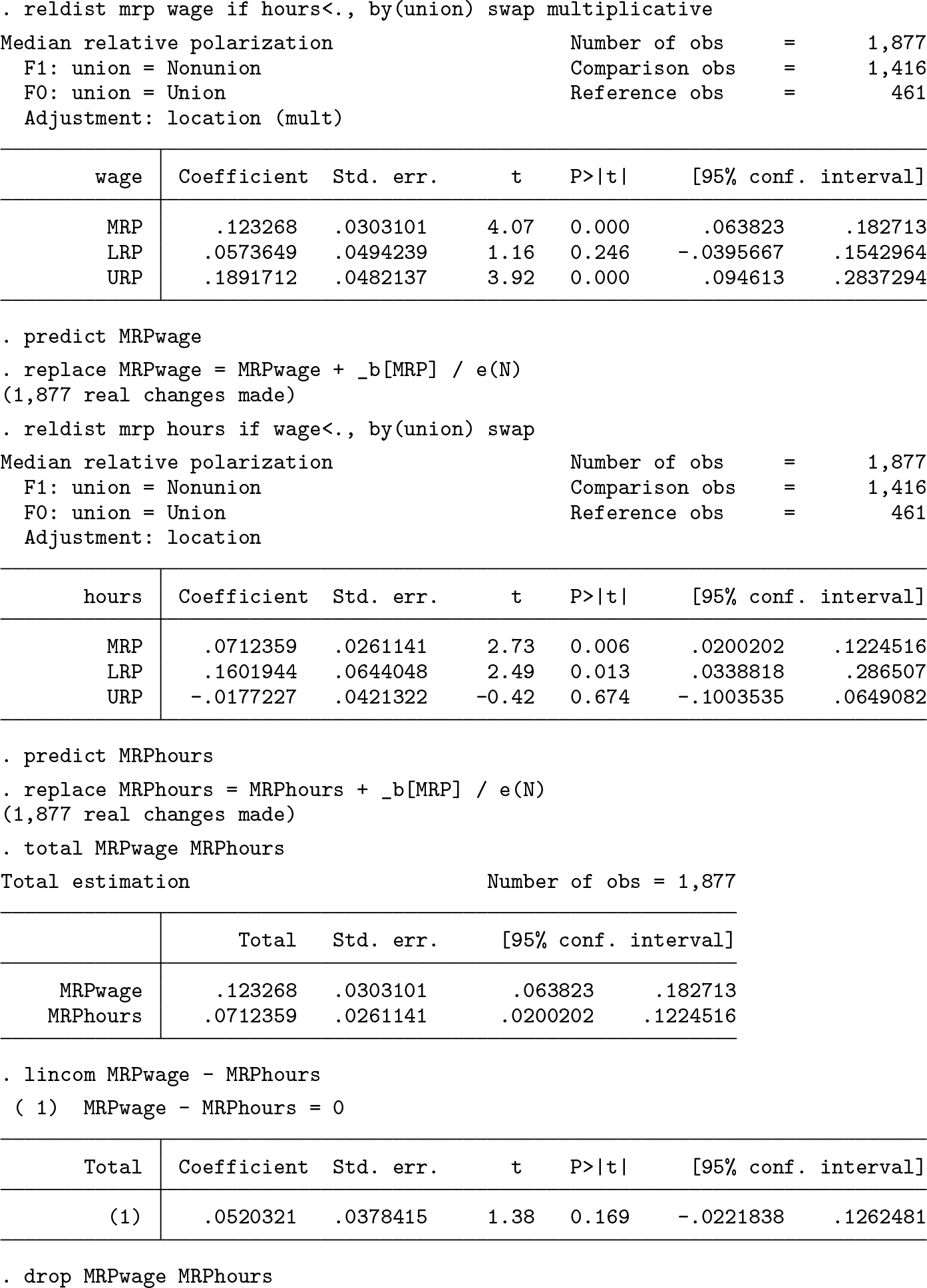
The MRP is higher for wages than for working hours, but the difference does not appear to be statistically significant. In the example, I first stored the IFs and then recentered them by adding the point estimates back in (on the use of recentered IFs, see, for example, Firpo, Fortin, and Lemieux [2009] and Rios-Avila [2020]). The IFs returned by reldist are scaled such that total (see [R] total) can be used for estimation of standard errors (note how total reproduced the results from reldist in the example).

This is why I divided the point estimate by N before adding it back in. Alternatively, multiply the IF by N, add the point estimate as is, and then use mean (see [R] mean) instead of total. Furthermore, note that weights are not incorporated into the IFs. That is, if weights have been applied to reldist, the weights will also have to be applied when calling total or mean (the same is true for clustering).

5.3 Survey estimation

reldist fully supports estimation for complex survey data, but the svy prefix command (see [SVY] svy) cannot be used for technical reasons if the variance estimation method is set to linearized(Taylor-linearized variance estimation). You can use option vce(svy) instead of the svy prefix in this case. Here is an example:

Results indicate that the birthweight distribution is somewhat less polarized for girls (childsex = 2) than for boys (childsex = 1) and that this is because of a difference in distributional shape in the upper part of the distribution (overall relative polarization is driven by the URP). Option vce(svy) also works with variance estimation methods other than linearized (for example, see [SVY] svy brr), although in these cases one could also apply svy as a prefix command. ¹⁹

7 Programs and supplemental materials

Supplemental Material, sj-zip-1-stj-10.1177_1536867X211063147 - Relative distribution analysis in Stata

Supplemental Material, sj-zip-1-stj-10.1177_1536867X211063147 for Relative distribution analysis in Stata by Ben Jann in The Stata Journal