Sage Journals: Discover world-class research

Abstract

In this article, I describe several updates to xtdcce2 (Ditzen, 2018, Stata Journal 18: 585–617). First, I explain how to estimate long-run effects in models with cross-sectional dependence. I review three methods to estimate the long-run effects and discuss their implementation into Stata using xtdcce2. Two of the estimation methods build on Chudik et al. (2016, Advances in Econometrics: Vol. 36—Essays in Honor of Aman Ullah, 85–135): the cross-sectionally augmented distributed lag and the cross-sectionally augmented autoregressive distributed lag estimator. As a third alternative, I review an error-correction model in the presence of cross-sectional dependence. Second, I explain how to estimate the exponent of cross-sectional dependence using xtcse2 following Bailey, Kapetanios, and Pesaran (2016, Journal of Applied Econometrics 31: 929–960; 2019, Sankhyā 81: 46–102).

Keywords

st0536_1 xtdcce2 xtcse2 xtcd2 parameter heterogeneity dynamic panels cross-section dependence common-correlated effects pooled mean-group estimator mean-group estimator error-correction model ardl long-run coefficients

1 Introduction

Estimation of long-run relationships is important in empirical applications of economic models, particularly macroeconomic models. Long-run relationships describe how one or more variables react to changes in the steady state. An example would be the relationships between macroeconomic variables, such as gross domestic product (GDP) and inflation. Another would be the effects of investments, exchange rates, educational progress, or technological progress on economic growth.

With pure time-series data, the autoregressive distributed lag (ARDL) model is widely used to estimate long-run relationships. ARDL models estimate the short-run coefficients and then back out the long-run coefficients. They were implemented by the communitycontributed ardl command in Stata (Kripfganz and Schneider 2018). A related model is the error-correction model (ECM). The model consists of two terms; one term captures the short-run deviations from equilibrium, and the other captures the long-run movements (Engle and Granger 1987). Both models can be applied to panel data (Pesaran and Smith 1995; Pesaran, Shin, and Smith 1999). Panel-data models add an extra layer of dimension compared with time-series models. Time-series models cover one panel unit, and slope heterogeneity across units is not an issue. Panel models include many panel units, and long- or short-run coefficients can vary across those. A popular method is the pooled mean-group (PMG) estimator, which assumes heterogeneous short-run and homogeneous long-run effects in a panel ECM (Pesaran, Shin, and Smith 1999). Blackburne and Frank (2007) implemented this method into Stata with the community-contributed command xtpmg.

The estimation of unit-specific coefficients requires datasets with many observations across time periods and cross-sectional units. Such datasets often exhibit cross-sectional dependence (CD). It implies that cross-sectional units depend on each other, for instance, by sharing a common factor. If this dependence is ignored, estimation results can be biased and inconsistent. Therefore, the extent of CD needs to be understood, and the estimation method chosen accordingly. The literature proposes two methods to identify CD. The first is to estimate the strength of the dependence (Bailey, Kapetanios, and Pesaran 2016), and the other is to test for CD (Pesaran 2015). The communitycontributed command xtcd2 (Ditzen 2018) tests for CD. This article introduces the first method, the estimation of the exponent of CD using xtcse2.

After one establishes the existence of strong CD, it can be approximated or controlled for by either principal components (Bai and Ng 2002; Bai 2009) or adding cross-sectional averages (Pesaran 2006). For a comparison, see Westerlund and Urbain (2015). Because of its simplicity, the approach using cross-sectional averages is very popular and started its own literature; Everaert and De Groote (2016), Chudik, Pesaran, and Tosetti (2011), and Chudik and Pesaran (2015a) provide overviews. The estimation method, called the common-correlated effects (CCE) estimator, applies to static (Pesaran 2006) and dynamic panel models (Chudik and Pesaran 2015b and Karabiyik, Reese, and Westerlund 2017), as well as pooled- (Juodis, Karabiyik, and Westerlund 2021) and mean-group estimators (Chudik and Pesaran 2019). The idea of the estimator is to add cross-sectional averages of the independent and dependent variables that approximate the CD. This estimator was implemented into Stata in the static version by the community-contributed command xtmg (Eberhardt 2012) and in the dynamic version by xtdcce2 (Ditzen 2018).

Neither of the commands was able to estimate long-run relationships directly. In this article, I introduce an extended version of xtdcce2 that allows the estimation of the long-run coefficients.¹ The estimation methods are based on Chudik et al. (2016) and an augmented ECM.

The remainder of the article is structured as follows. The next section introduces the panel model, CD, and CCE estimator. Then, I discuss three different methods to estimate the long-run coefficients, first from a theoretical perspective and then from an applied perspective. I give examples on how to fit the models using xtdcce2. The article closes with a conclusion.

2 Panel model and CCE estimators

For this section, assume a dynamic ARDL(1,1) panel model with heterogeneous coefficients in the form of²

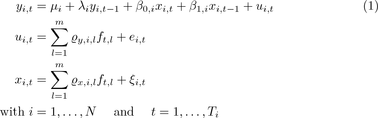
\begin{matrix} y_{i, t} = μ_{i} + λ_{i} y_{i, t - 1} + β_{0, i} x_{i, t} + β_{1, i} x_{i, t - 1} + u_{i, t} \\ u_{i, t} = \sum_{l = 1}^{m} ϱ_{y, i, l} f_{t, l} + e_{i, t} \\ x_{i, t} = \sum_{l = 1}^{m} ϱ_{x, i, l} f_{t, l} + ξ_{i, t} \\ with i = 1, \dots, N and t = 1, \dots, T_{i} \end{matrix}

where y_i,t is the dependent variable and x_i,t an observed independent variable that includes m unobserved common factors f_t,l . The estimation of the long-run effect of x on y is the main point of interest. e_i,t is a cross-section unit-specific independent and identically distributed error term. The factor loadings ϱ_x,i,l and ϱ_y,i,l are heterogeneous across units, and µ_i is a unit-specific fixed effect. The heterogeneous coefficients are randomly distributed around a common mean, such that β_i = β + v_i , and λ_i = λ + a_i , where v_i and a_i are random deviations with mean zero, independent of the error term and the common factors. λ_i lies strictly inside the unit circle to ensure a nonexplosive series.

2.1 Estimating and testing for CD

The strength of the factors can be measured by a constant 0 ≤ α ≤ 1, the so-called exponent of CD. Depending on its limiting behavior, Chudik, Pesaran, and Tosetti (2011) propose four types of CD: weak (α = 0), semiweak (0 < α < 0.5), semistrong (0.5 ≤ α < 1), and strong (α = 1) CD. (Semi)weak CD can be thought of as the following: even if the number of cross-sectional units increases to infinity, the sum of the effect of the common factors remains constant. In the case of strong CD, the sum of the effect of the common factors becomes stronger with an increase in the number of cross-sectional units.

Bailey, Kapetanios, and Pesaran (2016) propose a method for the estimation of the exponent of a variable under semistrong and strong CD. They derive a bias-adjusted estimator for α and its standard error based on auxiliary regressions using principal components and cross-sectional averages. In the case of estimating the exponent of CD in residuals, Bailey, Kapetanios, and Pesaran (2019) propose to use significant pairwise correlations of the residuals after multiple tests. A closed-form solution for standard errors is not available, and confidence intervals are constructed using a simple bootstrap. The community-contributed command xtcse2 estimates the exponent of a variable and residual.

Another possibility to determine the strength of CD is to test for (semi)weak CD (Pesaran 2015). Thus, the so-called CD test indirectly tests for α < 0.5. The test statistic is the sum across all pairwise correlations and under the null asymptotically standard normal distributed. For a further theoretical discussion of the CD test, see Pesaran (2015). The CD test is implemented in Stata by the community-contributed command xtcd2 (Ditzen 2018).

2.2 Common correlated effects estimator

Given the model in (1), leaving the factor structure unaccounted for leads to an omittedvariable bias, and ordinary least squares becomes inconsistent (Everaert and De Groote 2016). Pesaran (2006) and Chudik and Pesaran (2015b) propose an estimator to estimate (1) consistently by approximating the common factors with cross-sectional averages. In a dynamic model, the floor of $\sqrt[3]{T}$ lags of the cross-sectional averages is added. The estimated equation becomes

y_{i, t} = μ_{i} + λ_{i} y_{i, t - 1} + β_{0, i} x_{i, t} + β_{1, i} x_{i, t - 1} + \sum_{l = 0}^{p_{T}} {γ^{'}}_{i, l} {\bar{z}}_{t - l} + e_{i, t}

where ${\bar{z}}_{t} = {({\bar{y}}_{t}, {\bar{x}}_{t})}^{'} = {(1 / N \sum_{i = 1}^{N} y_{i, t}, 1 / N \sum_{i = 1}^{N} x_{i, t})}^{'}$ are the cross-sectional averages of the dependent and independent variables. γ_i,l = (γ_y,i,l, γ_x,i,l )′ are the estimated coefficients of the cross-sectional averages and are generally treated as nuisance parameters. The model can be fit by either a mean-group estimator (Pesaran and Smith 1995; Pesaran 2006; Chudik and Pesaran 2019) or a pooled estimator (Pesaran 2006; Juodis, Karabiyik, and Westerlund 2021).³ This estimator is known as the common-correlated effects mean-group (CCE-MG) estimator or CCE pooled estimator. The CCE-MG estimator is implemented in Stata by xtmg (Eberhardt 2012) and both estimators by xtdcce2 (Ditzen 2018).

3 Estimating long-run relationships

Dynamic models allow the estimation of long-run relationships. They measure the effect of an explanatory variable on the steady state value of the dependent variable. Following the notation from (1) and assuming that the model is in its steady state with $y_{t}^{*} = y_{t - 1}^{*} = y^{*}$ and $x_{t}^{*} = x_{t - 1}^{*} = x^{*}$ , we denote the long-run effect of variable x as

θ_{i} = \frac{β_{0, i} + β_{1, i}}{1 - λ_{i}}

The long-run effect in (3) can be estimated by an ARDL, distributed lag (DL), and ECM approach. All three can be augmented by cross-sectional averages to approximate CD.

3.1 CS-ECM

The cross-sectionally augmented error-correction approach (CS-ECM) follows on the lines of Lee, Pesaran, and Smith (1997) and Pesaran, Shin, and Smith (1999). Equation (2) is transformed into an ECM:⁴

Δ y_{i, t} = μ_{i} - ϕ_{i} (y_{i, t - 1} - θ_{1, i} x_{i, t}) - β_{1, i} Δ x_{i, t} + \sum_{l = 0}^{p_{T}} γ_{i, l}^{'} {\bar{z}}_{t - l} + e_{i, t}

Δ is the first-difference operator, θ_i is defined as in (3),

ϕ_{i} = (1 - λ_{i})

is the error-correction speed of the adjustment parameter, and (y_i,t− ₁ − θ _1,i x_i,t ) is the error-correction term. A long-run relationship exists if ϕ_i ≠ 0 (Pesaran, Shin, and Smith 1999). β _0,i captures the immediate or short-run effect of x_i,t on y_i,t . The long-run or equilibrium effect is captured by θ_i . The long-run effect measures how the equilibrium changes, and ϕ_i represents how fast the adjustment occurs.

In the case without CD and homogeneous long-run coefficients (θ_i = θ ∀ i), the model can be fit by the PMG estimator (Pesaran, Shin, and Smith 1999).

3.2 CS-ARDL

An alternative to the CS-ECM is the cross-sectionally augmented ARDL (CS-ARDL) approach (Chudik et al. 2016). First, the short-run coefficients are estimated, and then the long-run coefficients are calculated. The advantage of this approach is that a full set of estimates for the long- and short-run coefficients is obtained. An ARDL model can be rewritten as an ECM, and therefore the long-run estimates from the CS-ECM and CS-ARDL approaches are numerically equivalent.

Equation (1) can be generalized to an ARDL(p_y, p_x ) model:

y_{i, t} = μ_{i} + \sum_{l = 1}^{p_{_{y}}} λ_{l, i} y_{i, t - l} + \sum_{l = 0}^{p_{_{x}}} β_{l, i} x_{i, t - l} + \sum_{l = 0}^{p} {γ^{'}}_{i, l} {\bar{z}}_{t - l} + e_{i, t}

The individual long-run coefficients are calculated as

{\hat{θ}}_{CS - ARDL, i} = \frac{\sum_{l = 0}^{p_{x}} {\hat{β}}_{l, i}}{1 - \sum_{l = 1}^{p_{y}} {\hat{λ}}_{l, i}}

The coefficients can be directly estimated by the mean-group or pooled estimator. The mean-group variance estimator can be applied (Chudik et al. 2016) if the mean-group estimator is used.

3.3 CS-DL

Under the assumption that λ_i lies in the unit circle, the general representation of an ARDL(p_y, p_x ) model can be written in DL form:⁵

y_{i, t} = μ_{i} + θ_{1, i} x_{i, t} + δ_{i} (L) Δ x_{i, t} + {\tilde{u}}_{i, t}

Chudik et al. (2016) show that (5) can be directly estimated by the CCE estimator, named the cross-sectionally augmented DL (CS-DL) approach. The regression is augmented with the differences of the explanatory variables (x), their lags, and the crosssectional averages. Following Pesaran (2006), the estimation is consistent even if the errors are serially correlated.

For a general ARDL(p_y, p_x ) model with added cross-sectional averages to take out strong CD, the CS-DL estimator is based on the equation

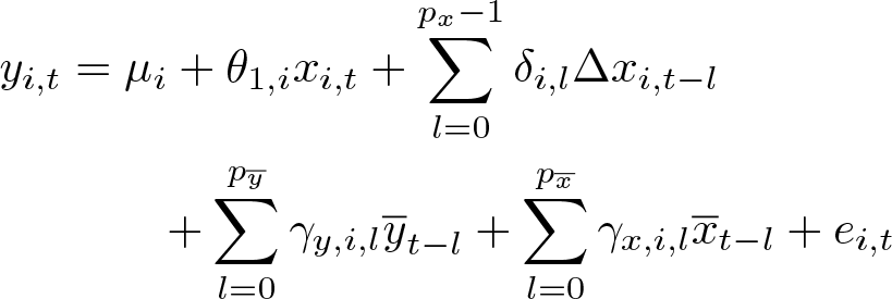
\begin{matrix} y_{i, t} = μ_{i} + θ_{1, i} x_{i, t} + \sum_{l = 0}^{p_{x} - 1} δ_{i, l} Δ x_{i, t - l} \\ + \sum_{l = 0}^{p_{\bar{y}}} γ_{y, i, l} {\bar{y}}_{t - l} + \sum_{l = 0}^{p_{\bar{x}}} γ_{x, i, l} {\bar{x}}_{t - l} + e_{i, t} \end{matrix}

where $\bar{y}$ _t−l and $\bar{x}$ _t−l are the cross-sectional averages and $p_{\bar{x}} = ⌊ T^{1 / 3} ⌋$ and $p_{\bar{y}} = 0$ .

4 Updates to the xtdcce2 command

4.1 Syntax

The updated syntax is described below. New and updated options compared with the version explained in Ditzen (2018) are described in section 4.2.

xtdcce2 depvar [ indepvars ] [ (varlist2 = varlist_iv) ] [if] [ in ] , {crosssectional( varlist_cr)| nocrosssectional} [ pooled( varlist_p) cr_lags(integers) ivreg2options(options1) e_ivreg2 ivslow noisily pooledconstant reportconstant noconstant trend pooledtrend [ jackknife| recursive ] nocd fullsample showindividual pooledvce(type) fast lr(varlist_lr) lr_options(options2) exponent xtcse2options(options3)

blockdiaguse nodimcheck useinvsym useqr noomitted showomitted ]

4.2 New and updated options

In the following, the updated or new options are explained. For a full explanation, see Ditzen (2018, 2019) and the help file for xtdcce2.

crosssectional(varlist) defines the variables that are included in z_t and added as cross-sectional averages $({\bar{z}}_{t - l})$ to the equation. Variables in crosssectional() may be included in pooled(), exogenous_vars(), endogenous_vars(), and lr(). Variables in crosssectional() are partialed out, and the coefficients are not estimated and reported.

crosssectional(_all) adds all variables as cross-sectional averages. No crosssectional averages are added if crosssectional(_none) is used, which is equivalent to nocrosssectional.

crosssectional() is required but can be substituted by nocrosssectional. nocrosssectional suppresses adding cross-sectional averages. Results will be equivalent to the Pesaran and Smith (1995) mean-group estimator or, if lr(varlist) is specified, to the Pesaran, Shin, and Smith (1999) PMG estimator. nocrosssectional cannot be specified with crosssectional().

cr_lags(integers) specifies the number of lags of the cross-sectional averages. If not defined but crosssectional() contains a varlist, then only contemporaneous crosssectional averages are added but no lags. cr_lags(0) is the equivalent. The number of lags can be different for different variables, where the order is the same as defined in crosssectional(). For example, if crosssectional(y x) and only contemporaneous cross-sectional averages of y but 2 lags of x are added, then cr_lags(0 2).

fast omits calculation of unit-specific standard errors.

lr(varlist_lr) specifies the variables to be included in the long-run cointegration vector. The first variable or variables are the error-correction speed of the adjustment term. The default is to use the PMG model. In this case, each estimated coefficient is divided by the negative of the long-run cointegration coefficient (the first variable). If the option lr_options(ardl) is used, then the long-run coefficients are estimated as the sum over the coefficients relating to a variable divided by the sum of the coefficients of the dependent variable.

lr_options(options2) specifies options for the long-run estimation. options2 may be the following:

ardl estimates the CS-ARDL estimator.

nodivide, where coefficients are not divided by the error-correction speed of the adjustment vector.

xtpmgnames, where coefficients’ names in e(b) and e(V) match the name convention from xtpmg.

exponent uses xtcse2 to estimate the exponent of the CD of the residuals. A value above 0.5 indicates strong CD.

xtcse2options(options3) passes options to xtcse2.

blockdiaguse uses the mata blockdiag option rather than an alternative algorithm.

mata blockdiag is slower but might produce more stable results.

nodimcheck does not check for dimension. Before fitting a model, xtdcce2 automatically checks whether the time dimension within each panel is long enough to run an MG regression. Panel units with an insufficient number are automatically dropped.

useinvsym calculates the generalized inverse via mata invsym.

useqr calculates the generalized inverse via QR decomposition. The default is mata cholinv. QR decomposition was the default for rank-deficient matrices for xtdcce2 preversion 1.35.

noomitted suppresses checks for collinearity.

showomitted displays a cross-sectional unit—variable breakdown of omitted coefficients.

4.2.1 New stored results

The new version stores the following two additional results:

5 The xtcse2 command

5.1 Syntax

xtcse2 [ varlist ] [ if ] [ , pca(integer) standardize nocenter nocd residual reps(integer) size(real) tuning(real) lags(integer) ]

5.2 Options

pca(integer) sets the number of principal components for the calculation of cn. The default is to use the first four components.

standardize standardizes variables.

nocenter specifies to not center variables (that is, the cross-sectional mean is zero).

nocd suppresses the test for weak CD using xtcd2.

residual estimates the exponent of CD in residuals, following Bailey, Kapetanios, and Pesaran (2019).

reps(integer) sets the number of repetitions for bootstrap for calculation of the standard error and confidence interval for the exponent in residuals. The default is reps(0).

size(real) sets the size of the test. The default is size(0.1) (10%).

tuning(real) specifies the tuning parameter for estimation of the exponent in residuals. The default is tuning(0.5).

lags(integer) specifies the number of lags (or training periods) for calculation of recursive residuals when estimating the exponent after a regression with weakly exogenous regressors.

5.3 Stored results

xtcse2 stores the following in r():

6 Empirical examples

6.1 Estimating and testing for CD

Blackburne and Frank (2007) explain the use of xtpmg by estimating the long-run consumption function from Lee, Pesaran, and Smith (1997) and Pesaran, Shin, and Smith (1999):⁶

c_{i, t} = θ_{0 t} + θ_{1 t} y_{i, t} + θ_{2 t} π_{i, t} + μ_{i} + ϵ_{i, t}

c_i,t is the log of consumption per capita, y_i,t is the log of real per capita income, and π_i,t is the inflation rate.

Before fitting the model, one must evaluate whether the variables inhibit CD. xtcse2 is used to estimate the exponent of and test for CD for the variables c_i,t (c), y_i,t (y), and π_i,t (pi):

The CD test rejects the null of weak CD for all variables, and the estimated exponent of CD is well above 0.5. This is evidence that an estimation method accounting for CD is necessary. All remaining examples are dynamic models. Following Chudik and Pesaran (2015b), the contemporaneous levels of the dependent and independent variables and the floor of T ^1/3 lags of the cross-sectional averages will be added to approximate strong CD. After each regression, the residuals are tested for strong CD using the CD test, and the exponent of CD is estimated.

6.2 CS-ECM

The ECM representation of (6) is

Δ c_{i, t} = μ_{i} - ϕ_{i} (c_{i, t - 1} - θ_{1, i} y_{i, t} - θ_{2, i} π_{i, t}) - β_{1, i} Δ y_{i, t} - β_{2, i} Δ π_{i, t} + ϵ_{i, t}

Blackburne and Frank (2007) and Ditzen (2018) fit a PMG model without and with contemporaneous cross-sectional averages using xtpmg and xtdcce2, respectively. This exercise focuses on the CS-ECM model, and all coefficients are assumed to be heterogeneous. Following Chudik and Pesaran (2015b), p = ⌊T ^1/3⌋ = ⌊29^1/3⌋ = 3 lags of the cross-sectional averages are added to be estimated (7):⁷

The mean-group estimate of the partial adjustment coefficients is $\hat{ϕ} = - 0.611$ (L.c), the long-run effect of income on consumption is ${\hat{θ}}_{1} = 0.787$ (y), and the long-run effect of inflation on consumption is ${\hat{θ}}_{2} = - 0.598$ (pi). The results imply that 61.1% of the disequilibrium is adjusted every period. An increase in income increases consumption in the long run, while an increase in prices hampers consumption in the long run.

There are some notable differences between xtpmg and xtdcce2. xtpmg calculates the long-run coefficients using maximum likelihood. xtdcce2 internally estimates (leaving out any cross-sectional averages)

Δ c_{i, t} = μ_{i} - ϕ_{i} c_{i, t - 1} + κ_{1, i} y_{i, t} + κ_{2, i} π_{i, t} - β_{1, i} Δ y_{i, t} - β_{2, i} Δ π_{i, t} + ϵ_{i, t}

using ordinary least squares with κ _1,i = −θ _1,i ϕ_i and κ _2,i = −θ _2,i ϕ_i . The long-run coefficients and the mean-group coefficients are estimated in three steps, and the variances are calculated using the delta method. First, the cross-section–specific coefficients µ_i , ϕ_i , κ _1,i, κ _2,i, β _1,i, and β _2,i are estimated. Then, the cross-section–specific long-run coefficients are calculated. Lastly, the mean-group coefficients are calculated as the unweighed average over the unit-specific long-run coefficients. As an example, the average long-run unit-specific coefficient for ${\hat{θ}}_{1, i}$ is derived as ${\hat{θ}}_{1, i} = - {\hat{κ}}_{1, i} / {\hat{ϕ}}_{i}$ . Then, the mean-group estimator is ${\hat{\bar{θ}}}_{1} = 1 / N \sum_{i = 1}^{N} {\hat{θ}}_{1, i} = 1 / N \sum_{i = 1}^{N} (- {\hat{κ}}_{1, i} / {\hat{ϕ}}_{i})$ .

The PMG estimator assumes homogeneous long-run and heterogeneous short-run coefficients. xtdcce2 is built to handle both coefficients to be heterogeneous or homogeneous. If the long-run coefficients are homogeneous but the short-run coefficients are heterogeneous, then the mean-group estimate of the error speed of the correction term is used to calculate the long-run coefficient. They then become $θ_{1}^{p} = - κ_{1}^{p} / ϕ_{MG}$ .

The option exponent is used to calculate the exponent of the CD using xtcse2. Standard errors and confidence intervals can be obtained by a simple bootstrap in which the cross-sectional units are drawn with replacement. xtdcce2 automatically runs a bootstrap with 100 repetitions. Further options to xtcse2 can be passed by the option xtcse2option(). In the example above, the p-value of the CD test is 0.79, and the test cannot reject the null hypothesis of (semi)weak CD. Bailey, Kapetanios, and Pesaran (2019, S92) state that the estimated exponent of CD should be close to 0.5 if the residuals are weakly CD. The estimated exponent of CD is 0.584 and close to the threshold of 0.5.

6.3 CS-ARDL

The ECM in (7) can be transferred into an ARDL(1,1,1) model:

c_{i, t} = μ_{i} + λ_{i} c_{i, t - 1} + β_{10, i} y_{i, t} + β_{11, i} y_{i, t - 1} + β_{20, i} π_{i, t} + β_{20, i} π_{i, t - 1} + ϵ_{i, t}

Using xtdcce2, we add all short-run variables to the lr() option and invoke the ARDL routine by using lr_options(ardl):⁸

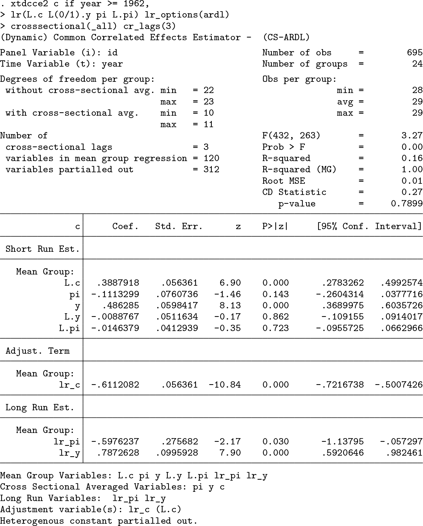
As expected, the regression results are the same as above for the CS-ECM model. In the output, the long-run coefficient estimates have the prefix lr_, and the adjustment parameter (ϕ) is displayed in a separate section. If the long-run coefficients are pooled, xtdcce2 uses the delta method to calculate the variance–covariance matrix of the longrun coefficients.

For the remaining examples, the results in Chudik et al. (2013) will be replicated. The authors estimate the long-run effect of public debt on output growth with the following equation:

Δ y_{i, t} = μ_{i} + \sum_{l = 1}^{p} λ_{i, l} Δ y_{i, t - l} + \sum_{l = 0}^{p} β_{i, l}^{'} x_{i, t - l} + \sum_{l = 0}^{3} γ_{i, l}^{'} {\bar{z}}_{t - l} + e_{i, t}

y_i,t is the logarithm of real GDP, and Δy_i,t is its growth rate. x _i,t = (Δd_i,t, π_i,t )′, d_i,t is the log of debt to GDP ratio, π is the log of the inflation rate, and p is the number of lags. The cross-sectional averages are ${\bar{z}}_{t} = ({\bar{x}}_{t}, {\bar{Δ y}}_{t})^{'}$ . The variables in the example dataset are dy for Δy_i,t , dgd for Δd_i,t , and dp for the inflation rate π_i,t .

The degree of CD is checked with

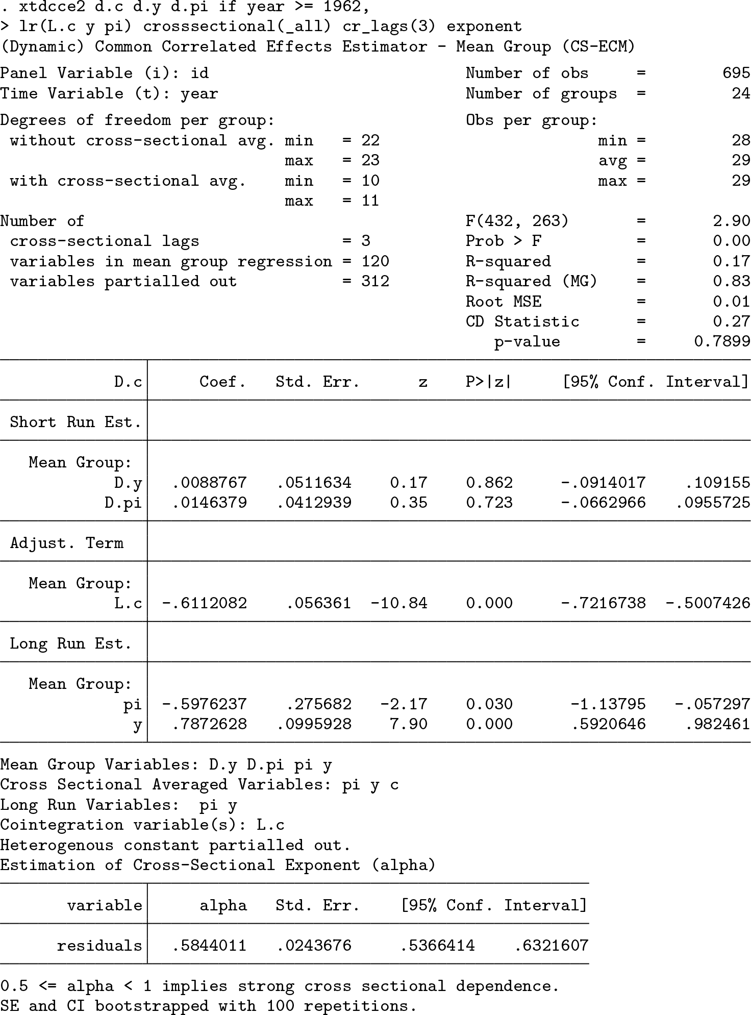
All variables are strongly CD with ${\hat{α}}_{y} = 1, {\hat{α}}_{dp} = 0.94$ , and ${\hat{α}}_{dgd} = 0.92$ . The CD test statistic yields the same conclusion: all variables contain strong CD.

Next we can turn to fit the ARDL model. As before, three lags of the cross-sectional averages are added to take out any strong CD. To replicate the results of the ARDL(1,1,1) model from Chudik et al. (2013, table 17), we add the first lag of the dependent and the base and the first lag of the dependent variables:

The long-run coefficients for the logarithm of debt to GDP ratio and inflation are both significant and negative. A decrease in the debt burden and inflation will increase GDP growth. A 1% decrease of the debt to GDP growth is associated with an increase of the GDP growth rate of 0.16%. A 1% decrease in the inflation rate leads to an increase of the GDP growth rate of 0.087%. The partial adjustment to the long-run equilibrium appears to be very quick; 95% of the gap is closed within one year.

For the ARDL(3,3,3), the three lags of the explanatory variables and the dependent variable are added. To improve readability, we enclose the different bases in parentheses:

6.4 CS-DL

Besides the ARDL model, Chudik et al. (2013) fit a CS-DL model. Equation (8) in CS-DL form is

Δ y_{i, t} = μ_{i} + θ_{i}^{'} x_{i, t} + \sum_{l = 0}^{p - 1} β_{i, l}^{'} Δ x_{i, t - l} + γ_{y, i} Δ {\bar{y}}_{t} + \sum_{l = 0}^{3} γ_{x, i, l}^{'} {\bar{x}}_{t - l} + e_{i, t}

The results from Chudik et al. (2013, table 18) with 1 lag (p = 1) in the form of an ARDL(1,1,1) model can be replicated as follows:

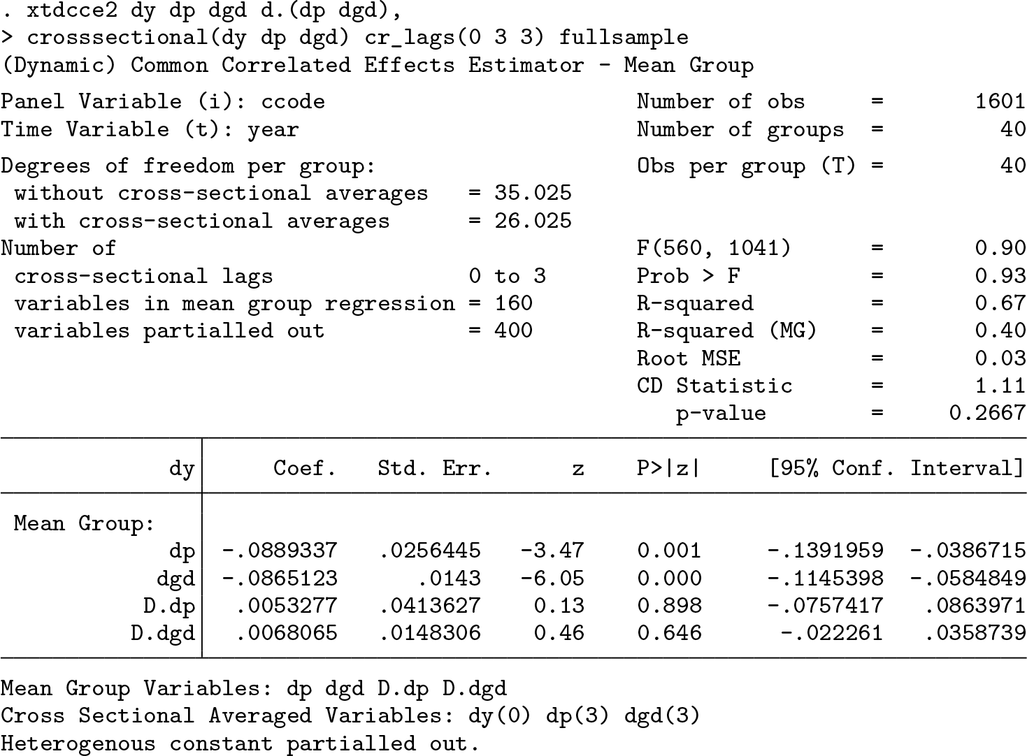
The first differences as part of the vector Δx _i,t are added as d.(dp dgd). The fullsample option is used to make use of the entire sample. The long-run coefficients are −0.0889 (dp) and −0.0865 (dgd). While the coefficient on the inflation rate is almost identical to the CS-ARDL model, the coefficient on the debt to GDP is about half the absolute size. An advantage (or disadvantage) of the CS-DL model is that no partial-adjustment coefficient is estimated, because the long-run coefficients are directly estimated.

An ARDL(3,3,3) model is fit using three rather than one lag for the differences, and L(0/2).d.(dp dgd) replaces d.(dp dgd):

The first two variables (dp and dgd) represent the long-run coefficients.

7 Conclusion

In this article, I explained how to test for CD and estimate the exponent of CD using the community-contributed command xtcse2. I then reviewed three different methods to estimate long-run coefficients in dynamic panels with many observations over time and cross-sectional units with CD. I used an extended version of xtdcce2 (Ditzen 2018) that allows for the estimation of long-run coefficients using the CS-DL, CS-ARDL, and CS-ECM estimators. Examples on how to apply xtdcce2 were given and options were explained.

Supplemental Material

Supplemental Material, sj-zip-1-stj-10.1177_1536867X211045560 - Estimating long-run effects and the exponent of cross-sectional dependence: An update to xtdcce2

Supplemental Material, sj-zip-1-stj-10.1177_1536867X211045560 for Estimating long-run effects and the exponent of cross-sectional dependence: An update to xtdcce2 by Jan Ditzen in The Stata Journal

Footnotes

8 Acknowledgments

I am grateful to all participants of the Stata User Group Meeting in Zürich in 2018 and in London in 2019, particularly Achim Ahrens and David Drukker, for valuable comments and feedback. I am grateful for help and comments from an anonymous referee and from Tore Bersvendsen, Sebastian Kripfganz, Kamiar Mohaddes, Mark Schaffer, Gregorio Tullio, and plenty of users of xtdcce2, who gave valuable feedback. xtcse2 benefited from help from Natalia Bailey and Sean Holly. All remaining errors are my own.

I acknowledge financial support from Italian Ministry MIUR under the PRIN project Hi-Di NET—Econometric Analysis of High Dimensional Models with Network Structures in Macroeconomics and Finance (grant 2017TA7TYC).

9 Programs and supplemental materials

To install a snapshot of the corresponding software files as they existed at the time of publication of this article, type

Notes

References

Bai

2009. Panel data models with interactive fixed effects. Econometrica 77: 1229–1279. https://doi.org/10.3982/ECTA6135.

Bai

2002. Determining the number of factors in approximate factor models. Econometrica 70: 191–221. https://doi.org/10.1111/1468-0262.00273.

Bailey

Kapetanios

Pesaran

M. H.

2016. Exponent of cross-sectional dependence: Estimation and inference. Journal of Applied Econometrics 31: 929–960. https://doi.org/10.1002/jae.2476.

Bailey

Kapetanios

Pesaran

M. H.

2019. Exponent of cross-sectional dependence for residuals. Sankhyā 81: 46–102. https://doi.org/10.1007/s13571-019-00196-9.

Bersvendsen

Ditzen

2020. xthst: Testing for slope homogeneity in Stata. CEERP Working Paper No. 11. https://ceerp.hw.ac.uk/RePEc/hwc/wpaper/011.pdf.

Blackburne

E. F.

III Frank

M. W.

2007. Estimation of nonstationary heterogeneous panels. Stata Journal 7: 197–208. https://doi.org/10.1177/1536867X0700700204.

Blomquist

Westerlund

2013. Testing slope homogeneity in large panels with serial correlation. Economics Letters 121: 374–378. https://doi.org/10.1016/j.econlet.2013.09.012.

Chudik

Mohaddes

Pesaran

M. H.

Raissi

2013. Debt, inflation and growth: Robust estimation of long-run effects in dynamic panel data models. Federal Reserve Bank of Dallas, Globalization and Monetary Policy Institute Working Paper No. 162. https://www.dallasfed.org/ ∼ /media/documents/institute/wpapers/2013/0162.pdf.

Chudik

Mohaddes

Pesaran

M. H.

Raissi

2016. Long-run effects in large heterogeneous panel data models with crosssectionally correlated errors. In Advances in Econometrics: Vol. 36—Essays in Honor of Aman Ullah, ed. González-Rivera

Hill

R. C.

Lee

T.-H.

, 85–135. Bingley, UK: Emerald. https://doi.org/10.1108/S0731-905320160000036013.

10.

Chudik

Pesaran

M. H.

2015a. Large panel data models with cross-sectional dependence: A survey. In The Oxford Handbook Of Panel Data, ed. Baltagi

B. H.

, 3–45. Oxford: Oxford University Press. https://doi.org/10.1093/oxfordhb/9780199940042.013.0001.

11.

Chudik

Pesaran

M. H.

2015b. Common correlated effects estimation of heterogeneous dynamic panel data models with weakly exogenous regressors. Journal of Econometrics 188: 393–420. https://doi.org/10.1016/j.jeconom.2015.03.007.

12.

Chudik

Pesaran

M. H.

2019. Mean group estimation in presence of weakly cross-correlated estimators. Economics Letters 175: 101–105. https://doi.org/10.1016/j.econlet.2018.12.036.

13.

Chudik

Pesaran

M. H.

Tosetti

2011. Weak and strong cross-section dependence and estimation of large panels. Econometrics Journal 14: C45–C90. https://doi.org/10.1111/j.1368-423X.2010.00330.x.

14.

Ditzen

2018. Estimating dynamic common-correlated effects in Stata. Stata Journal 18: 585–617. https://doi.org/10.1177/1536867X1801800306.

15.

Ditzen

2019. Estimating long run effects in models with cross-sectional dependence using xtdcce2. CEERP Working Paper No. 7. https://ceerp.hw.ac.uk/RePEc/hwc/wpaper/007.pdf.

16.

Eberhardt

2012. Estimating panel time-series models with heterogeneous slopes. Stata Journal 12: 61–71. https://doi.org/10.1177/1536867X1201200105.

17.

Engle

R. F.

Granger

C. W. J.

1987. Co-integration and error correction: Representation, estimation, and testing. Econometrica 55: 251–276. https://doi.org/10.2307/1913236.

18.

Everaert

De Groote

2016. Common correlated effects estimation of dynamic panels with cross-sectional dependence. Econometric Reviews 35: 428–463. https://doi.org/10.1080/07474938.2014.966635.

19.

Juodis

Karabiyik

Westerlund

2021. On the robustness of the pooled CCE estimator. Journal of Econometrics 220: 325–348. https://doi.org/10.1016/j.jeconom.2020.06.002.

20.

Karabiyik

Reese

Westerlund

2017. On the role of the rank condition in CCE estimation of factor-augmented panel regressions. Journal of Econometrics 197: 60–64. https://doi.org/10.1016/j.jeconom.2016.10.006.

21.

Kripfganz

Schneider

D. C.

2018. ardl: Estimating autoregressive distributed lag and equilibrium correction models. Presented September 6–7, 2018, at the Stata Conference 2018, London. https://www.stata.com/meeting/uk18/slides/uk18_Kripfganz.pdf.

22.

Lee

Pesaran

M. H.

Smith

1997. Growth and convergence in a multi-country empirical stochastic Solow model. Journal of Applied Econometrics 12: 357–392. https://doi.org/10.1002/(SICI)1099-1255(199707)12:4<357::AID-JAE441>3.0.CO;2-T.

23.

Pesaran

M. H.

2006. Estimation and inference in large heterogeneous panels with a multifactor error structure. Econometrica 74: 967–1012. https://doi.org/10.1111/j.1468-0262.2006.00692.x.

24.

Pesaran

M. H.

2015. Testing weak cross-sectional dependence in large panels. Econometric Reviews 34: 1089–1117. https://doi.org/10.1080/07474938.2014.956623.

25.

Pesaran

M. H.

Shin

Smith

R. P.

1999. Pooled mean group estimation of dynamic heterogeneous panels. Journal of the American Statistical Association 94: 621–634. https://doi.org/10.2307/2670182.

26.

Pesaran

M. H.

Smith

1995. Estimating long-run relationships from dynamic heterogeneous panels. Journal of Econometrics 68: 79–113. https://doi.org/10.1016/0304-4076(94)01644-F.

27.

Pesaran

M. H.

Yamagata

2008. Testing slope homogeneity in large panels. Journal of Econometrics 142: 50–93. https://doi.org/10.1016/j.jeconom.2007.05.010.

28.

Westerlund

Urbain

J.-P.

2015. Cross-sectional averages versus principal components. Journal of Econometrics 185: 372–377. https://doi.org/10.1016/j.jeconom.2014.09.014.

Supplementary Material

Please find the following supplemental material available below.

For Open Access articles published under a Creative Commons License, all supplemental material carries the same license as the article it is associated with.

For non-Open Access articles published, all supplemental material carries a non-exclusive license, and permission requests for re-use of supplemental material or any part of supplemental material shall be sent directly to the copyright owner as specified in the copyright notice associated with the article.

0.13 MB

0.00 MB