
Abstract
In this article, we introduce a new community-contributed command,
Keywords
1 Introduction
Today, panel data are widely used for empirical studies in several research areas, and the benefits of panel data are well known (Baltagi 2013, 6). Linear regression is undoubtedly the workhorse in empirical research, and graduate textbooks like Angrist and Pischke (2009, 86) encourage researchers to use regression models. Standard panel-data regression models like fixed effects (FEs) and random effects all assume that the parameter of interest is homogeneous. Incorrectly ignoring slope heterogeneity might bias the results; see, for example, Pesaran and Smith (1995). Whether the homogeneity assumption holds needs to be clarified before turning to the underlying empirical question.
One possibility for testing slope homogeneity is to apply the F test on the difference of the sum of squared residuals from a pooled ordinary least squares (OLS) and a cross-section unit-specific OLS regression (Baltagi 2013, 64). The main drawback from the latter test is the homoskedastic error variance assumption. In addition, the F test assumes a fixed number of cross-sectional units (N), and the test is shown to perform poorly unless T > N (Bun 2004), with T the number of time periods. Such T > N panels are relatively rare and often not used in the empirical literature. Pesaran, Smith, and Im (1996) proposed a Hausman-type test for N > T comparing the FEs estimator and cross-section unit-specific OLS, but the procedure is not applicable to panel-data models with only strictly exogenous regressors or autoregressive models (Pesaran and Yamagata 2008).
In this article, we introduce a new community-contributed command,
To our knowledge, there are two recent studies developing tests for slope heterogeneity when the errors are cross-sectional dependent. Using the same framework as Pesaran and Yamagata (2008), Ando and Bai (2015) presented a test that uses the initial idea of the interactive-effect estimator (Bai 2009). In the latter setup, the number of unknown common factors causing CSD needs to be known or estimated. Choosing a different approach, Blomquist and Westerlund (2016) developed a bootstrap-based test.
For the remainder of this article, we use the following notation: xi,t
refers to a scalar. Lowercase bold letters, such as
This article is arranged as follows. In section 2, we review and discuss the econometric theory for the different tests. In section 3, we describe the
2 Econometric theory
Consider the classical panel-data model with heterogeneous slopes

where i = 1,…, N represents the cross-sectional dimension and t = 1,…, T the time dimension. µi
is a unit-specific constant.

against the alternative:

Only coefficients in
2.1 The standard delta test
Based on a standardized version of Swamy’s (1970) test, Pesaran and Yamagata (2008) proposed a test for slope homogeneity for panel data with large N and T . The test assumes that εi,t and εj,s are independently distributed for i ≠ j or t ≠ s, or both, but allows for a heterogeneous variance. The test statistic is given by
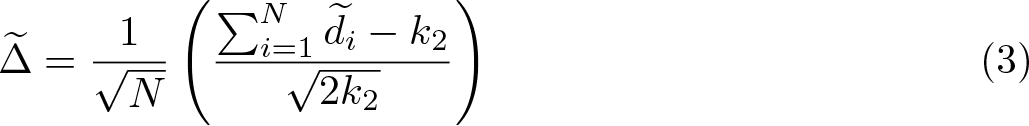
where the statistic, under H
0 in (2), is asymptotically
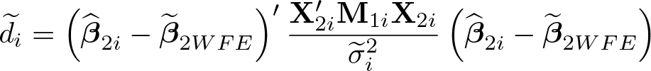
where

where

and
The regressors that are not of interest, including the constant µi
, are assumed to be heterogeneous, collected in
For normally distributed errors, the mean-variance bias-adjusted

where
2.2 A HAC robust test
Based on Pesaran and Yamagata (2008), Blomquist and Westerlund (2013) presented a HAC extension. The HAC robust test statistic is given by

where

where

where
2.3 A CSD robust test
Especially in panels with many cross-sectional units and time periods, dependence across cross-sectional units can arise. The literature differentiates between weak and strong CSD (Chudik, Pesaran, and Tosetti 2011). Weak CSD is often approximated by spatial methods. Strong CSD is modeled by a common time-specific factor ft and factor loading γi . The common factors affect all cross-sectional units,

where
When common factors and explanatory variables are correlated, leaving the factors unaccounted for leads to an omitted variable bias. Especially in the light of testing for slope heterogeneity with a test that compares the distance between the unit-specific and pooled estimator, a bias in the estimated coefficients can have a large effect. The common factors can be approximated either by principal components (Bai 2009) or by cross-sectional averages (CSA) (Pesaran 2006). The approach by Pesaran (2006), the so-called common correlated effects (CCE) estimator, has the advantage that the number of common factors does not need to be known in advance. Therefore, in the remainder, we opt for the latter technique for removing strong CSD.
Chudik and Pesaran (2015b) derive a version for weakly exogenous regressors by adding p CSA lags of the CSA and recommend setting p CSA = ⌊T 1 / 3⌋. Equation (6) with CSA would then be

where
For the CSD robust delta test, we propose to partial out the CSA to remove strong CSD from the model. Assume that matrix
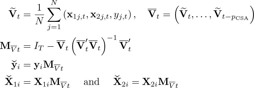
The defactored variables are then used to construct
3 The xthst command
3.1 Syntax
Data must be
depvar is the dependent variable of the model to be tested; indepvars are the independent variables. varlist_p are the variables to be partialed out; varlist_cr are variables added as CSA, calculated by
Options
Stored results

3.2 Kernel and bandwidth for the HAC robust test
Three different kernels for the estimation of the variance–covariance matrix when using the HAC robust test are built into

where scalars c and q depend on the type of kernel. When the Truncated kernel is applied, κ = 1 and
In the QS case, αi (2) follows Andrews (1991),

Applying an AR(1) model on
For the Bartlett kernel case, αi (1) is estimated according to Newey and West (1994),

where r = ⌊4(Ti/100)2
/
9⌋ and
The
4 Examples
In this section, we carry out several examples, all drawing on a growth model using the Penn World Tables 8.0 (Feenstra, Inklaar, and Timmer 2015). We restrict the dataset to 48 years between 1960 and 2007 and 93 countries. The Penn World Tables include data until 2011, but data from 2008 onward are excluded because of the financial crisis. First, we give an example for the standard
4.1 Standard
test
In this section, we want to test whether the coefficients of a cross-country growth regression are homogeneous or heterogeneous. To do so, we fit an economic growth model along the lines of Mankiw, Romer, and Weil (1992), Islam (1995), and Lee, Pesaran, and Smith (1997). The dependent variable is real gross domestic product (GDP) per capita growth in logarithms,
For a first exemplified model, we assume a static model; hence, no lag of the dependent variable occurs. We want to test whether any of the slope coefficients are homogeneous or heterogeneous. The command line and output are

In the next step, we add the first lag of GDP growth, so the regression model is an actual growth model. We extend the command line from above with
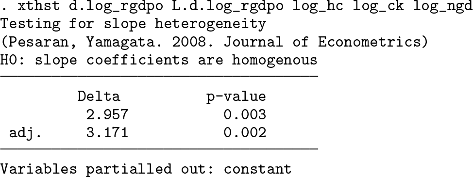
Once again, we can comfortably reject the null at a level of 5%. However, we note that the value of the test statistic decreased.
4.2 Testing a subset of coefficients
If the assumption is that all variables except the lag of GDP growth are heterogeneous, the

The test confirms that the coefficient of the lag of GDP growth is heterogeneous. The test statistic decreased in comparison with the model above.
4.3 Allowing for heteroskedastic and serially correlated errors
In a dynamic macrodataset, it is likely that errors exhibit serial correlation. To account for autocorrelation in the residual, one can use the option

The test for slope homogeneity becomes heteroskedastic robust by using a HAC robust estimator for the variance, which relies on a kernel function with a given bandwidth
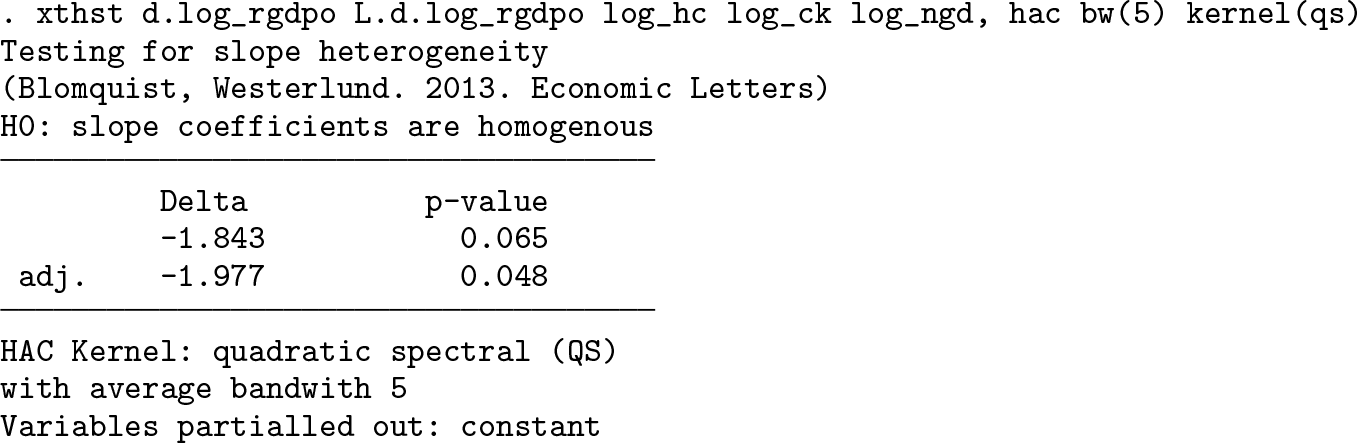
The Monte Carlo simulations in section 5 show that the performance of the delta test crucially depends on the assumption on the residuals, in particular whether autocorrelation is present. To guide the user to obtain the optimal settings, the option

In the example above, we find that the variables contain CSD that needs to be accounted for. The standard delta test and the HAC robust version lead to different results.
4.4 Accounting for CSD
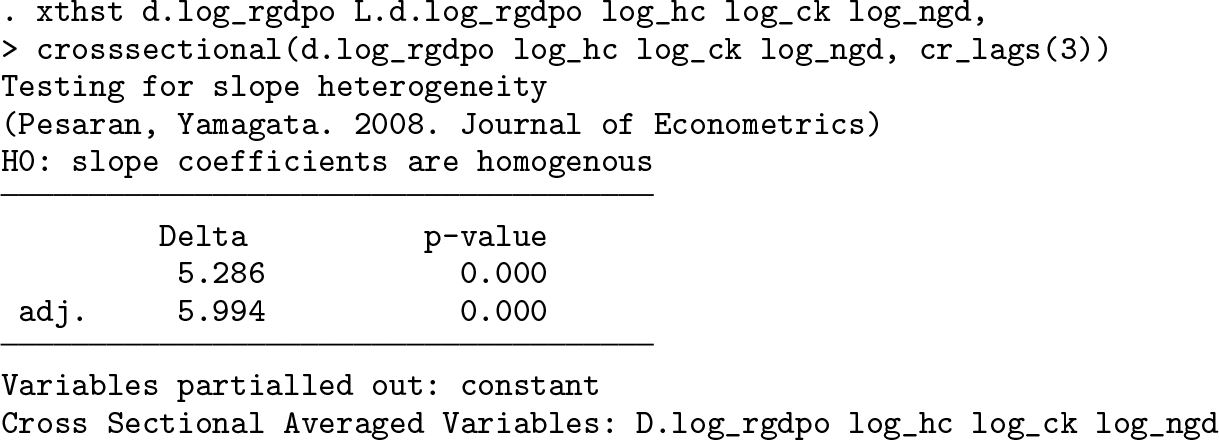
In large panels, CSD is likely, is mostly unobserved, and, if untreated, leads to biased and inconsistent regression estimates. A popular method to approximate strong CSD is to add CSA as further covariates. This estimator is known as the CCE estimator (Pesaran 2006; Chudik and Pesaran 2015b).1 In Stata, the community-contributed command
Along those lines,
We can use
5 Monte Carlo
In this section, we assess the finite sample properties using a Monte Carlo simulation. We focus on the size and the power of the delta test. The simulation setup follows Pesaran and Yamagata (2008) and Blomquist and Westerlund (2013), but we add further CSD via the independent and dependent variables.
The data-generating process (DGP) for the simulation with k regressors is

The error component ui,t contains serial correlation, if ρu,i > 0, and is heteroskedastic in all specifications. The error components of the independent and identically distributed (i.i.d.) variables, vi,t , are white noise with a unit-specific variance and are generated as

The autocorrelation coefficients of the independent variables are generated as ρx,i,l
∼ i.i.d. U(0.05, 0.95). The generation of CSD follows Chudik and Pesaran (2015b) and is introduced by the terms γx,i,lft
and γu,ift
. The common factors ft
are generated as ft
= ρf ft
−
1 +ξt
, ξt
∼ i.i.d.

where m = k is the number of regressors.
For serial correlated errors, the autocorrelation coefficients of ui,t are generated as ρu,i ∼ i.i.d. U(0, ρu ), whereas ρu is varied between 0 (no serial correlation) and 0.7 (serial correlation).
The main focus of the Monte Carlo simulation exercise will lie on the coefficient βl,i . Under the null hypothesis of homogeneous slopes, the coefficients are set to unity, βl,i = 1. Under the alternative, the first N/2 coefficients are set to unity; the remaining coefficients are drawn from a normal distribution:
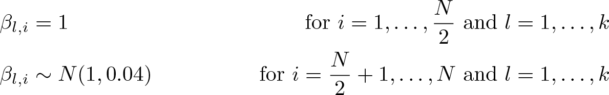
For simplicity, it is assumed that all k coefficients are the same; hence, βl,i = β 1 i . Under the alternative, the coefficients are generated as βl,i ∼ N(1, 0.04) for i > (N/2), l = 1,…, k. We vary the number of coefficients between k = 1 and k = 4. In the special case of k = 4, the first h coefficients are generated as heterogeneous even under the null hypothesis. These coefficients are then partialed out. We vary h between 0 and 1. The unit-specific FE is generated as µi ∼ N(1, 1).
In the simulations, we observe 4 cases, one without serial correlation and cross-sectional dependence (specification 1), one with either serial correlation or CSD (specifications 2 and 3), and a combination of both (specification 4). To make things easy, we focus on simulations with one regressor. Results with four regressors are available in appendix A.1 and described in more detail in Bersvendsen and Ditzen (2020).
5.1 Tests
We are comparing the results for the standard delta test
For the specification without CSD and serially correlated errors, we expect the standard delta test to perform best (specification 1 in the tables; see table 1 in appendix A.1 and sections 1–5 in figure 1). For specification 2 (sections 11–14) and specification 3 (sections 6–10), the HAC robust and CSD robust tests, respectively, should show the best size and power. Pesaran and Yamagata (2008) find that an increase in the number of regressors leads to lower performance of the tests.
5.2 Results
We present the simulation results using nested loop plots (Rücker and Schwarzer 2014). The corresponding tables can be found in appendix A.1. For all simulations, the number of cross-sectional units and time periods is varied between 20 and 200. The main focus is on the size and the power of the test. We present the size as the rejection frequencies in percent if the hypothesis is true, that is, the number of times the delta test falsely rejects the hypothesis of homogeneous slope coefficients. The power of the test is the rejection frequency if the hypothesis is false, meaning when the true coefficients are heterogeneous. The size and power are evaluated at a level of 5%.
Figure 1 displays the simulation results. The upper third of the figure shows the size, the middle the power. The different parameter settings are displayed in the lower third. For better readability, we omit the grid lines for different numbers of cross-sectional units. Each section marked with 1 to 20 represents a given parameterization with a fixed number of time periods, autocorrelation, and CSD; the number of cross-sectional units increases from 20 to 200 in each block.
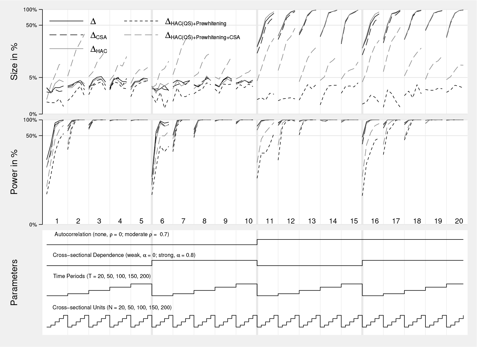
Nested loop plot of Monte Carlo simulation results. The vertical axis is scaled in logarithms. Each section, marked 1 to 20, represents a parameterization with a fixed number of time periods (T ), degree of CSD (α), and autocorrelation (ρ). The number of cross-sectional units is increased from 20 to 200. Size and power are evaluated at a level of 5%. Δ is the standard delta test, described in (3), ΔHAC is the HAC robust version from (4), ΔCSA is the CSD robust test from section 2.3. ΔHAC ( QS ) +Prewhitening is the HAC robust test with QS kernel and prewhitening, and ΔHAC ( QS ) +Prewhitening+CSA is the HAC and CSD robust test with CSA, QS kernel, and prewhitening.
In the case of no autocorrelation (sections 1–10), all tests except
When one adds CSD and no autocorrelation (sections 6–10), the standard delta test and the CSD robust delta test behave similarly for all combinations of N and T . There are two potential reasons for this. First, the CSA might take out some of the heterogeneous variation. Second, the bias of the pooled and mean group estimator is of a similar magnitude and direction. This applies to the infeasible standard OLS estimator that
Sections 11–15 show results with serially correlated errors ρu = 0.7. The standard test performs badly in terms of the size, reaching almost under 100% for all combinations of N and T . The cross-sectional robust version of the test performs somewhat better; however, it is still oversized. This result underlines the importance of a serial correlation robust version of the delta test.
The HAC robust delta test is heavily oversized; even the small-sample-adjusted test never reaches the nominal value of 5%. The equivalence holds for the power of the test. The test lacks power in small samples, especially when the number of time periods is small. However, when one uses the QS kernel with prewhitening, the HAC robust test is superior. This finding is in line with the simulation results in Blomquist and Westerlund (2013). In their simulations, the HAC robust test performs best in panels with serial correlation. Therefore, we strongly encourage users to apply this test, despite its shortcomings in size when applied to a wrong model.
The DGP in sections 16–20 contains CSD and serially correlated errors. As with serial correlation, the standard delta test and its CSD robust counterpart are oversized. The HAC robust delta with the QS kernel and prewhitening test performs surprisingly well but is slightly undersized. To encompass this, we use an additional testing procedure, ΔHAC+CSA, that first takes out strong CSD by partialing out the CSA and then uses the HAC robust delta test. While this test is oversized, the power of the test is much better than the one of the HAC robust delta test with QS kernel and prewhitening.
We present further Monte Carlo simulation results in appendix A.1 that confirm findings in Pesaran and Yamagata (2008) and Blomquist and Westerlund (2013). We find that the Bartlett kernel leads to oversized test statistics. The truncated kernel suffers from an oversize for small N and large T panels, but for large N and T panels, the size comes close to its nominal value. As found in Blomquist and Westerlund (2013), prewhitening leads to much better results for the QS kernel. Once again, the test lacks power in small samples. In general, the results strongly suggest to use the QS kernel in combination with prewhitening.
In further simulations, we extend the DGP to include four regressors. In general, the results are similar to those with only one regressor. However, the power of the tests is below those with only a single regressor. Our findings are in line with Blomquist and Westerlund (2013).
As a final exercise, we also check results with four regressors of which one is heterogeneous h = 1. Both the standard delta test and the CSD robust test have a size above their nominal value; however, in most cases, it is well below 10%. The result is expected because it is harder for the test to identify the correct heterogeneous slope coefficients. This translates into a lower power. However, for large combinations of N and T , the size and power are in acceptable regions around 5%, respectively around 90%. The oracle test, which partials out the correct variable, performs reasonably well. This implies that if a variable is known to have a heterogeneous slope parameter, partialing it out works well.
In general, the simulations confirm results established in the literature for the standard and HAC robust delta test. The correct choice of the test is crucial, and results can vary hugely. In particular, autocorrelation has a strong influence, especially on the size of the test. The extension that takes out CSD works well and can be used if CSD is suspected.
6 Conclusion
This article introduced and discussed
8 Programs and supplemental materials
Supplemental Material, sj-zip-1-stj-10.1177_1536867X211000004 - Testing for slope heterogeneity in Stata
Supplemental Material, sj-zip-1-stj-10.1177_1536867X211000004 for Testing for slope heterogeneity in Stata by Tore Bersvendsen and Jan Ditzen in The Stata Journal
Footnotes
7 Acknowledgments
We are grateful to Jochen Jungeilges for making this project possible in the first place. The article and the underlying code benefited from comments and help from Johan Blomquist, Jochen Jungeilges, Joakim Westerlund, Erich Gundlach, and an anonymous referee. We thank Tim Morris for the idea and Achim Ahrens and Jesse Wursten for comments on nested loop graphs. All remaining errors are our own.
8 Programs and supplemental materials
To install a snapshot of the corresponding software files as they existed at the time of publication of this article, type
Notes
A Appendix
References
Supplementary Material
Please find the following supplemental material available below.
For Open Access articles published under a Creative Commons License, all supplemental material carries the same license as the article it is associated with.
For non-Open Access articles published, all supplemental material carries a non-exclusive license, and permission requests for re-use of supplemental material or any part of supplemental material shall be sent directly to the copyright owner as specified in the copyright notice associated with the article.