Sage Journals: Discover world-class research

Abstract

Despite constituting a major theoretical breakthrough, the quantile selection model of Arellano and Bonhomme (2017, Econometrica 85: 1–28) based on copulas has not found its way into many empirical applications. We introduce the command arhomme, which implements different variants of the estimator along with standard errors based on bootstrapping and subsampling. We illustrate the command by replicating parts of the empirical application in the original article and a related application in Arellano and Bonhomme (2018, Handbook of Quantile Regression, chap. 13).

Keywords

st0648 arhomme Arellano and Bonhomme quantile selection model quantile regression selection correction inequality distribution

1 Introduction

Ever since the contributions by Gronau (1974) and Heckman (1974), economists and researchers from other disciplines have been aware of the possibility that measured relationships may suffer from selection bias. The classic example is the determinants of pay (that is, wages) and the selectivity through participation in employment. If one is interested in measuring how individuals with certain characteristics are paid, one has to deal with the possibility that some of them may actually not take up employment, especially if their potential pay is too low (in comparison with their alternative options). If these individuals differ in terms of unobservables from the general population, omitting them from wage regressions will yield biased estimates of regression coefficients.

Following Heckman (1979), a large literature has studied generalized models of sample selection for regression models, for example, Ahn and Powell (1993); Andrews and Schafgans (1998); Chen and Khan (2003); and Das, Newey, and Vella (2003). This literature initially focused on correcting regressions for the mean outcome (for example, the mean wage). An even more challenging case is to correct entire outcome distributions for selection bias. In an influential contribution, Buchinsky (1998, 2001) proposed a control function approach to correcting quantile regressions for selection bias. However, it was later shown by Huber and Melly (2015) that the proposed correction was based on restrictive assumptions that are unlikely to hold in general (conditional independence and additivity). It was not until the contribution by Arellano and Bonhomme (2017) that the selection problem for entire distributions was solved in some generality. In particular, Arellano and Bonhomme (2017) showed that, in the general case, sample selection corrections may not be additive but nonlinearly “rotate” observed distributional ranks.

Despite representing a theoretical breakthrough, Arellano and Bonhomme’s (2017) method has not yet found its way into many empirical applications (recent exceptions include Maasoumi and Wang [2019] and Bollinger et al. [2019]). The purpose of this article is to provide an implementation of their method that is easy to use by practitioners. We also provide some replications of original analyses in Arellano and Bonhomme (2018, 2017). More generally, Arellano and Bonhomme’s (2017) contribution is part of an active recent literature that addresses the problem of correcting entire distributions for selection with potential applications in many fields (for example, Albrecht, van Vuuren, and Vroman [2009]; Picchio and Mussida [2011]; Fernández-Val, van Vuuren, and Vella [2018]; D’Haultfoeuille et al. [2020]; and Biewen, Fitzenberger, and Seckler [2020]).

The rest of this article is organized as follows. Section 2 describes the Arellano and Bonhomme (2017) selection model and estimation method. Section 3 introduces and describes the command arhomme, which implements this estimation method along with several options. Section 4 presents three empirical examples, two of them being successful replications of original applications in Arellano and Bonhomme (2018, 2017). Section 5 concludes.

2 The Arellano and Bonhomme (2017) method

2.1 Model

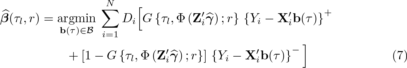
Although they consider more general versions in theoretical parts of their analysis, the practical version of the Arellano and Bonhomme (2017) quantile regression model with selection correction takes the form

Y^{*} = X^{'} β (U)

D = 1 {V \leq p (Z)}

Y = Y^{*} if D = 1

where Y * is the potential outcome, D the selection indicator, and Y the observed outcome (available only for individuals with D = 1). The vectors X and Z are covariate vectors, where X is assumed to be a strict subset of Z (exclusion restriction). The uniformly distributed variable U denotes the rank of the individual in the conditional distribution Y *|X, while the uniformly distributed V represents a normalized error term describing the resistance toward selection. The propensity score p(Z) = P (D = 1|Z) describes the selection probability of individuals with characteristics Z. The propensity score is assumed to follow a probit model; that is, p(Z) = Φ(Z ′γ). The main substantive assumption of the model is that (U, V ) is jointly statistically independent of Z given X.

Equation (1) is a linear quantile regression model for the potential outcome Y * defining the value of Y * that an individual with rank U would get if he or she was selected (for example, the Uth quantile in a distribution of wage offers for individuals with characteristics X). Equation (2) specifies that, among individuals with characteristics Z, a percentage of p(Z) gets selected, but only those whose resistance toward selection V is low enough. Equation (3) states that outcomes are observed only for selected individuals (for example, an individual would earn some wage Y * if he or she decided to work, but this wage is observed only if he or she actually decides to do so)

The interest lies in uncovering the coefficients β(U) characterizing the conditional distribution Y *|X, which includes all individuals with characteristics X, although not all of these individuals actually produce observable outcomes Y . For example, the β(U) describe the pay structure for women with characteristics X, although not all of these women actually take part in the labor market. To establish a link between the quantiles of the distribution of observable outcomes Y and those of the distribution of potential outcomes Y *, Arellano and Bonhomme (2017) observed that

\begin{matrix} P {Y^{*} \leq X' β (τ) | D = 1, Z = z} = P {U \leq τ | V \leq p (z), Z = z} \\ = \frac{C_{U, V | X = x} {τ, p (z)}}{p (z)} : = G_{x} {τ, p (z)} \end{matrix}

where $C_{U, V}_{| X = x} {τ, p (z)} / p (z) = G_{x} {τ, p (z)}$ is the conditional copula of U and V, that is, the probability for an individual with characteristics Z = z to have at most ranks (U, V ) conditional on having at most rank p(z) in the propensity to get selected. Because the left-hand side of (4) describes outcome quantiles in the selected population, this means that the coefficients β(τ) belonging to the τth quantile in the overall population can be recovered by looking at the G _x{τ, p(z)}-quantile observations of the selected population. This establishes the validity of the following “rotated” quantile regression, which uses the observed outcomes Y but applies to them individual specific ranks G _x{τ, p(z)} (instead of the target rank τ).

2.2 Estimation

Based on an independent and identically distributed sample (Y_i, D_i, Z _i ) (with i = 1,…, N and X _i ⊂ Z _i ), Arellano and Bonhomme’s (2017) estimation method proceeds as follows. For practical implementation, one assumes that the true copula C_U,V _| _X=x(u, v) belongs to a parametric family with parameter ρ (such as Gaussian or Frank; see below) and that it does not depend on X. The latter restriction can be relaxed by carrying out estimations by subgroup (see below). The resulting conditional copula function is denoted by G(u, v; ρ). For the following, define a ⁺ = max(a, 0) and a⁻ = max(−a, 0).

Propensity score estimation (step 1)

\hat{γ} = \underset{a \in A}{\arg \min} \sum_{i = 1}^{n} D_{i} In Φ (Z_{i}^{'} a) + (1 - D_{i}) In Φ (- Z_{i}^{'} a)

Estimation of the copula parameter (step 2)

\begin{matrix} \hat{ρ} = \underset{r \in R}{\arg \min} ‖ \sum_{i = 1}^{N} \sum_{l = 1}^{L} (D_{i} φ (Z_{i}) [1 {Y_{i} < X_{i}^{'} \hat{β} (τ_{l}, r)} \\ - G {τ_{l}, Φ (Z_{i}^{'} \hat{γ}); r}]) ‖ \end{matrix}

\begin{matrix} \hat{β} (τ_{l}, r) = \underset{b (τ) \in β}{\arg \min} \sum_{i = 1}^{N} D_{i} [G {τ_{l}, Φ (Z_{i}^{'} \hat{γ}); r} {Y_{i} - X_{i}^{'} b (τ)}^{+} \\ + [1 - G {τ_{l}, Φ (Z_{i}^{'} \hat{γ}); r}] {Y_{i} - X_{i}^{'} b (τ)}^{-}] \end{matrix}

Rotated quantile regression (step 3)

\hat{β} (τ) = \underset{b (τ) \in β}{\arg \min} \sum_{i = 1}^{N} D_{i} [{\hat{G}}_{τ, i} {Y_{i} - X_{i}^{'} b (τ)}^{+} + (1 - {\hat{G}}_{τ, i}) {Y_{i} - X_{i}^{'} b (τ)}^{-}]

Step 1 estimates the probit parameters of the propensity score. Step 2 is a generalized method of moments estimating equation for the copula parameter ρ, which is identified by the conditional moment condition

E [1 {Y_{i} < X_{i}^{'} β (τ)} - G {τ, Φ (Z_{i}^{'} γ); ρ} | D = 1, Z = z] = 0

[following from (4)]. As an instrumental variable for estimating ρ in (6), one can use a suitable function φ(Z _i ) of Z _i , for example, φ(Z _i ) = Φ( $Z_{i}^{'}$ γ). Minimization in (6) is carried out over a grid of candidate values for the copula parameter r ∊ R. For each candidate value r, the estimated $\hat{β}$ (τ_l, r) in (6) are obtained by rotated quantile regression over a grid of auxiliary quantiles τ ₁ ,…, τ_L [see (7)]. Step 3 estimates, for any desired τ, selection-corrected quantile regressions based on the preestimated copula parameter $\hat{ρ}$ . For this, individual-specific rotated ranks ${\hat{G}}_{τ, i}$ = G{τ, Φ( $Z_{i}^{'}$ $\hat{γ}$ ); $\hat{ρ}$ } are used.This can be seen by comparing (8) with the (infeasible) quantile regression, which would be carried out if potential outcomes Y * were observed for the whole population (that is, if there was no selection problem),

\tilde{β} (τ) = \underset{b \in β}{\arg \min} \sum_{i = 1}^{N} D_{i} {{τ (Y_{i}^{*} - X_{i}^{'} b)}^{+} + (1 - τ) {(Y_{i}^{*} - X_{i}^{'} b)}^{-}}

Note that, if one is interested only in β(τ ₁),…, β(τ_L ), step 3 is not necessary, because these are already estimated in step 2. However, for computational reasons and for reasons of flexibility, it may be useful to separate steps 2 and 3. For example, one may already have obtained individual specific copula estimates ${\hat{G}}_{τ, i}$ (for example, by subgroup estimation) and then carried out the desired rotated quantile regressions of step 3 conditional on these preestimated quantities (also see below).

2.3 Inference

Arellano and Bonhomme (2017) showed that the estimators defined in (6), (7), and (8) are asymptotically normal. However, the resulting form of the asymptotic variance matrix is very complex. This makes the use of resampling techniques attractive. In their empirical application, Arellano and Bonhomme (2017) used subsampling (Politis, Romano, and Wolf 1999). An alternative is the bootstrap (for example, Shao and Tu [1995]). The bootstrap draws independent and identically distributed resamples of size N from the original sample and repeats the estimation for several bootstrap replications. The empirical distribution of the bootstrap replications then serves as an estimate of the asymptotic distribution. Subsampling draws subsamples of size m < N without replacement from the original sample and repeats the estimation on the subsamples to obtain an estimate of the asymptotic distribution (after rescaling by m/N). A related method is the m-out-of-n bootstrap, which also draws subsamples of size m < N from the original sample but with replacement. Subsampling and the m-out-of-n bootstrap require that N → ∞ and m/N → 0; that is, the subsamples are required to be small in relation to the sample size N.¹

Subsampling and the m-out-of-n bootstrap work under more general conditions than the bootstrap. In particular, they do not require that the asymptotic distribution be normal. It suffices that a suitably normalized version of the estimator has a limit distribution (Politis, Romano, and Wolf 1999). The bootstrap is guaranteed to work if the limit distribution is normal (Shao and Tu 1995). In the given case, both methods will work because the limit distribution is known to be normal. Subsampling and the m-out-of-n bootstrap are attractive for computational reasons if the sample size is very large because estimations have to be repeated on smaller portions of the data only. However, subsampling and the m-out-of-n bootstrap have to deal with the difficult issue of determining the subsample size (for example, Politis, Romano, and Wolf [1999]; Chernozhukov and Fernández-Val [2005]; Bickel and Sakov [2008]). Based on Chernozhukov and Fernández-Val (2005), Arellano and Bonhomme (2017) used a subsample size of a constant plus the square root of the sample size, where the constant is chosen such that the subsamples are large enough to ensure a reasonable finite sample performance of the estimator (Arellano and Bonhomme 2017, footnote 19).

Our version of Arellano and Bonhomme’s (2017) estimator implements the m-outof-n bootstrap as well as the conventional bootstrap.

2.4 Algorithms

It is well known that quantile regression problems such as (9) can be solved using linear programming techniques. However, the rotated versions (7) and (8) cannot be handled with standard implementations of quantile regression such as qreg, because these do not allow for individual specific ranks ${\hat{G}}_{τ, i}$ . An exception are the codes of Morillo, Koenker, and Eilers (available at http://www.econ.uiuc.edu/∼roger/research/rq/rq.m), also used by Arellano and Bonhomme (2017). For our implementation of Arellano and Bonhomme (2017), we translated these codes from MATLAB to Mata. The codes are based on an interior point algorithm (Koenker 2005) as opposed to the exterior point algorithm used in the current version of qreg. Our experience was that the interior point algorithm converged considerably faster than that used in qreg for most of the datasets analyzed by us. Our implementation also includes safeguards against problems related to using copula values too close to the boundary cases of the counter and the comonotonicity copula (in this case, ${\hat{G}}_{τ, i}$ → 0 or ${\hat{G}}_{τ, i}$ → 1; see the ado-file).

Our implementation allows sampling weights (as used in the empirical application of Arellano and Bonhomme [2018], which we replicate in section 4.2). If sampling weights are specified, we premultiply observations Y_i, X _i , and φ(Z _i ) with the sampling weight of observation i before carrying out all calculations. This ensures that the sums over i = 1,…, N in (6) to (8) are weighted sums. In addition, we include weights in (5).

2.5 Copula functions

Our implementation allows the user to choose among four copula functions, as shown in table 1 (for an overview of copula functions and their properties, see Joe [2015]). An important feature of all of these copulas is that they contain as limit cases the extreme forms of positive (or negative) dependence described by the comonotonicity (countermonotonicity) copula. Not restricting the strength of dependence between U and V (and therefore the strength of selection) appears to be important to avoid imposing restrictions that are not compatible with the data. Out of the four copulas listed in table 1, the Frank, Gaussian, and Plackett copulas can represent only symmetrical patterns, while the Joe and Ma (2000) copula can also accommodate asymmetrical patterns (Joe 2015).

Table 1.

Copula functions C(u, v; ρ)

Frank copula

- \frac{1}{ρ} \log {1 + \frac{(e^{- ρ u} - 1) (e^{- ρ v} - 1)}{e^{- ρ} - 1}} \forall ρ \in ℝ

Gaussian copula

Φ_{2} {Φ^{- 1} (u), Φ^{- 1} (v); ρ} \forall ρ \in (- 1, 1)

Plackett copula

\begin{array}{l} \frac{1}{2 (ρ - 1)} (1 + (ρ - 1) (u + v) - [{1 + (ρ - 1) (u + v)}^{2} \\ - 4 (ρ - 1) u v]^{\frac{1}{2}}) \forall ρ \in (0, \infty) \end{array}

Joe and Ma (2000) copula

1 - F_{r} ({[{F_{Γ}^{- 1} (1 - u; ρ)}^{ρ} + {F_{Γ}^{- 1} (1 - v; ρ)}^{ρ}]}^{\frac{1}{ρ}}) \forall ρ \in (0, \infty)

SOURCE: Joe (2015). F _Γ(·, a) is the cumulative Gamma distribution with shape parameter a.

Because the value of the copula parameter ρ typically has no direct interpretation, our estimation command reports standard measures of bivariate concordance as listed in table 2. These represent generalized measures of correlation between U and V, which are a function of the copula and the copula parameter (Joe 2015). The concordance measures describe the association between the rank in the latent outcome distribution U and that in the distribution of resistance toward selection V . For example, if high values of U are associated with low values of V, then individuals who get selected tend to have higher outcomes than those who do not (positive selection). Note that positive (or negative) selection will be represented by negative (or positive) concordance measures because of the definition of V as the resistance toward selection.

Table 2.

Bivariate concordance measures

Spearman’s rank correlation

ρ s = 12 \int_{0}^{1} \int_{0}^{1} u v d C (u, v; ρ) - 3

Kendall’s tau

\begin{array}{l} τ_{K} = P {(U_{1} - U_{1}^{'}) (V_{2} - V_{2}^{'}) > 0} - P {(U_{1} - U_{1}^{'}) (V_{2} - V_{2}^{'}) < 0} \\ = \int_{0}^{1} \int_{0}^{1} C (u, v; ρ) d C (u, v; ρ) \end{array}

Blomqvist’s beta

\begin{array}{l} β_{b 1} = P {(U - \frac{1}{2}) (V - \frac{1}{2}) > 0} - P {(U - \frac{1}{2}) (V - \frac{1}{2}) < 0} \\ = 4 C (\frac{1}{2}, \frac{1}{2}; ρ) - 1 \end{array}

SOURCE: Joe (2015).

The interpretation of the different concordance measures is as follows. Spearman’s rank correlation measures the (ordinary) correlation between the ranks U and V . Kendall’s tau is positive if it is more likely that ranks go into the same rather than into opposite directions, and it is negative otherwise. Blomqvist’s beta is positive if it is more likely that both ranks U and V lie on the same side of the median rank (which is one half) than on opposite sides.

3 The arhomme command

3.1 Syntax

arhomme depvar [ indepvars ] [ if ] [ in ] [ weight ] ,

select( [ depvar_s ] [ = ] varlist_s ) [ rhopoints(#) taupoints(#) meshsize(#) centergrid(#) frank gaussian plackett joema nostderrors subsample(#) repetitions(#) fillfraction(#) instrument(varname) copulaparameter(varname) quantiles(# [ # [ # … ] ]) graph output( [ normal ] [ bootstrap ] ) ]

pweights are allowed; see [U] 11.1.6 weight.

arhomme is byable.

3.2 Options

3.2.1 Selection

select( [ depvar_s ] [ = ] varlist_s ) specifies the variables and options for the selection equation. It is an integral part of specifying the Arellano and Bonhomme (2017) model and is required. The selection equation must contain at least one variable that is not in the outcome equation.

If depvar_s is specified, it should be coded as 0 or 1, with 0 indicating an observation not selected and 1 indicating a selected observation. If depvar_s is not specified, observations for which depvar is not missing are assumed selected and those for which depvar is missing are assumed not selected.

3.2.2 Grid tuning

rhopoints(#) determines the number of candidate points for the copula parameter grid search. The default is rhopoints(19). When the option frank is chosen, the copula candidate values are constructed as follows. First, the unit interval is divided into (# + 1) equidistant intervals. Then, the ith candidate is defined as the ith quantile of a Cauchy distribution with scale meshsize() and shift centergrid(). With the option gaussian, the quantiles of a sinus density with emphasis centergrid() and range meshsize()× (1 − |centergrid()|) are built. The grid for the copula options plackett and joema is designed as the square root of the ith unit interval point divided by 1 minus this point. This method ensures that the resulting grid is denser around centergrid(). The user can shift the focus of the grid search by specifying the desired centergrid(), by reducing (or increasing) meshsize(), or by increasing (or reducing) rhopoints(). Note that the default rhopoints(19) is likely to be too small for many applications.

taupoints(#) specifies the number of quantiles for which the moment restriction is supposed to hold (step 2 in Arellano and Bonhomme [2017]). We recommend using this option with graph. The resulting scatterplot should suggest a smooth objective function (at least around the gravity center of search; the objective function may look erratic toward outer values no matter how many taupoints() are used). Increase taupoints() to further smooth the objective function. The default taupoints(3) is a good start in many applications, but many taupoints() are recommended for more reliable estimates.

meshsize(#) scales the grid search interval up (or down). For large #, the resulting grid becomes less dense but searches a wider range. # is restricted to strictly positive real values for the options frank, plackett, and joema and is restricted to (0, 1] when using gaussian. The default meshsize(1) tends to be a good start.

centergrid(#) sets the gravity center of the grid. If you already suspect the optimal copula parameter to be a specific value, this option helps shift the emphasis of your search. # is restricted to (−1, 1) with gaussian and to (0, ∞) for plackett and joema, and it is unrestricted with frank. By default, the grid will always be symmetric about the independence copula, that is, centergrid(0) for frank and gaussian, and centergrid(1) for plackett and joema.

frank specifies the Frank copula to model individually rotated quantiles. The copula parameter is ρ ∊ ℝ, with ρ → −∞ corresponding to the lower Fréchet–Hoeffding bound, ρ = 0 to the independence copula, and ρ → ∞ to the upper Fréchet–Hoeffding bound.

gaussian specifies the Gaussian copula used to model individually rotated quantiles. The copula parameter is ρ ∊ (−1, 1), with ρ → −1 corresponding to the lower Fréchet–Hoeffding bound, ρ = 0 to the independence copula, and ρ → 1 to the upper Fréchet–Hoeffding bound.

plackett specifies the Plackett copula used to model individually rotated quantiles. The copula parameter is ρ ∊ (0, ∞), with ρ → 0 corresponding to the lower Fréchet– Hoeffding bound, ρ = 1 to the independence copula, and ρ → ∞ to the upper Fréchet–Hoeffding bound. If standard errors are computed, the copula parameter is tested for ρ = 1 instead of ρ = 0. The p-value is reported accordingly.

joema specifies the Joe and Ma (2000) copula to model individually rotated quantiles. The copula parameter is ρ ∊ (0, ∞), with ρ → 0 corresponding to the lower Fréchet– Hoeffding bound, ρ = 1 to the independence copula, and ρ → ∞ to the upper Fréchet–Hoeffding bound. If standard errors are computed, the copula parameter is tested for ρ = 1 instead of ρ = 0. The p-value is reported accordingly.

3.2.3 Standard errors/subsampling

nostderrors disables the computation of standard errors. This option precludes the use of subsample(#) and repetitions(#).

subsample(#) draws samples of size # with replacement from the marked dataset. Standard errors are computed by the m-out-of-n bootstrap method. If # is greater than or equal to the effective size of the entire dataset, the conventional bootstrap is executed.

repetitions(#) specifies the number of bootstrap replications to be used to obtain an estimate of the variance–covariance matrix of the estimators. The default is repetitions(100), which is likely to be too small in many applications.

fillfraction(#) determines up to which fraction of overall bootstrap repetitions the program replaces subsamples in case of failed convergence. If this limit is reached, further failed subsamples are dropped without being replaced. The default is fillfraction(.3).

3.2.4 Instrument/copula parameter

instrument(varname) lets the user define a variable in the dataset that serves as the instrument to estimate the copula parameter [see (6)]. The instrument has to be a function of varlist_s . The default is the propensity score.

copulaparameter(varname) indicates that the copula parameter has already been estimated by the user (for example, separately by sample subgroups in a first stage) and stored per observation in the variable varname. In this case, only step 3 of Arellano and Bonhomme (2017) is performed (estimation of the selection-corrected quantile coefficients). The values in varname are restricted to (−1, 1) with the option gaussian and to the positive real line for plackett and joema. They are unrestricted for frank. This option must be used in connection with nostderrors and precludes the use of rhopoints(), taupoints(), meshsize(), centergrid(), subsample(), repetitions(), instrument(), and graph. The reason is that the user will have to code his or her own bootstrap procedure, including all the different stages of his or her estimations (for example, using bootstrap). It is only in this way that the sampling variability of the preestimated copula parameters is accounted for.

3.2.5 Reporting

quantiles(# [ # [ # … ] ]) specifies the quantiles to be estimated. Valid inputs range from 0 to 1, exclusively, and in ascending order. The default is quantiles(0.1(0.1)0.9) corresponding to all deciles.

graph specifies that a scatterplot of all objective function values be automatically generated after estimation.

output( [ normal ] [ bootstrap ] ) defines whether the output table generated is based on the asymptotic, that is, normal, or the bootstrap distribution. If both are specified, two separate output tables are produced. The first stage (probit) standard errors in the output are always asymptotic (coming from the default probit command). repetitions() should always be set to at least 500 when choosing output(bootstrap). If both normal and bootstrap are specified, then results based on the normal distribution are reported first.

4 Empirical examples

4.1 Comparison with Heckman selection model

Our first empirical illustration uses the example in the Stata manual for the command heckman, which fits the Heckman (1979) selection model for the mean outcome.

The result of using heckman is

We then use arhomme to fit a selectivity-corrected regression model for the median. For doing this, we also illustrate a useful stepwise procedure to arrive at a reasonable choice for the grid used to estimate the copula parameter.

A first step is

We then use a refined grid:

So far, we have used the option nostd to save computing time. In the next step, we also include the computation of standard errors:

Both heckman and arhomme find substantial positive selection (recall that a negative copula parameter in arhomme represents positive selection). The coefficients for education and age in arhomme for the median wage are quite similar to those for the mean wage in heckman. This will be the likely outcome if the conditional distributions are symmetric (implying that the mean is equal to the median).

Finally, we illustrate the postestimation features of arhomme:

4.2 Replication of Arellano and Bonhomme (2018)

This section replicates the empirical example in Arellano and Bonhomme (2018). The data are from Huber and Melly (2015) and can be downloaded from the Journal of Applied Econometrics data archive (http://qed.econ.queensu.ca/jae/2015-v30.7/hubermelly/). The application refers to the returns to education and experience for women in the United States using data from the 2011 Current Population Survey. The sample covers white non-Hispanic women aged between 25 and 54 years. Individuals who are self-employed or work for the military, public, or agricultural sector are excluded. Working is defined as having worked for more than 35 hours in the week preceding the survey. The application uses the Current Population Survey sampling weights.

We first load the data and modify some of the variable names to make them conform to those used in Arellano and Bonhomme (2018):

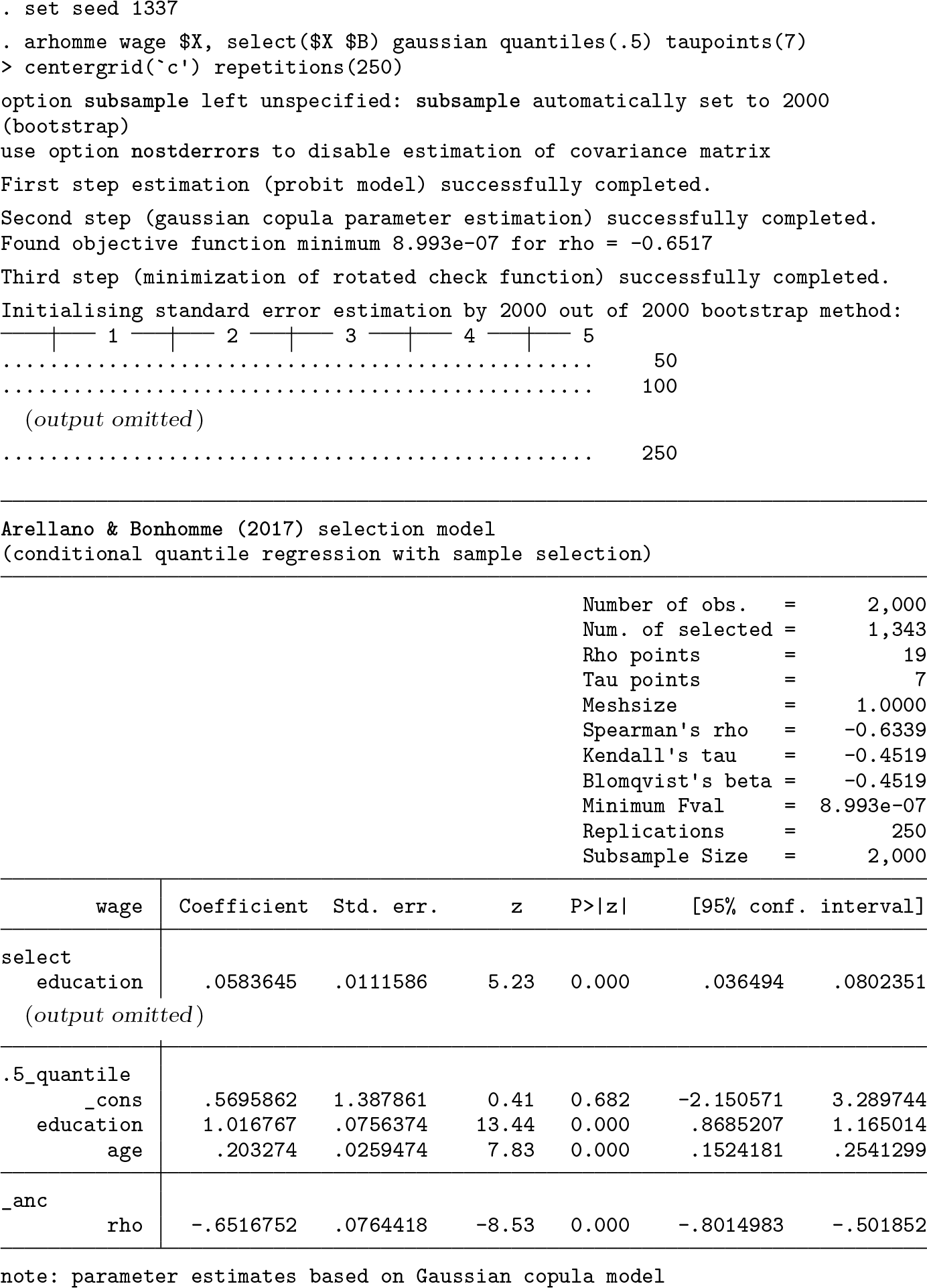
We now apply arhomme, following as closely as possible the specification in Arellano and Bonhomme (2018):

The results for the selection-corrected quantile regression coefficients are almost identical to those reported by Arellano and Bonhomme (2018, table 1). Standard-error estimates are also very similar. The point estimate for the copula parameter and its standard error also come close to those reported by Arellano and Bonhomme (2018) ( $\hat{ρ}$ = −0.10 with standard error 0.054). Small differences between our results and those of Arellano and Bonhomme (2018) are to be expected because standard errors are the result of a random process (subsampling), because of numerical software differences, and because we do not know the exact choices of Arellano and Bonhomme (2018) for grid search, number of supporting quantiles, etc.

4.3 Partial replication of Arellano and Bonhomme (2017)

Our last empirical example replicates selected results in Arellano and Bonhomme (2017). wagedata.dta can be downloaded from Stéphane Bonhomme’s webpage (https://sites. google.com/site/stephanebonhommeresearch/) and refers to selectivity-corrected wage distributions for the UK for the period 1978–2000. This section illustrates the use of the graph option, which displays the grid search optimization for the copula parameter.

To replicate a selected quantile regression for the subgroup of single females, we first run some preparatory steps (taken from the file sample_construction.do, which can also be downloaded from the above webpage; details are available on request).

We then start with a first crude estimation attempt:

Figure 1.

Plot of objective function over crude grid

Refine grid:

Figure 2.

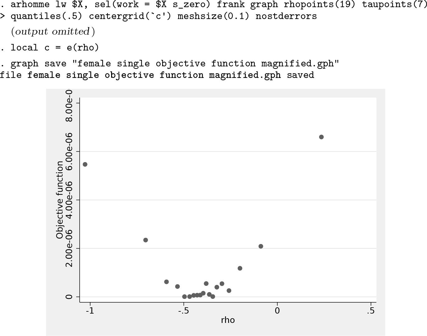
Plot of objective function over refined grid

Finally, we estimate the preferred specification with standard errors based on subsampling (using the same subsample size as in Arellano and Bonhomme [2017]):

Arellano and Bonhomme (2017) do not document their estimated selectivity-corrected regression coefficients (they are used only in their later calculations), but they do report estimated copula parameters for different population subgroups. For the group of single females, they report an estimated Spearman rank correlation of −0.080 (Arellano and Bonhomme 2017, 16) and an estimated parameter for the Frank copula of −0.4820 (documented in replication file Graphs_Frank_copula.m downloadable from Stéphane Bonhomme’s webpage; see above). Up to numerical differences, this is very close to the results we obtain above.

5 Conclusion

In this article, we described a command, arhomme, implementing the Arellano and Bonhomme (2017) method of sample selection correction for quantile regressions along with standard errors based on bootstrapping and subsampling. arhomme is fast and potentially applicable in many fields in which there is a need to correct estimates of conditional distributions for sample selection. If one is interested in obtaining unconditional distributions corrected for sample selection, the resulting conditional distributions may be aggregated up as described in Albrecht, van Vuuren, and Vroman (2009) or Chernozhukov, Fernández-Val, and Melly (2013).

Supplemental Material

Supplemental Material, sj-zip-1-stj-10.1177_1536867X211045516 - arhomme: An implementation of the Arellano and Bonhomme (2017) estimator for quantile regression with selection correction

Supplemental Material, sj-zip-1-stj-10.1177_1536867X211045516 for arhomme: An implementation of the Arellano and Bonhomme (2017) estimator for quantile regression with selection correction by Martin Biewen and Pascal Erhardt in The Stata Journal

Footnotes

6 Acknowledgments

We thank Michael Wolf (University of Zürich) for discussions and advice on subsampling. We also thank Ben Jann, Blaise Melly, Philippe Van Kerm, and the participants of the Swiss Stata Conference 2020 for many helpful comments and suggestions. Financial support through the DFG Priority Program 1764 and DFG project BI 767/3-1 is gratefully acknowledged.

7 Programs and supplemental materials

To install a snapshot of the corresponding software files as they existed at the time of publication of this article, type

Notes

References

Ahn

Powell

J. L.

1993. Semiparametric estimation of censored selection models with a nonparametric selection mechanism. Journal of Econometrics 58: 3–29. https://doi.org/10.1016/0304-4076(93)90111-H.

Albrecht

van Vuuren

Vroman

2009. Counterfactual distributions with sample selection adjustments: Econometric theory and an application to the Netherlands. Labour Economics 16: 383–396. https://doi.org/10.1016/j.labeco.2009.01.002.

Andrews

D. W. K.

Schafgans

M. M. A.

1998. Semiparametric estimation of the intercept of a sample selection model. Review of Economic Studies 65: 497–517. https://doi.org/10.1111/1467-937X.00055.

Arellano

Bonhomme

2017. Quantile selection models with an application to understanding changes in wage inequality. Econometrica 85: 1–28. https://doi.org/10.3982/ECTA14030.

Arellano

Bonhomme

2018. Sample selection in quantile regression: A survey. In Handbook of Quantile Regression, ed. Koenker

Chernozhukov

Peng

, chap. 13. Handbooks of Modern Statistical Methods, Boca Raton, FL: Chapman & Hall/CRC. https://doi.org/10.1201/9781315120256-13.

Bickel

P. J.

Sakov

2008. On the choice of m in the m out of n bootstrap and confidence bounds for extrema. Statistica Sinica 18: 967–985.

Biewen

Fitzenberger

Seckler

2020. Counterfactual quantile decompositions with selection correction taking into account Huber/Melly (2015): An application to the German gender wage gap. Labour Economics 67: 101927. https://doi.org/10.1016/j.labeco.2020.101927.

Bollinger

C. R.

Hirsch

B. T.

Hokayem

C. M.

Ziliak

J. P.

2019. Trouble in the tails? What we know about earnings nonresponse 30 years after Lillard, Smith, and Welch. Journal of Political Economy 127: 2143–2185. https://doi.org/10.1086/701807.

Buchinsky

1998. The dynamics of changes in the female wage distribution in the USA: A quantile regression approach. Journal of Applied Econometrics 13: 1–30. https://doi.org/10.1002/(SICI)1099-1255(199801/02)13:1<1::AID-JAE474>3.0.CO;2-A.

10.

Buchinsky

2001. Quantile regression with sample selection: Estimating women’s return to education in the U.S. Empirical Economics 26: 87–113. https://doi.org/10.1007/s001810000061.

11.

Chen

Khan

2003. Semiparametric estimation of a heteroskedastic sample selection model. Econometric Theory 19: 1040–1064. https://doi.org/10.1017/S0266466603196077.

12.

Chernozhukov

Fernández-Val

2005. Subsampling inference on quantile regression processes. Sankhyā 67: 253–276.

13.

Chernozhukov

Fernández-Val

Melly

2013. Inference on counterfactual distributions. Econometrica 81: 2205–2268. https://doi.org/10.3982/ECTA10582.

14.

Das

Newey

W. K.

Vella

2003. Nonparametric estimation of sample selection models. Review of Economic Studies 70: 33–58. https://doi.org/10.1111/1467-937X.00236.

15.

D’Haultfoeuille

Maurel

Qiu

Zhang

2020. Estimating selection models without an instrument with Stata. Stata Journal 20: 297–308. https://doi.org/10.1177/1536867X20930998.

16.

Fernández-Val

van Vuuren

Vella

2018. Nonseparable sample selection models with censored selection rules: An application to wage decompositions. IZA Discussion Paper No. 11294, Institute of Labor Economics (IZA). http://ftp.iza.org/dp11294.pdf.

17.

Gronau

1974. Wage comparisons–A selectivity bias. Journal of Political Economy 82: 1119–1143. https://doi.org/10.1086/260267.

18.

Heckman

J. J.

1974. Shadow prices, market wages, and labor supply. Econometrica 42: 679–694. https://doi.org/10.2307/1913937.

19.

Heckman

J. J.

1979. Sample selection bias as a specification error. Econometrica 47: 153–161. https://doi.org/10.2307/1912352.

20.

Huber

Melly

2015. A test of the conditional independence assumption in sample selection models. Journal of Applied Econometrics 30: 1144–1168. https://doi.org/10.1002/jae.2431.

21.

Joe

2015. Dependence Modeling with Copulas. Boca Raton, FL: CRC Press.

22.

Joe

2000. Multivariate survival functions with a min-stable property.Journal of Multivariate Analysis 75: 13–35. https://doi.org/10.1006/jmva.1999.1891.

23.

Koenker

2005. Quantile Regression. New York: Cambridge University Press.

24.

Maasoumi

Wang

2019. The gender gap between earnings distributions. Journal of Political Economy 127: 2438–2504. https://doi.org/10.1086/701788.

25.

Picchio

Mussida

2011. Gender wage gap: A semi-parametric approach with sample selection correction. Labour Economics 18: 564–578. https://doi.org/10.1016/j.labeco.2011.05.003.

26.

Politis

D. N.

Romano

J. P.

Wolf

1999. Subsampling. New York: Springer.

27.

Shao

1995. The Jackknife and Bootstrap. New York: Springer.

Supplementary Material

Please find the following supplemental material available below.

For Open Access articles published under a Creative Commons License, all supplemental material carries the same license as the article it is associated with.

For non-Open Access articles published, all supplemental material carries a non-exclusive license, and permission requests for re-use of supplemental material or any part of supplemental material shall be sent directly to the copyright owner as specified in the copyright notice associated with the article.

0.00 MB