Sage Journals: Discover world-class research

Abstract

In this article, we present a new command, qcte, that implements several methods for estimation and inference for quantile treatment-effects models with a continuous treatment. We propose a semiparametric two-step estimator, where the first step is based on a flexible Box–Cox model, as the default model of the command. We develop practical statistical inference procedures using bootstrap. We implement some simulations to show that the proposed methods perform well. Finally, we apply qcte to a survey of Massachusetts lottery winners to estimate the unconditional quantile effects of the prize amount, as a proxy of nonlabor income changes, on subsequent labor earnings from U.S. Social Security records. The empirical results reveal strong heterogeneity across unconditional quantiles.

Keywords

st0597 qcte continuous treatment quantile treatment effects quantile regression

1 Introduction

The effect of policy variables on distributional outcomes are of fundamental interest in empirical economics and of importance for policymakers. The treatment-effects (TE) literature has been extensively used in economics to analyze how treatments or social programs affect selected outcomes of interest. On the binary TE models, Hahn (1998); Heckman et al. (1998); Hirano, Imbens, and Ridder (2003); Abadie and Imbens (2006); and Li, Racine, and Wooldridge (2009) study efficient estimation of the average TE. The Stata teffects command can be used to implement these. There is also a lot of literature on exploring effects of heterogeneity using unconditional quantiles, quantile TE. See, for example, Chernozhukov and Hansen (2005) and Firpo (2007). Many of these can be implemented following Frölich and Melly’s (2010) package, ivqte. See also Hasebe (2013) for an alternative estimator.

There is also literature on estimation of multivalued TE, which can be implemented with the package poparms; see, for example, Imbens (2000); Lechner (2001); Cattaneo (2010); and Cattaneo, Drukker, and Holland (2013). It is known, however, that categorizing or discretizing continuous treatments generally leads to several serious problems, such as loss of power in testing, misclassification (which is associated with potential bias), problems with prediction, and even problems with interpretation of the results and coefficients of interest. See, for example, Cox (1957); Cohen (1983); van Belle (2008); and Fedorov, Mannino, and Zhang (2009) for more comprehensive discussions on problems associated with discretizing continuous variables. Recently, there has been a growing interest in continuous TE. Continuous treatments (such as those indexed by dose, exposure, duration, or frequency) arise often in practice, especially in observational studies. More importantly, such treatments lead to effects that are naturally described by curves (for example, dose–response curves as functionals of the treatment dose) rather than scalars (for example, point estimators) as in discrete treatments. Many articles in the literature on unconditional TE concentrate on discrete treatments, that is, binary or multivalued treatment assignments. Among others, Hirano and Imbens (2004) and Imai and van Dyk (2004) develop a generalized propensity score for continuous average treatment models to estimate average dose–response functions (ADRF) and average continuous TE (ACTE). Other estimators were proposed by Flores (2007) and Flores et al. (2012). Bia and Mattei (2008) and Bia et al. (2014) propose two commands, gpscore and drf, that compute the ADRF and ACTE using parametric and semiparametric techniques.

Galvao and Wang (2015) and Alejo, Galvao, and Montes-Rojas (2018) derive a twostep estimator for practical estimation and inference for quantile TE with continuous treatment. A parameter of interest in the presence of continuous treatment is the entire curve of quantile potential outcomes or quantile dose–response functions (QDRF). The QDRF summarizes the potential responses of each dose of magnitude t ∊ [texmath]T[/texmath] on a specified outcome of interest at the unconditional quantile τ ∊ (0, 1). Another parameter of interest is the quantile continuous treatment effect (QCTE), which corresponds, for any fixed quantile, to the difference between two QDRF at given levels of treatment. Identification of the parameters of interest is based on the ignorability or weak unconfoundedness assumption (see, for example, Rubin [1977], Heckman et al. [1998], or Dehejia and Wahba [1999]), applying the methodology of Galvao and Wang (2015). The estimators are implemented as two-step estimators. In the first step, one estimates a ratio of conditional densities. In the second step, one performs a simple weighted quantile regression estimation where the weights are given by the ratio of conditional density functions. Alejo, Galvao, and Montes-Rojas (2018) propose a flexible Box–Cox density estimation procedure. This approach has important advantages. The first advantage is that the first step of the Box–Cox procedure is simple to implement in practice. The second advantage is that the Box–Cox procedure allows for many covariates and satisfies the required convergence rates for the first step. The Box–Cox procedure is thus flexible to accommodate empirical settings where the ignorability assumption is valid only after conditioning on a rich (possibly large) set of covariates. The numerical simulations show that the Box–Cox procedure is a flexible procedure that correctly estimates QDRF and QCTE functions for alternative data-generating processes.

In this article, we present a new command, qcte, that estimates both QDRF and QCTE. Unconditional quantile heterogeneity thus complements the results of ADRF and ACTE.

We evaluate the finite-sample performance of the proposed estimator in two ways. First, we implement Monte Carlo simulation exercises. In particular, we evaluate location shift and scale-location shift data-generating processes. Second, to illustrate the methods, we estimate the effects of nonlabor income changes on labor earnings. We use the survey of Massachusetts lottery winners and estimate the effect of the prize amount, as a proxy of exogenous nonlabor income changes, on subsequent labor earnings (from U.S. Social Security records). This database was originally used by Imbens, Rubin, and Sacerdote (2001) and then by Hirano and Imbens (2004). The lottery prize, being unrelated with labor market performance, conditional on a rich set of observables, serves as an income shock that may be used to measure the income effect on labor market decisions. In this example, we have interest in identifying the effect of the lottery prize, which is a continuous variable, on labor earnings, and as such in estimating the QDRF and QCTE curves. That is, rather than studying the effect on a treatment group (that is, with income shock) with respect to a comparable control group, we are interested in the curve linking labor market variables with the size of the shock. We focus on yearly income size years after the prize was received. The quantile process shows important heterogeneity in the marginal effects of the lottery prize. In particular, higher quantiles of future labor market earnings are less responsive to an increment in the lottery prize than lower quantiles. These results are important for analyzing the effect of general income transfers as conditional cash transfer programs in developing countries because the quantile heterogeneity reveals that those that are more likely to opt out of the labor market are the ones in the lower part of the income distribution.

The remainder of the article is organized as follows. In section 2, we review the QCTE estimator of Alejo, Galvao, and Montes-Rojas (2018). In section 3, we describe the qcte syntax. In section 4, we illustrate the procedure by applying the command to Monte Carlo simulation and to the empirical application of the survey of Massachusetts lottery winners used by Hirano and Imbens (2004). In section 5, we conclude with practical suggestions on the proper use of the command.

2 Continuous treatment effects

We want to learn how an outcome variable changes as the dose of some treatment variable varies. The dose is denoted by t, where $t \in T$ , an interval in $ℝ$ , and the outcome is denoted by Y (t). More specifically, for each $t \in T$ , Y (t) is the outcome when the dose of treatment is t. Thus, define the random process Y (t) as t varies in T. In the binary treatment case, $T = {0, 1}$ . For practical convenience, we assume T to be an interval [t ₀ , t ₁], and therefore the dose values of interest will be on that compact set.

An important parameter of interest when the treatment is continuous is the QDRF, which is defined as

q_{τ} (t) \in i n f {q : F_{Y (t)} (q) \geq τ} τ \in (0, 1)

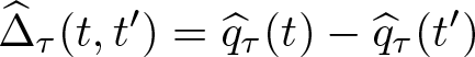
the unconditional τth QDRF, where F_Y _(t) is the distribution function of Y (t). Thus, the QDRF summarizes the potential responses of each dose of magnitude $t \in T$ on a specified outcome of interest, Y (t), at its unconditional quantile τ.

From the QDRF, one can learn about another interesting parameter, the QCTE, which is defined as

Δ_{τ} (t, t') : = q_{τ} (t) - q_{τ} (t')

for t′ < t. The QCTE, as defined in (1), captures the difference of the τth quantile at two given different levels of treatment, t and t′. This QCTE function is the same as defined in Lee (2018) and describes the difference between the two potential responses of Y (t) at doses of magnitude t and t′, at a given unconditional quantile τ. Note that in this article, the QCTE is defined as the difference of the τth quantile at different levels of treatment. This definition does not require the assumption of rank preservation, and it is regarded as a convenient way to summarize interesting aspects of marginal distributions of the potential outcomes. However, if rank preservation holds, then the QCTE defined above has a causal interpretation, that is, the effect of changing the level of the treatment for any particular subpopulation. See Firpo (2007) and Cattaneo (2010) for detailed discussions on rank preservation in quantile TE and definitions of concepts. Of particular interest is analyzing the QCTE for a fixed change in the dose, say, δ > 0, over the doses $t \in T$ as

D_{τ} (t, δ) : = Δ_{τ} (t + δ, t) = q_{τ} (t + δ) - q_{τ} (t)

Unfortunately, as is usual in the TE literature, one cannot observe Y (t) for all $t \in T$ . Rather, only a single Y (t ₀) can be observed, where t ₀ is the realization of a random variable T . Hence, if assignment to treatment status depends on potential outcomes, as is usual in economic and other nonexperimental problems, then selection biases arise because the observed outcomes might not be the result of the dose itself but of self-assignment into treatment. To solve this problem, it is common in the TE literature to assume the existence of a set of random variables X , conditional on which Y (t) is independent from T for all $t \in T$ . Thus, conditional on observable variables, observed outcomes can be given a causal interpretation. This is the ignorability condition or weak unconfoundedness assumption in the literature. Finally, we need to combine the results for X to obtain an unconditional TE. By the law of iterated expectations, unconditional expectations can be recovered.

Define m{Y (t); q_τ (t)} = τ − 1{Y (t) < q_τ (t)} for each t and let

E [m {Y (t); q_{τ} (t)}] = 0

Thus, q_τ (t) is defined as the solution to the moment condition given by (3). If this problem has a unique solution, the identification result relies on the following equality,

E [m {Y (t); q_{τ} (t)}] = E [m {Y; q_{τ} (t)} w_{0} (U; t)]

for each $t \in T$ , where w ₀( u ; t) := {f_T _{|
X

,Y} (t| x , y)}/{f_T _{|
X}(t| x )}, and for notational convenience, we denote u := ( x ^⊤ , y)^⊤ and U := ( X ^⊤ , Y )^⊤. Consequently,

E [m {Y; q_{τ} (t)} w_{0} (U; t)] = 0

if and only if q_τ (t) = q_τ ₀(t).

This result is a direct application of theorem 1 in Galvao and Wang (2015), who extended the propensity-score method to general dose–response functions in a setting with continuous treatment. The intuition behind the result is that Y (t) being unobserved is replaced with observables ( X , Y, T ) equipped with a proper estimation of the density function of the treatment conditional on ( X , Y ).

As in the TE literature, the identification induces an estimating equation with two pieces, the function m(·) with a weighting function w ₀(·). In our case, the weights are given by {f_T _{|
X

,Y} (t| x , y)}/{f_T _{|
X}(t| x )}. The intuition of this result is similar to the discrete case, where the propensity score is replaced by the corresponding density function. Also note that the weights could be written as {f_Y _{|
X

,T} (y| x , t)}/{f_Y _{|
X}(y| x )}. In either case, we need to work with a ratio of two conditional densities. Note that this approach seems different from Hirano and Imbens (2004) and other articles that followed, where they estimate only f_Y _{|
X}(y| x ), the so-called generalized propensity score. However, Hirano and Imbens’s approach also requires one to estimate E[Y |X, T ], or in fact, E[Y |f_T _|X(t|x), T ]. Thus, Hirano and Imbens’s procedure and ours involve two different functional estimates to compute the parameter of interest.

Finally, because the QCTE is the difference between the QDRF at two different treatment doses, identification of QCTE, Δ _τ (t, t′), is as straightforward as the previous result.

2.1 Two-step estimator

Using the identification expression (4), Alejo, Galvao, and Montes-Rojas (2018) propose a two-step estimator for both QDRF and QCTE, in (1) and (2), respectively, as in Firpo (2007), Cattaneo (2010), and Galvao and Wang (2015). In the first step, one estimates the weights, that is, the ratio of densities, w( u ; t) := {f_T _{|
X

,Y} (t| x , y)}/{f_T _{|
X}(t| x )}. The second step is given by a reweighted version of the standard quantile estimation procedure (Koenker and Bassett 1978). Below, we describe the details of estimation.

We have a random sample of units ( X _i, Y_i, T_i ), indexed by i = 1,…, n. For each unit i, X _i is a vector of covariates, and the level of the treatment received is T_i ∊ [t ₀ , t ₁]. We observe the vector X _i , the treatment received T_i , and the observed outcome corresponding to the level of the treatment received, Y_i .

First step: Estimation of w ₀

To implement the estimator, we need an estimator for w ₀. In practice, one estimates f_T _{|
X

,y}(t| x , y) and f_T _|
X(t| x ) separately and then computes the ratio to estimate w ₀. Galvao and Wang (2015) suggest a potential nonparametric estimation for the first step. However, there are important issues with its practical implementation. The most important is that in several empirical applications, the number of variables in X is relatively large, and because it is well known in the literature, it has an adverse effect on nonparametric methods because of the curse of dimensionality. Therefore, there are compelling reasons to use flexible parametric models to estimate the ratio of the conditional density functions. Following the results of Carroll and Ruppert (1984), Alejo, Galvao, and Montes-Rojas (2018) suggest a flexible Box–Cox estimation. This approach has important advantages. The first advantage is that the first step of the Box–Cox procedure is quick and simple to implement in practice. The second advantage is that the Box–Cox procedure allows for many covariates and satisfies the required convergence rates for the first step.

To estimate the conditional density f_T _{|
X

,Y} (t| x , y), we use the model

Λ (T, λ_{1}) = Λ {(X), λ_{2}} β_{X} + Λ (Y, λ_{2}) β_{Y} + ϵ

where $ϵ | X, Y \sim N (0, σ_{ϵ}^{2})$ and Λ(·, λ) is the Box–Cox transformation function, which is defined as Λ(Z, λ) = log Z if λ = 0 and = (Z^λ − 1)/λ otherwise. Using maximum likelihood estimation, we obtain the unknown set of parameters $µ : = (λ_{1}, λ_{2}, β_{X}, β_{Y}, σ_{ϵ}^{2})$ and finally the conditional density ${\hat{f}}_{T}_{| X, Y} (t | x, y)$ (see appendix A.1 for more details on density formulas). Moreover, we obtain ${\hat{f}}_{T}_{| X} (t | x)$ similarly using the Box–Cox model

Λ (T, λ_{1}) = Λ {(X), λ_{2}} β_{X} + ϵ

The Box–Cox transformation applies only to variables in a positive domain (excluding zero). Nevertheless, this could be implemented if we define, for a given variable x, x ^∗ = e^x , where we could thus have negative, zero, and positive values of x, and we allow the Box–Cox parameters to transform x ^∗. In this case, if the estimated parameter λ is indeed zero, then the variable would require no transformation. Note that the normality assumption is a simplifying condition. The Monte Carlo simulations in Alejo, Galvao, and Montes-Rojas (2018) show that the Box–Cox Gaussian model performs well for a large family of distributions.

As noted by an anonymous referee, the QDRF and QCTE models rely on the assumption that the true conditional density f_T _{|
X

,Y} (t| x , y) or f_T _|
X(t| x ) can be consistently estimated with the Box–Cox procedure. Because we do not know the structure of the conditional models, goodness-of-fit procedures can be used to evaluate the adequacy of the proposed models. In particular, because the Box–Cox estimator is maximum likelihood, the likelihood-ratio test or Akaike and Bayesian criteria can be used to select the best model.

Second step: Estimation of q_τ ₀ and Δ _τ ₀

Following (3), the identification condition for q_τ ₀(t) is E ([τ − 1{Y < q_τ ₀(t)}]w ₀( U ; t)) = 0. Thus, an estimator for the QDRF q_τ ₀(t) is

{\hat{q}}_{τ} (t) = \arg \min_{q} \frac{1}{n} \sum_{i = 1}^{n} \hat{w} (u_{i}; t) ρ_{τ} (y_{i} - q)

where ρ_τ (·) := ·(τ − 1{· < 0}) is the check function as in Koenker and Bassett (1978). Practical implementation of the estimator is simple. In practice, given the random sample ( X , T, Y ), one first computes $\hat{w}$ in the first step as described previously. Then, in the second step, one computes a simple weighted quantile regression of Y on a constant term using $\hat{w}$ as weights as given in (5), for each given t taken over a discretized subset (that is, grid) of T.

Estimation of the QCTE parameter, Δ _τ ₀(t, t′), is also easy. Given the QDRF ${\hat{q}}_{τ} (t)$ , the estimator ${\hat{Δ}}_{τ} (t, t')$ can be computed as

{\hat{Δ}}_{τ} (t, t') = {\hat{q}}_{τ} (t) - {\hat{q}}_{τ} (t')

for any $(t, t') \in T^{2}$ .

2.2 Inference procedures

Alejo, Galvao, and Montes-Rojas (2018) show uniform consistency and weak convergence of this two-step estimator. In this section, we turn our attention to inference on both the QDRF and QCTE. First, for testing QDRF, we consider the general null hypothesis

H_{0} : q_{τ}_{0} (t) - r (t) = 0 t \in T

uniformly, where r(t) is assumed to be known, continuous in t over T, and $r \in l^{\infty} (T)$ . Inference is carried out uniformly over the set of treatment levels, [texmath]T[/texmath]. The basic inference process is

Q_{n} (t) : = {\hat{q}}_{τ} (t) - r (t) t \in T

General hypotheses on the vector q_τ (t) can be accommodated through functions of Q_n (·). We consider the Kolmogorov–Smirnov and Cramér–von Mises test statistics, T_n = f{Q_n (·)}, where f(·) represents the functionals for those two test statistics, as

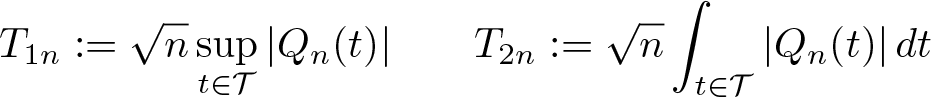
T_{1 n} : = \sqrt{n} \sup_{t \in T} | Q_{n} (t) | T_{2 n} : = \sqrt{n} \int_{t \in T} | Q_{n} (t) | d t

These statistics and their associated limiting theory provide a natural foundation for testing the null hypothesis. It is possible to formulate many tests using variants of the proposed tests. Note that inference for a single point estimation for a fixed level of treatment can be seen as a particular case of uniform inference with r(t) = q ₀ and $T = t$ . Alejo, Galvao, and Montes-Rojas (2018) show that simple hypotheses testing for fixed t can be based on Wald statistics.

For uniform inference for QCTE, we consider general null hypothesis

H_{0} : Δ_{τ}_{0} (t, t + δ) - s (t) = 0 t \in T

uniformly, where δ is a fixed treatment increment, s(t) is assumed to be known (continuous in t over T), and $s \in l^{\infty} (T)$ . Inference is carried uniformly over the set of treatment levels, T. The basic inference process is

D_{n} (t) : = {\hat{Δ}}_{τ} (t, t + δ) - s (t) t \in T

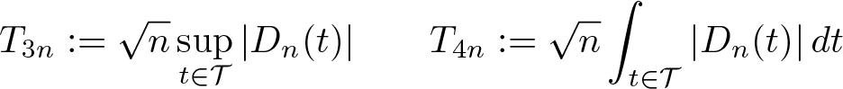
As before, we consider Kolmogorov–Smirnov and Cramér–von Mises test statistics, T_n = f{D_n (·)}, where f(·) represents the functionals for those two test statistics, as

T_{3 n} : = \sqrt{n} \sup_{t \in T} | D_{n} (t) | T_{4 n} : = \sqrt{n} \int_{t \in T} | D_{n} (t) | d t

Note that point inference for two different treatment values, say, t and t′, can be stated as a particular case with δ = t′ − t, r(t) = Δ₀, and $T = t$ . Again, the Wald statistic is valid in this particular case.

In practice, the procedure is implemented in a discretized subset, most conveniently on intervals of equal size, $T = [t_{1}, . . ., t_{m}], t_{1} < \dots < t_{m}$ . The weak limits of T _1n, T _2n, T _3n, and T _4n are functionals of Gaussian processes, and the estimation of their covariance kernel is difficult to compute. Therefore, to make practical inference, Alejo, Galvao, and Montes-Rojas (2018) suggest using simple bootstrap techniques to approximate the limiting distribution.

3 The qcte command

3.1 Syntax

The command syntax is

qcte depvar treatvar [ if ] [ in ] [ , xvar( varlist ) zvar( varlist ) t0( real ) t1( real )

dt( real ) quantile( # ) ynotrans reps( # ) nograph notest]

3.2 Options

xvar( varlist ) specifies the transformed control variables (Box–Cox model).

zvar( varlist ) specifies the nontransformed control variables.

t0( real ) sets the value of t ₀. The default is the first percentile of T.

t1( real ) sets the value of t ₁. The default is the last percentile of T.

dt( real ) sets the value of δ. The default is (t ₁ − t ₀)/19.

quantile( # ) specifies the quantile to estimate. The default is quantile(50).

ynotrans specifies to not transform the dependent variable.

reps( # ) specifies the number of bootstrap replications to be performed. The default is reps(50).

nograph suppresses the display of QDRF and QCTE plots.

notest suppresses the table display of statistics for uniform inference.

3.3 Stored results

qcte stores the following in r():

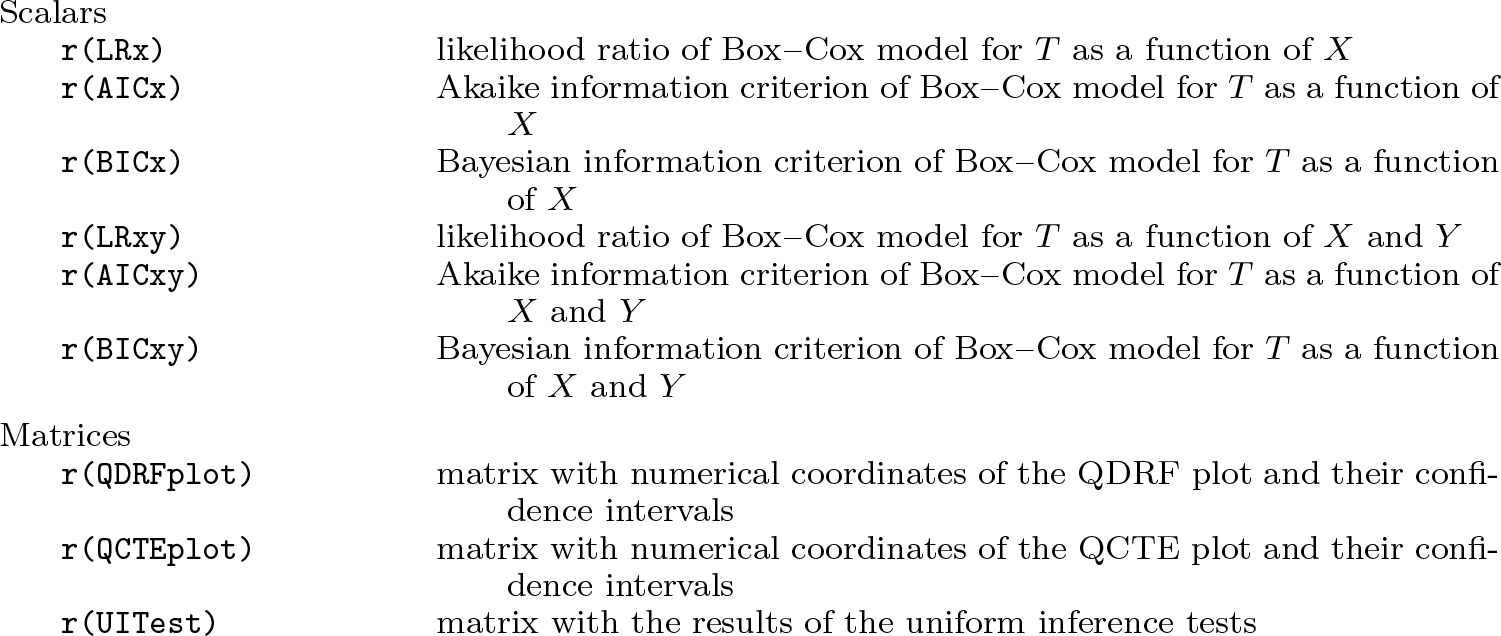
Matrices r(QDRFplot) and r(QCTEplot) are useful to replicate the output plot with other graph formats. r(UITest) stores the statistics T _1n, T _2n, T _3n, and T _4n, the critical values, and the p-values computed by bootstrap using r(t) = 0 and s(t) = 0.

4 Examples

In this section, we present the syntax of the qcte command, which implements the methodology suggested by Alejo, Galvao, and Montes-Rojas (2018) using two examples. First, we show some exercises with simulated data to show the basic output of the command on the screen. Second, we use qcte with real data using the base of winners of the lottery of Massachusetts.

4.1 Example 1: Simulations

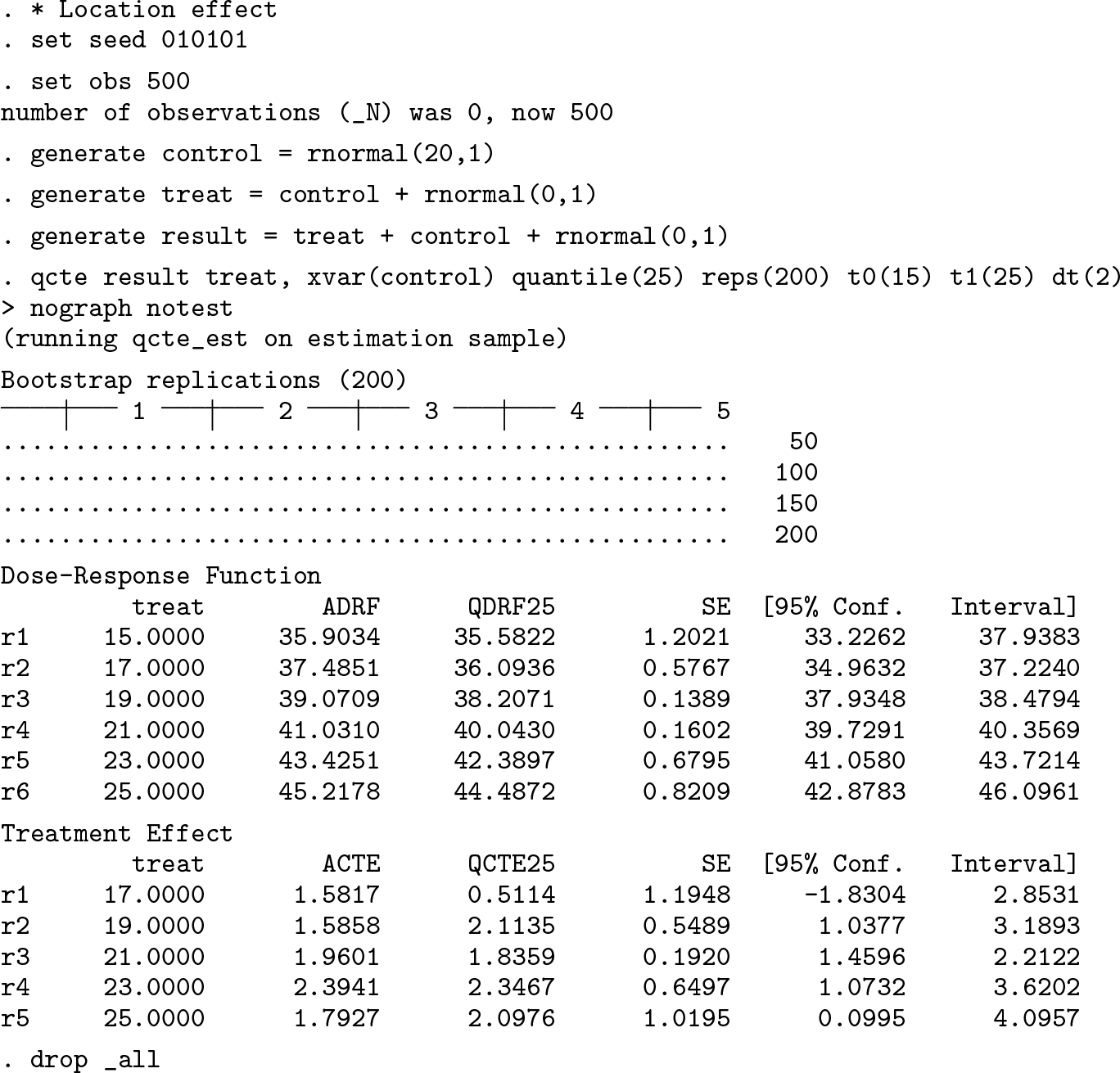
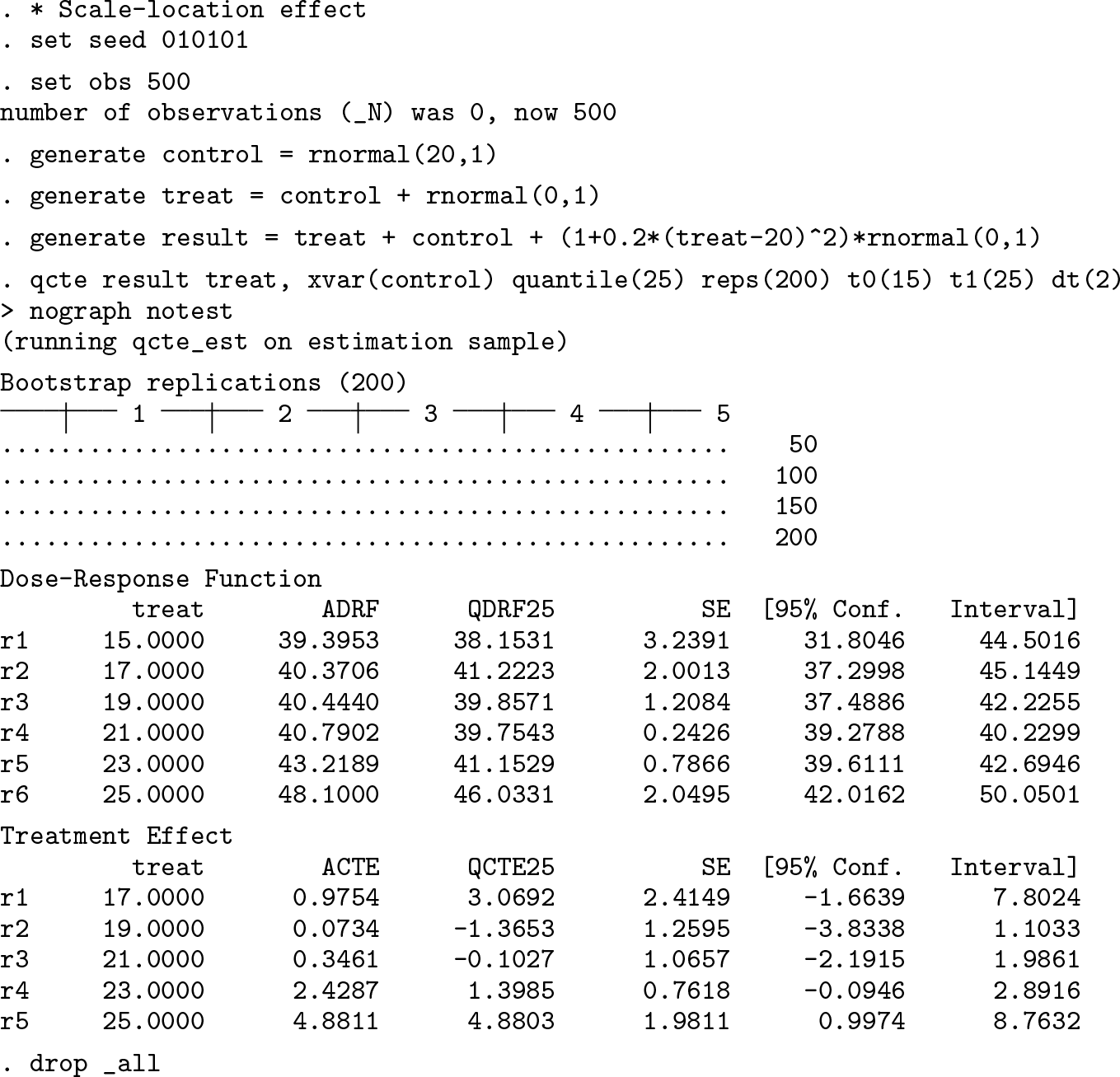
For comparison, we develop some examples in Alejo, Galvao, and Montes-Rojas (2018) by drawing random samples from data-generating processes: X = 20 + v ₁, T = X + v ₂, and Y = T + X + {1 + α(20 − t)²}v ₃ with v ₁, v ₂, and v ₃ independent random variables. The parameter α determines whether the treatment effect is a pure location shift (α = 0) or a scale-location shift α ≠ 0.

First, we evaluate the performance for a location shift treatment effect with standard normal distributions for v ₁, v ₂, and v ₃:

Second, we consider a random sample from a scale-location shift (α = 1/5) of the treatment with standard normal distributions for v ₁, v ₂, and v ₃:

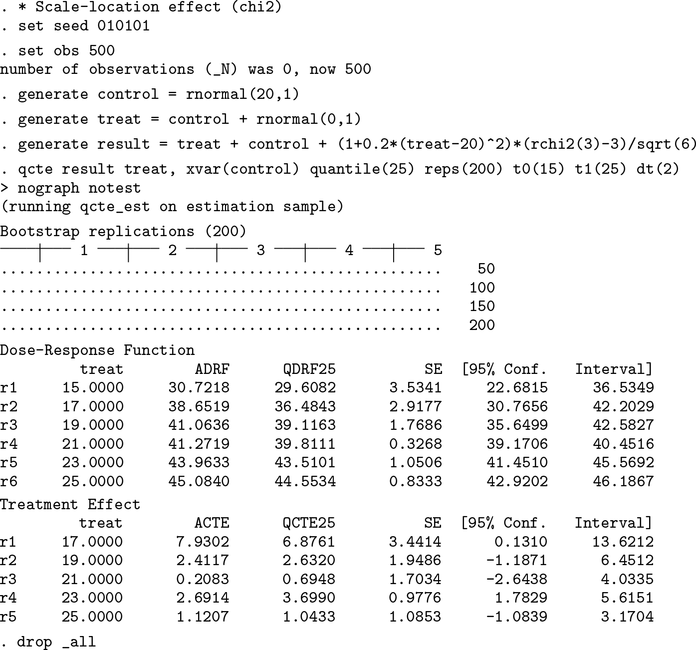
Third, we consider a scale-location shift model (α = 1/5) with a standardized $χ_{3}^{2}$ for v ₃. This case is characterized by the asymmetry due to a large mass of probability on the right tail of the distribution.

The output shows two tables: the top with the estimates for the dose–response function and the bottom for TE. Each treatment value is shown with its standard errors and the 95% confidence intervals computed via bootstrap. Note that in the three examples, we have set a grid of values for $T = {15, 17, \dots, 25}$ . By default, the QDRF in the output table is evaluated at 20 equidistant points between the first and last percentile of T . The estimated QCTE is the difference between each of the QDRF points. For simplicity, the plots and the uniform inference statistics have been omitted using options nograph and notest, respectively. The following example shows those command options.

4.2 Example 2: Real data

We illustrate the qcte command using the survey of Massachusetts lottery winners to estimate the effect of the prize amount (as a proxy of nonlabor income) on subsequent labor earnings from U.S. Social Security records. The prize amount is a continuous variable, so we apply the command to measure its effect on the quantiles of the distribution of earnings. This database is described in Imbens, Rubin, and Sacerdote (2001) and is also used as an empirical application in Hirano and Imbens (2004), Bia and Mattei (2008), and Bia et al. (2014) for estimating ADRF because the lottery prize is a continuous treatment variable.

Although the lottery prize is obviously randomly assigned, there is substantial correlation between some of the background variables and the lottery prize in our sample. The main source of potential bias is the unit and item nonresponse. In the survey, unit nonresponse was about 50%. To remove such biases, we make the weak unconfoundedness assumption that, conditional on covariates, the lottery prize is independent of the potential outcomes.

The sample we use in this analysis is the “winners” sample of 237 individuals who won a major prize in the lottery. For each individual, we observe social security earnings for six years before the lottery and six years after. The outcome of interest is year6 (earnings six years after winning the lottery), denoted Y, and the treatment is prize, the prize amount, denoted T . Control variables X are age, gender, years of high school, years of college, winning year, number of tickets bought, work status after winning, and earnings s years before winning the lottery (with s = 1, 2,…, 6). Of these 237 individuals, we keep a sample of 202 for whom we have income information on income Y . Detailed descriptive statistics can be found in Imbens, Rubin, and Sacerdote (2001) and Hirano and Imbens (2004).

As noted above, the correct estimation of the QDRF and QCTE models requires that the Box–Cox implementation in the first step produce consistent estimators of the conditional densities. After each model, the proposed command stores the Akaike information criterion and Bayesian information criterion values after each Box–Cox estimation. The user can use these goodness-of-fit measures as a guide to select a model specification. Appendix A.3 shows an example of model selection comparing some usual specifications with these goodness-of-fit measures. Below, we use the specification that emerges from that simple algorithm.

A feature of the data to be considered is that about half the sample has Y = 0 (52%, which corresponds to 47% for male and 59% for female). That is, about half the sample is not working and receives no income six years after winning the lottery. We follow Hirano and Imbens’s (2004) and Bia and Mattei’s (2008) approach, who consider that a zero value corresponds to an observed level of income and it requires no truncation analysis. 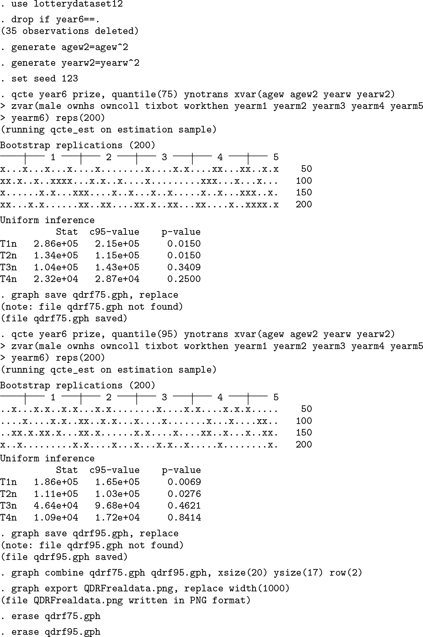We find that for low quantiles, that is, τ < 0.5, QDRF _τ (t) = 0, $\forall t \in T$ . Thus, we report only the QDRF for τ = 0.75, 0.95:

Figure 1 reports the ADRF with the QDRF for selected quantiles. The upper plot on the left corresponds to τ = 0.75 QDRF estimates, and the bottom plot on the left corresponds to τ = 0.95. The graph shows that Y (t) is a decreasing function of t, and the quantile analysis has the same shape as the average effects. As in Imbens, Rubin, and Sacerdote (2001), the effects show a convex relationship suggesting a marginally decreasing effect of the lottery prize on labor earnings.

Figure 1.

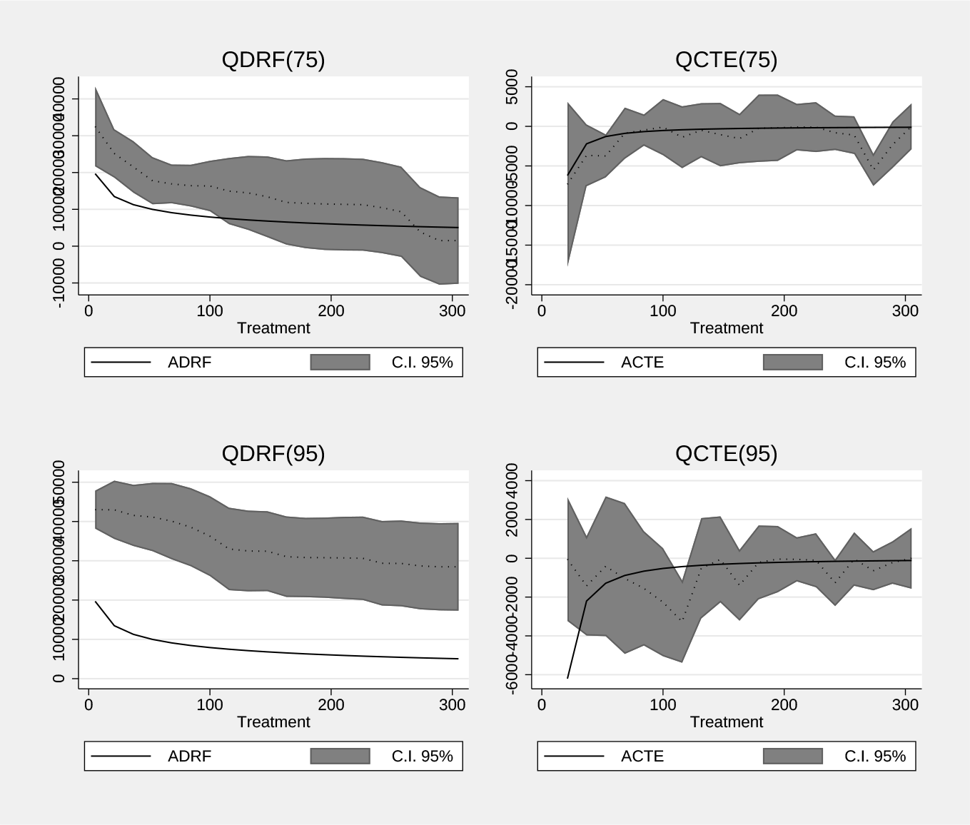
Empirical application: The Imbens–Rubin–Sacerdote lottery sample

Now consider inference on the point estimates and uniformly over the range of treatment values. The QDRF graph for τ = 0.75 shows that the estimates are different from 0 up to a treatment value of approximately 150 (that is, for those values of t, 0 is not included in the constructed confidence interval). The QDRF for τ = 0.95 and its 95% confidence interval are always above 0 for the entire treatment range. When we look at the uniform inference (T1n and T2n), the QDRF is different from zero uniformly throughout the evaluated range of treatment values for both τ = 0.75 and τ = 0.95. For the QCTE, the results in the graphs show that the effect of the amount won in the lottery has a nonzero treatment effect for only a few values of the continuous treatment variable. The uniform inference on QCTE (T3n and T4n), however, cannot reject the null of 0 QCTE for τ = 0.75, but it rejects the null hypothesis of 0 effect at the 5% level for τ = 0.95.

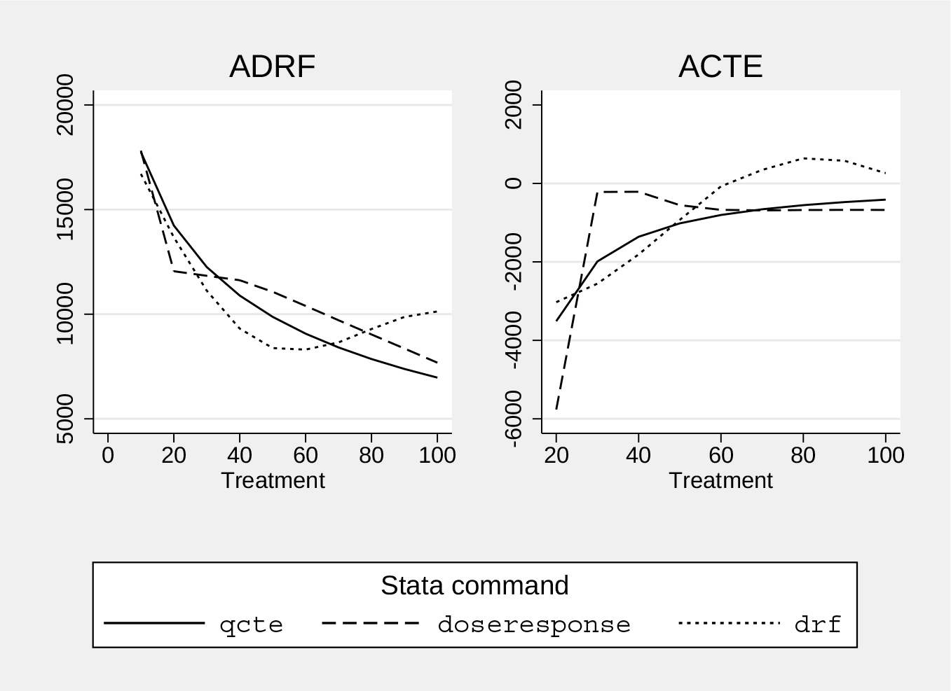
Finally, we compare the ADRF and ACTE estimated by our qcte command with those obtained using Bia and Mattei’s (2008) doseresponse command and Bia et al.’s (2014) drf command. For comparison, we use the same sample (prize below its 95th quantile) and range for T as in those articles. These two commands require the previous installation of the moremata package (see Jann [2005] and Bia et al. [2014]). The codes used to make the comparison are shown in appendix A.2. The results are shown in figure 2. Note that qcte estimates are smoother than the others and that they are in between the other two. Therefore, the average effects obtained with qcte are consistent with the previous commands for estimating ADRF and ACTE.

Figure 2.

Command comparison: Average values

5 Conclusion

In this article, we presented a new command, qcte, that estimates the quantile TE models with a continuous treatment by using a semiparametric two-step estimator suggested by Galvao and Wang (2015). Following Alejo, Galvao, and Montes-Rojas (2018), we used a simple Box–Cox model to compute the propensity score and a bootstrap approach to implement these methods for many testing procedures.

Our estimates replicated the results of Alejo, Galvao, and Montes-Rojas (2018) and showed that this convexity is homogeneous in the rest of the labor earnings distribution and then showed that the threshold value was monotonic in the quantiles. The application illustrated that this method is an important tool to study continuous TE. The quantile analysis also revealed that larger prizes produce lower labor earnings, but a larger prize is required for individuals in the upper part of the distribution of unobservables. The command also provided a graphical alternative to explore heterogeneity of a continuous treatment variable.

6 Programs and supplemental materials

Supplemental Material, st0597 - A practical generalized propensity-score estimator for quantile continuous treatment effects

Supplemental Material, st0597 for A practical generalized propensity-score estimator for quantile continuous treatment effects by Javier Alejo, Antonio F. Galvao and Gabriel Montes-Rojas in The Stata Journal

Footnotes

6 Programs and supplemental materials

To install a snapshot of the corresponding software files as they existed at the time of publication of this article, type

A Appendix

References

Abadie

Imbens

G. W.

2006. Large sample properties of matching estimators for average treatment effects. Econometrica 74: 235–267.

Alejo

Galvao

A. F.

Montes-Rojas

2018. Quantile continuous treatment effects . Econometrics and Statistics 8: 13–36. https://doi.org/10.1016/j.ecosta.2017.10.004.

Bia

Flores

C. A.

Flores-Lagunes

Mattei

2014. A Stata package for the application of semiparametric estimators of dose–response functions . Stata Journal 14: 580–604. https://doi.org/10.1177/1536867X1401400307.

Bia

Mattei

2008. A Stata package for the estimation of the dose–response function through adjustment for the generalized propensity score. Stata Journal 8: 354–373. https://doi.org/10.1177/1536867X0800800303.

Carroll

R. J.

Ruppert

1984. Power transformations when fitting theoretical models to data. Journal of the American Statistical Association 79: 321–328. https://doi.org/10.1080/01621459.1984.10478052.

Cattaneo

M. D.

2010. Efficient semiparametric estimation of multi-valued treatment effects under ignorability. Journal of Econometrics 155: 138–154. https://doi.org/10.1016/j.jeconom.2009.09.023.

Cattaneo

M. D.

Drukker

D. M.

Holland

A. D.

2013. Estimation of multivalued treatment effects under conditional independence. Stata Journal 13: 407–450. https://doi.org/10.1177/1536867X1301300301.

Chernozhukov

Hansen

2005. An IV model of quantile treatment effects. Econometrica 73: 245–261.

Cohen

1983. The cost of dichotomization. Applied Psychological Measurement 7: 249–253. https://doi.org/10.1177/014662168300700301.

10.

Cox

D. R.

1957. Note on grouping. Journal of the American Statistical Association 52: 543–547. https://doi.org/10.2307/2281704.

11.

Dehejia

R. H.

Wahba

1999. Causal effects in nonexperimental studies: Reevaluating the evaluation of training programs. Journal of the American Statistical Association 94: 1053–1062. https://doi.org/10.1080/01621459.1999.10473858.

12.

Fedorov

Mannino

Zhang

2009. Consequences of dichotomization. Pharmaceutical Statistics 8: 50–61. https://doi.org/10.1002/pst.331.

13.

Firpo

2007. Efficient semiparametric estimation of quantile treatment effects. Econometrica 75: 259–276.

14.

Flores

C. A.

2007. Estimation of dose–response functions and optimal doses with a continuous treatment. PhD dissertation, University of Miami. https://core.ac.uk/download/pdf/7169663.pdf.

15.

Flores

C. A.

Flores-Lagunes

Gonzalez

Neumann

T. C.

2012. Estimating the effects of length of exposure to instruction in a training program: The case of Job Corps. Review of Economics and Statistics 94: 153–171.

16.

Frölich

Melly

2010. Estimation of quantile treatment effects with Stata. Stata Journal 10: 423–457. https://doi.org/10.1177/1536867X1001000309.

17.

Galvao

A. F.

Wang

2015. Uniformly semiparametric efficient estimation of treatment effects with a continuous treatment. Journal of the American Statistical Association 110: 1528–1542. https://doi.org/10.1080/01621459.2014.978005.

18.

Hahn

1998. On the role of the propensity score in efficient semiparametric estimation of average treatment effects. Econometrica 66: 315–331.

19.

Hasebe

2013. Copula-based maximum-likelihood estimation of sample-selection models. Stata Journal 13: 547–573. https://doi.org/10.1177/1536867X1301300307.

20.

Heckman

J. J.

Ichimura

Smith

Todd

1998. Characterizing selection bias using experimental data. Econometrica 66: 1017–1098.

21.

Hirano

Imbens

G. W.

2004. The propensity score with continuous treatments. In Applied Bayesian Modeling and Causal Inference from Incomplete-Data Perspectives, ed. Gelman

Meng

X.-L.

, 73–84, 73–84. Chichester, UK: Wiley. https://doi.org/10.1002/0470090456.ch7.

22.

Hirano

Imbens

G. W.

Ridder

2003. Efficient estimation of average treatment effects using the estimated propensity score. Econometrica 71: 1161–1189.

23.

Imai

van Dyk

D. A.

2004. Causal inference with general treatment regimes: Generalizing the propensity score. Journal of the American Statistical Association 99: 854–866.

24.

Imbens

G. W.

2000. The role of the propensity score in estimating dose–response functions. Biometrika 87: 706–710.

25.

Imbens

G. W.

Rubin

D. B.

Sacerdote

B. I.

2001. Estimating the effect of unearned income on labor earnings, savings, and consumption: Evidence from a survey of lottery players. American Economic Review 91: 778–794.

26.

Jann

2005. moremata: Stata module (Mata) to provide various functions. Statistical Software Components S455001, Department of Economics, Boston College. https://ideas.repec.org/c/boc/bocode/s455001.html.

27.

Koenker

Bassett

Jr.

1978. Regression quantiles. Econometrica 46: 33–50.

28.

Lechner

2001. Identification and estimation of causal effects of multiple treatments under the conditional independence assumption. In Econometric Evaluation of Labour Market Policies, ed. Lechner

Pfeiffer

. 43–58, 43–58. Heidelberg: Physica-Verlag.

29.

Lee

2018. Partial mean processes with generated regressors: Continuous treatment effects and nonseparable models. Department of Economics, University of California– Irvine. https://arxiv.org/abs/1811.00157.

30.

Racine

J. S.

Wooldridge

J. M.

2009. Efficient estimation of average treatment effects with mixed categorical and continuous data. Journal of Business & Economic Statistics 27: 206–223.

31.

Rubin

D. B.

1977. Formalizing subjective notions about the effect of nonrespondents in sample surveys. Journal of the American Statistical Association 72: 538–543.

32.

van Belle

2008. Statistical Rules of Thumb. 2nd ed. Hoboken, NJ: Wiley.

Supplementary Material

Please find the following supplemental material available below.

For Open Access articles published under a Creative Commons License, all supplemental material carries the same license as the article it is associated with.

For non-Open Access articles published, all supplemental material carries a non-exclusive license, and permission requests for re-use of supplemental material or any part of supplemental material shall be sent directly to the copyright owner as specified in the copyright notice associated with the article.

0.01 MB

0.00 MB

A practical generalized propensity-score estimator for quantile continuous treatment effects

Abstract

Keywords

1 Introduction

2 Continuous treatment effects

2.1 Two-step estimator

First step: Estimation of w 0

Second step: Estimation of qτ 0 and Δ τ 0

2.2 Inference procedures

3 The qcte command

3.1 Syntax

3.2 Options

3.3 Stored results

4 Examples

4.1 Example 1: Simulations

4.2 Example 2: Real data

5 Conclusion

6 Programs and supplemental materials

Supplemental Material, st0597 - A practical generalized propensity-score estimator for quantile continuous treatment effects

Footnotes

6 Programs and supplemental materials

A Appendix

References

Supplementary Material

First step: Estimation of w ₀

Second step: Estimation of q_τ ₀ and Δ _τ ₀