Sage Journals: Discover world-class research

Abstract

Recognizing a dose–response pattern based on heterogeneous tables of contrasts is hard. Specification of a statistical model that can consider the possible dose–response data-generating mechanism, including its variation across studies, is crucial for statistical inference. The aim of this article is to increase the understanding of mixed-effects dose–response models suitable for tables of correlated estimates. One can use the command drmeta with additive (mean difference) and multiplicative (odds ratios, hazard ratios) measures of association. The postestimation command drmeta_graph greatly facilitates the visualization of predicted average and study-specific dose–response relationships. I illustrate applications of the drmeta command with regression splines in experimental and observational data based on nonlinear and random-effects data-generation mechanisms that can be encountered in health-related sciences.

Keywords

st0638 drmeta drmeta_graph drmeta_gof predict after drmeta meta-analysis meta-regression mixed effects summarized data dose–response

1 Introduction

Investigating dose–response relationships underlying tables of empirical findings has become extremely popular in several research disciplines such as oncology, cardiology, endocrinology, nutrition, and public environmental health. The number of published dose–response meta-analyses increased exponentially over the last 15 years. Scatterplots of collected data are frequently used to inform the specification of the dose–response model. It is unlikely, however, that naked eyes can recognize a clear dose–response pattern. The meta-analyst has to face a limited number of estimates within each study, positive covariance of these estimates, diverse modeling choices of the quantitative dose, and sampling errors that may vary considerably across studies. Also, innumerable assumptions arise from the research environment of each study. In most applications, it is unreasonable to expect that a single dose–response mechanism operates equally in all the studies.

To be concrete, I present an example of data available to the meta-analyst in table 1. Distinct features of these types of data are that estimated contrasts within each study are relative to a common referent; the common referent may change across studies; estimated variances (standard errors) of the contrasts are available from the confidence intervals (CIs), but their covariances are missing; the single value of the dose corresponding to each estimated contrast is the typical dose observed in the sample (that is, the sample mean and median); the reference value of the dose can be far away from zero; and some descriptive statistics are usually available for each dose (that is, the sample standard deviation of the outcome, sample size, and number of cases).

Table 1.

Example of summarized dose–response data (mean dose within each quantile, estimated mean outcome difference and its standard error, sample standard deviation, and sample size) arising from five experimental studies

Study	Dose	Mean difference	Standard error	Standard deviation	Size
1	2.09	0.00	0.00	10.20	667
1	4.42	−1.83	0.54	9.63	667
1	8.50	−0.71	0.57	10.63	666
2	2.09	0.00	0.00	10.02	334
2	4.35	−2.24	0.79	10.39	333
2	8.57	4.00	0.84	11.56	333
4	2.66	0.00	0.00	9.97	1000
4	7.33	−1.90	0.45	10.25	1000
7	1.98	0.00	0.00	9.98	167
7	4.24	2.22	1.11	10.25	167
7	8.40	19.95	2.31	28.08	166
10	2.63	0.00	0.00	10.14	1000
10	7.30	6.01	0.55	13.95	1000

Traditionally, these types of data are analyzed using a two-stage approach (Orsini and Spiegelman 2020). A dose–response model is first fit within each study using generalized least squares (GLS) (Berrington and Cox 2003; Orsini, Bellocco, and Greenland 2006), and then estimates are combined across studies using multivariate random-effects meta-analysis (White 2009; Jackson, Riley, and White 2011). A one-stage approach for dose–response meta-analysis has been proposed to avoid exclusions of studies that do not provide enough data points to estimate the hypothesized functional relationship (Crippa et al. 2019).

Although any attempt to find a clear dose–response signal in the noisy estimates may appear worthless, the aim of this article is to increase the understanding of a one-stage approach, essentially a mixed-effects framework for meta-analysis (Sera et al. 2019), to evaluate what dose–response mechanism might be underlying multiple tables of correlated contrasts.

The article is organized as follows: explanation of weighted mixed-effects dose– response models including estimation, hypothesis testing, and predictions (section 2); description of the syntax of the drmeta command and its postestimation commands (section 4); application of the model to simulated examples from nonlinear and randomeffects data-generating mechanisms (section 4); and conclusion with some final remarks (section 9).

2 Methods

Depending on the study design and regression model used to analyze individual data, the dependent variable ${\hat{γ}}_{i}$ represents additive (mean difference, standardized mean difference) or multiplicative (log odds-ratio, log risk-ratio, log hazard-ratio) measures of association.

2.1 Weighted mixed-effects dose–response model

A weighted (linear) mixed-effects dose–response model (Crippa et al. 2019) can be specified as

{\hat{γ}}_{i} = X_{i} β + Z_{i} b_{i} + ϵ_{i}

where ${\hat{γ}}_{i}$ is a set of differences in predicted responses relative to a reference dose x_i ₀

for the ith study. The fixed-effects β define the average or summary dose–response relationship of the population of studies of which I occurred to be observed. A distinct feature of this mixed model is the absence of an intercept in X _i . The consequence is that the fitted curve within each study has to go, as it should, through the study-specific origin. The design matrix X _i , similarly to the dependent variable ${\hat{γ}}_{i}$ , is centered on the study-specific referent.

Suggestions on how to model the dose–response relationship are presented in section 2.2. When modeling the dose with transformations such as fractional polynomials or splines, there will be p transformations of the dose defining the design matrix.

The random-effects b _i represent study-specific deviations from the average regression coefficients β. Random-effects b _i are assumed to follow a multivariate normal distribution MVN (0, Ψ). The matrix Z _i is the analogous design matrix for the unobserved random effects. Of note, because the fixed effects jointly define the shape of the average dose–response relationship, random effects are placed on either all the regression coefficients or none of them. A random-effects model recognizes the presence of a distribution of possible true dose–response relationships that can be described in terms of central tendency and spread across studies.

The residual error term ϵ_i follows MVN (0, S _i ) with a variance–covariance matrix S _i that is assumed known in the sense that S _i has been already estimated (inverse Fisher information) together with ${\hat{γ}}_{i}$ . The matrix S _i can be available to the meta-analyst directly from the principal investigator of each study or, more commonly, approximated using algorithms based on a mix of available descriptive and inferential statistics (Greenland and Longnecker 1992; Hamling et al. 2008; Orsini et al. 2012; Crippa and Orsini 2016). The matrix S _i is important because it defines the weights to be used for each study. Every study-specific set of empirical estimates is weighted by the inverse of its estimated variance–covariance matrix.

The marginal model of (1) can be written as

{\hat{γ}}_{i} ~ N (X_{i} β, Z_{i} Ψ Z_{i}^{⊤} + S_{i})

with $Z_{i} Ψ Z_{i}^{⊤} + S_{i} = Σ_{i}$ . The marginal variance Σ _i can be separated into two parts: the within-study weights S _i and the between-study variability Ψ.

2.2 Possible dose–response functions

The quantitative dose should be modeled according to the possible dose–response datagenerating mechanism and the questions the meta-analyst is willing to ask in light of the available knowledge. For example, questions about the extent to which data are compatible with a threshold effect may be articulated differently: Compared with doses below the value k, what is the change in response for values of the dose above k? What is the rate of change in response below and above the value of k? What is the value of the dose k associated with the lowest response without imposing any specific functional relationship on the data?

The meta-analyst can imagine a variety of dose transformations to capture the main features of the true dose–response mechanism and at the same time answer the specified research questions. Below, we specify a few possible dose–response functions involving only one or two regression coefficients.

Linear function

The question is, What is the constant change in response associated with every one-unit increase of the dose? The weighted mixed-effects model using a linear function (M_l ) can be written as follows:

{\hat{γ}}_{i j} = (β_{1} + b_{1 i}) x_{i j} + ϵ_{i j}

Piecewise constant function

The question is, What is the sudden change in response after the knot k? A degree-0 spline of the dose x_ij is defined by the location of the knot k. The weighted mixed-effects model using a constant spline function (M_c ) can be written as

{\hat{γ}}_{i j} = (β_{1} + b_{1 i}) x_{i j} + (β_{2} + b_{2 i}) I (x_{i j} > k) + ϵ_{i j}

where the regression coefficient of the degree-0 spline β ₂ is the vertical shift in response after the knot k.

Piecewise cubic spline function

The question is, What is the smooth change in response along the range of the observed dose without imposing any specific shape? Linearity constraints are usually placed before the first knot and above the last knot to reduce the number of regression coefficients and increase stability at the tails of the dose distribution (Harrell 2001, Orsini and Greenland 2011).

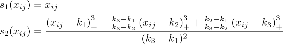
The weighted mixed-effects model using a restricted cubic spline function (M_s ) can be written as

{\hat{γ}}_{i j} = (β_{1} + b_{1 i}) s_{1} (x_{i j}) + (β_{2} + b_{2 i}) s_{2} (x_{i j}) + ϵ_{i j}

with three knots (k ₁ , k ₂ , k ₃) typically located at fixed percentiles of the dose distribution. The two splines are

\begin{array}{l} s_{1} (x_{i j}) = x_{i j} \\ s_{2} (x_{i j}) = \frac{{(x_{i j} - k_{1})}_{+}^{3} - \frac{k_{3} - k_{1}}{k_{3} - k_{2}} {(x_{i j} - k_{2})}_{+}^{3} + \frac{k_{2} - k_{1}}{k_{3} - k_{2}} {(x_{i j} - k_{3})}_{+}^{3}}{{(k_{3} - k_{1})}^{2}} \end{array}

A visualization of the fitted model is necessary to interpret the dose–response relationship.

Piecewise linear function

The question is, What is the constant change in response associated with every one-unit increase in the dose before and after the knot k? The weighted mixed-effects model using a linear spline function (M_p ) can be written as

{\hat{γ}}_{i j} = (β_{1} + b_{1 i}) x_{i j} + (β_{2} + b_{2 i}) I (x_{i j} > k) (x_{i j} - k) + ϵ_{i j}

where the regression coefficient of the degree-1 spline β ₂ is the change in linear trend after the knot k.

2.3 Estimation

We consider estimation methods based on maximum likelihood (ML). The marginal log likelihood of the weighted mixed-effects model (1) to be maximized with respect to the parameters of interest [p fixed effects plus q = p(p + 1)/2 variances–covariances of the random effects] given the I tables of aggregated data is defined as

\begin{array}{l} l (β, ξ) = - \frac{1}{2} n \log (2 π) - \frac{1}{2} \sum_{i = 1}^{I} \log | Σ_{i} (ξ) | + \\ - \frac{1}{2} \sum_{i = 1}^{I} {{({\hat{γ}}_{i} - X_{i} β)}^{⊤} Σ_{i} {(ξ)}^{- 1} ({\hat{γ}}_{i} - X_{i} β)} \end{array}

where $n = \sum_{i = 1}^{I} (J_{i} - 1)$ and ξ is the vector of the variance–covariance components in Ψ to be estimated. The maximized log likelihood can be used to compare alternative dose–response models using the Akaike information criterion (AIC) = −2ℓ+2(p+q), with p and q indicating the number of fixed and variance–covariance components, respectively (Müller, Scealy, and Welsh 2013).

ML estimates of the variance components have been shown to be biased downwards because of estimation of the fixed-effects β. An alternative is provided by restricted maximum-likelihood (REML) estimation that maximizes the likelihood

\begin{array}{r} l_{R} (ξ) = - \frac{1}{2} (n - p) \log (2 π) - \frac{1}{2} \sum_{i = 1}^{I} \log | Σ_{i} (ξ) | - \frac{1}{2} \log | \sum_{i = 1}^{I} X_{i}^{⊤} {Σ_{i} (ξ)}^{- 1} X_{i} | + \\ - \frac{1}{2} \sum_{i = 1}^{I} [{({\hat{γ}}_{i} - X_{i} \hat{β})}^{⊤} {Σ_{i} (ξ)}^{- 1} ({\hat{γ}}_{i} - X_{i} \hat{β})] \end{array}

where $\hat{β}$ indicates the estimates obtained by GLS. Both ML and REML estimation methods have been implemented in the drmeta command. The common-effects analysis constrains the variance components ξ in Ψ to be all equal to 0.

2.4 Hypothesis testing

Hypothesis testing and CIs for linear combinations of regression coefficients and data can be constructed using standard large-sample statistical inference from mixed models. The average dose–response curve is defined by the regression coefficients β. A test of the hypothesis H ₀ : β = 0 versus H_A : β ≠ 0 can be based on the Wald-type statistic

W = \hat{β} V {(\hat{β})}^{- 1} {\hat{β}}^{'}

using the estimated $\hat{β}$ and its variance–covariance matrix $V (\hat{β})$ . Assuming the null hypothesis is true, the observed p-value is obtained by reference to a χ ² distribution with p degrees of freedom. In the case of one regression coefficient, the Wald-type statistic $z = \hat{β} / \sqrt{V (\hat{β})}$ is compared with a standard normal distribution and typically shown in the output.

Depending on the functional form specified, testing part of the regression coefficients may detect specific characteristics of the shape (that is, nonlinearity, shift in level, change in slope). This can be done by testing H ₀ : β^∗ = 0, where β^∗ refers to the subset of coefficients defining those characteristics. For example, if the dose has been modeled using restricted cubic spline models with three knots (two splines), a p-value detecting departure from a simpler straight line can be obtained by testing the coefficient of the second spline equal to 0.

2.5 Prediction

Estimating the average or summary dose–response relationship is an important step, particularly when moving beyond straight lines, to present the results in tabular and in graphical form. Let x ^∗ be the (v × p) design matrix obtained by applying the chosen dose–response function (see section 2.2) to a number v of plausible values of the dose, and let x ₀ ^∗ be the same design matrix evaluated at the chosen reference level. The rationale for using x ^∗ rather than the observed X _i used to fit the model is that X _i does not contain enough data points for a smooth plot of either the average or the study-specific dose–response relationship. The (v×1) vector of predicted average changes in responses is given by

{\hat{γ}}^{*} = (x^{*} - x_{0}^{*}) \hat{β}

with pointwise 100(1 − α)% CIs obtained as follows:

(x^{*} - x_{0}^{*}) \hat{β} \pm z_{α / 2} diag {(x^{*} - x_{0}^{*}) V (\hat{β}) {(x^{*} - x_{0}^{*})}^{⊤}}^{1 / 2}

The estimated values of ${\hat{γ}}^{*}$ represent pointwise, dose x ^∗ versus $x_{0}^{*}$ , average differences in means, log risks, log odds, or log rates depending on the type of measure being modeled. Using the invariance property of ML estimates, we obtain inference on multiplicative measures of association by exponentiating the point and interval estimates defined above.

An advantage of the mixed-effects model is that it allows estimation of study-specific dose–response relationships. The best linear unbiased prediction (BLUP) of b can be computed as

{\hat{b}}_{i} = \hat{Ψ} Z_{i}^{⊤} {\hat{Σ}}_{i}^{- 1} ({\hat{γ}}_{i} - X_{i} \hat{β})

The conditional study-specific dose–response relationships are obtained by adding the fixed effects and BLUPs as follows:

{\hat{γ}}_{i}^{*} = (x^{*} - x_{0}^{*}) (\hat{β} + {\hat{b}}_{i})

Overlaying the average ${\hat{γ}}^{*}$ and study-specific ${\hat{γ}}_{i}^{*}$ allows visual appreciation of the central tendency and spread of dose–response relationships across studies.

3 The commands

3.1 drmeta

drmeta fits parametric dose–response models based on tables of correlated contrasts. It fits fixed-effects and random-effects mixed models using a one-stage or a two-stage approach. Measures of association include odds ratios, risk ratios, hazard ratios, mean differences, and standardized mean differences.

Syntax

drmeta depvar dose_vars [ if ] [ in ] [ , se( varname ) data( varname1 varname2 ) id( varname ) type( varname ) or rr hr md smd vwls 2stage ml reml hamling acov( varname ) mcov( matrix_list ) noretable stddeviations nolrt eform level( # )]

After drmeta, specific postestimation commands are drmeta_graph, drmeta_gof, and predict.

Options

se( varname ) specifies an estimate of the standard error of depvar.

data( varname1 varname2 ) specifies variables containing the information required to

reconstruct the covariances of depvar. At each exposure level, varname1 is the number of subjects (controls plus cases) if depvar is (log) odds ratios; the total person-time if depvar is (log) hazard ratios; or the total number of persons (cases plus noncases) if depvar is (log) risk ratios. The variable varname2 contains the number of cases at each exposure level. If depvar is mean differences and standardized mean differences total, the variable varname1 indicates the total number of persons, and the variable varname2 contains the standard deviation of the outcome at each exposure level. Any missing values in either of the two variables set the covariances to 0.

id( varname ) specifies the variable identifying study-specific contrasts. The reference dose is the row with a value of 0 for the standard error. This option is required with multiple studies.

type( varname ) specifies the variable indicating the type of measure used to contrast dose levels. It can take on value 1 for odds ratios, 2 for hazard ratios, 3 for risk ratios, 4 for mean differences, and 5 for standardized mean differences.

or specifies that depvar be (log) odds ratios. It is used for dose–response estimation for a single study. It is not necessary if the option id( varname ) is specified.

rr specifies that depvar be (log) risk ratios. It is used for dose–response estimation for a single study. It is not necessary if the option id( varname ) is specified.

hr specifies that depvar be (log) hazard ratios. It is used for dose–response estimation for a single study. It is not necessary if the option id( varname ) is specified.

md specifies that depvar be mean differences. It is used for dose–response estimation for a single study. It is not necessary if the option id( varname ) is specified.

smd specifies that depvar be standardized mean differences. It is used for dose–response estimation for a single study. It is not necessary if the option id( varname ) is specified.

vwls sets the covariances of depvar within each study to 0.

2stage specifies the two-stage approach for dose–response meta-analysis. It calls the

mvmeta command. The default is the one-stage approach.

ml fits a random-effects model via ML; this is the default. All variances and covariances of the random effects are allowed to be distinct. So if dose_vars includes p variables, then additional p(p + 1)/2 random-effects parameters are estimated.

reml fits a random-effects model via REML. All variances and covariances of the random effects are allowed to be distinct. So if dose_vars includes p variables, then additional p(p + 1)/2 random-effects parameters are estimated.

hamling specifies the Hamling method (Hamling et al. 2008) to estimate the covariances when depvar is a log relative-risk. The default is the Greenland and Longnecker method (Greenland and Longnecker 1992; Orsini, Bellocco, and Greenland 2006). When depvar is a mean difference or a standardized mean difference, the method used for the covariance is described by Crippa and Orsini (2016).

acov( varname ) passes the average covariance as a variable.

mcov( matrix_list ) passes a list of variance–covariance matrices, one for each study. It is an advanced option where the order of the matrix list matters. The first matrix is supposed to be related to the first set of contrasts and so on. It can be useful when empirical contrasts and related variance–covariance matrices are available directly from fitting a model on primary data. So this option allows the user to skip the specification of the data() option.

noretable suppresses the random-effects parameter estimates.

stddeviations displays the random-effects and residual-error parameter estimates as standard deviations and correlations.

Nolrt suppresses the likelihood-ratio test for the unstructured variance–covariance components. It assesses whether all random-effects parameters of the dose–response model are simultaneously zero. Of note, the likelihood-ratio test is conservative.

eform reports coefficient estimates as exp(b) rather than b. Standard errors and CIs are similarly transformed.

level( # ) sets the confidence level, as a percentage, for CIs. The default is level(95) or as set by set level.

Stored results

drmeta stores the following in e():

3.2 drmeta_graph

The drmeta_graph command greatly facilitates the estimation and presentation of the average and study-specific dose–response relationships using a common referent. The drmeta_graph command tabulates and plots the average dose–response relationship together with CIs upon indication of a list of dose values, a referent, and the types of transformations used to model the quantitative dose. It is particularly convenient when modeling the dose with spline transformations.

Syntax

drmeta_graph [ , dose( numlist ) ref( # ) equation( string ) matknots( matname ) knots( numlist ) blup gls level( # ) eform scatter list addplot( string ) plotopts( string ) format(% fmt ) twoway_options ]

Options

dose( numlist ) specifies the values of the dose at which to estimate differences in predicted responses.

ref( # ) specifies the reference value of the dose; this value is not necessarily included in dose( numlist ).

equation( string ) specifies the mathematical transformations of the dose d used in the previously fitted dose–response model. It is relevant only if matknots( matname ) or knots( numlist ) has not been specified. Example 1: equation( d ) means that the dose was modeled assuming a linear function. Example 2: equation( d d ² ) means that the dose was modeled with a quadratic function. Example 3: equation( d ln(d)) means that the dose was modeled with d and the natural logarithm of d.

matknots( matname ) specifies the matrix of knots used to create restricted cubic splines. This can be easily obtained from the stored results of the mkspline command.

knots( numlist ) specifies a list of knots used to create the restricted cubic splines. It is an alternative to the option matknots( matname ).

blup shows conditional study-specific lines arising from the estimated random-effects model (best linear unbiased prediction).

gls shows study-specific lines estimated separately using GLS.

level( # ) sets the confidence level as a percentage for CIs. The default is level(95) or as set by set level.

eform exponentiates the estimated differences in predicted responses.

scatter shows a scatterplot rather than a line plot (default).

list lists the estimated differences in predicted responses.

addplot( string ) specifies the equation of the model to be plotted in terms of the dose d. It can be useful to overlay a line or curve on the graph of the previously fitted model. Example 1: You previously fit a spline model, and you want to add a line addplot( b_1 ∗ (d − 10)), representing the change in predicted outcome relative to the dose value of 10 according to a linear function. Example 2: You previously fit a linear response model, and you want to add a curve addplot( b_1 ∗ (d − 10) + b_2 ∗ (d ² − 100)), representing the change in predicted outcome relative to the dose value of 10 according to a quadratic function.

plotopts( string ) controls the line options affecting the added plot with the option addplot( string ).

format(% fmt ) specifies the display format for presenting numbers. format(%3.2f) is the default; see help format.

twoway_options are most of the options documented in [G] twoway_options , including options for titles, axes, labels, schemes, and saving the graph to disk. However, the by() option is not allowed.

3.3 drmeta_gof

The drmeta_gof command provides tools (deviance test, R ²) to evaluate the goodness of fit in dose–response meta-analysis (Discacciati, Crippa, and Orsini 2017). It is a postestimation tool of the drmeta command.

Syntax

drmeta_gof [ , r2s opvdplot( dose_var , [ xb | xbs | fitted[) drvdplot( dose_var )

dovpplot twoway_options ]

Options

r2s shows the study-specific coefficient of determination (R ²).

opvdplot( dose_var , [ xb | xbs | fitted[) plots the observed and specified predicted values versus the specified dose. The default is to use study-specific predictions using GLS (xbs). See section 3.4.

drvdplot( dose_var ) plots the decorrelated residuals versus the specified dose.

dovpplot plots decorrelated observed contrasts versus predicted contrasts.

twoway_options are most of the options documented in [G] twoway_options, including

options for titles, axes, labels, schemes, and saving the graph to disk. However, the by() option is not allowed.

3.4 predict

The postestimation command predict after drmeta creates a new variable containing the requested predictions using study-specific reference values.

Syntax

predict stubname [ , xb xbs fitted reffects]

Options

xb calculates the linear prediction for the fixed portion of the model only; this option is the default.

xbs calculates the linear prediction using a study-specific coefficient vector estimated using GLS.

fitted calculates fitted values, that is, a fixed-portion linear prediction plus contributions based on predicted random effects.

reffects predicts BLUPs of random effects.

4 Examples

Weighted mixed-effects models are illustrated using three examples based on tables of mean differences, odds ratios, and hazard ratios estimated from nonlinear and random-effects data-generating mechanisms. Tables are generated using a Monte Carlo simulation. Knowing the values of the parameters that govern the central tendency and spread of the dose–response relationships across studies helps to evaluate the results obtained in any given sample of studies.

4.1 Tables of mean differences

Consider the tables of summarized data from 10 hypothetical studies investigating the association between a quantitative dose and a quantitative outcome. The dose, randomly assigned to each individual, is positive and skewed to the right (χ ² with 5 degrees of freedom). Each principal investigator has categorized the quantitative dose into quantiles and conducted statistical inference on differences in population mean outcomes across quantiles of the dose using a linear regression model. The 10 studies are sampled from a random-effects nonlinear data-generating mechanism. We simulated a J-shaped [−2(x − 5) + 0.2(x ² − 5²)] dose–response relationship for the average study. Given this shape, the lowest mean outcome is expected to be at the mean dose of x = −(−2)/{2(0.2)} = 5 units. There is no single true dose–response relationship underlying all the studies. Every study provided an estimate of its own true dose–response relationship with a certain sampling error. The inferential objective of the meta-analyst can be to determine the tendency and spread of all of these true dose–response relationships. The empirical estimates and descriptive statistics obtained by the study investigators are useful to the extent they can contribute to the understanding of the features of the distribution of dose–response relationships.

Let’s pretend we do not know the data-generating mechanism described above. The 10 observed studies vary according to sample size, dose categorization, and mean dose of the reference category. A total of 13,500 individuals have been involved in these studies contributing to the estimation of 24 mean outcome differences. Moving away from the bottom category of the dose (about 2 units), some studies estimated a lower mean outcome, some other studies a higher mean outcome, and some studies no substantial change (figure 1). The visual impression is of a large variation in the dose–response association across studies.

Figure 1.

Graph of the study-specific estimated mean differences (95% CIs, capped spikes) arising from 10 studies of different sizes. Marker size is inversely related to its variance. The shaded area is the distribution of the dose in the population.

It can be hard for the meta-analyst to imagine what kind of functional relationship might be underlying these tables of empirical estimates if the only knowledge available is the collected data. For simplicity of analysis and interpretation, a common strategy used by meta-analysts is a linear function (M_l ) for the dose.

Every one-unit increase of the dose is estimated to increase, on average, the mean outcome by ${\hat{β}}_{1} = 0.31$ units (95% CI: [−0.41, 1.04]). The estimated variance of the random effects is large, suggesting a strong variability of the study-specific linear trends. Data appear to be compatible with a flat dose–response association (z = 0.85, p-value = 0.394). To some health researchers, a linear association with a large p-value, strong heterogeneity, and no clear visual pattern in the estimates may discourage further analysis and could be the beginning of stratified analysis, quality analysis, and wondering about possible explanations for these heterogeneous observed data. Although we cannot exclude that the dose–response relationship can be actually linear for some studies, data may also be compatible with the hypothesis of higher mean outcomes at the dose extremes relative to the middle range of the dose (that is, U/J-shaped). Such a shape would be unlikely to be discovered by forcing a linear dose–response function in all the studies. Therefore, we now allow a curvilinear relationship to be detected using restricted cubic splines with three knots of the dose (M_s ). When the likelihood of the table of empirical estimates using a spline function is much larger than the ones obtained with the linear function, there would be an indication of departure from a linear function. Because the linear function is a special case of the restricted cubic spline function, one could also test the compatibility of the data with a simpler linear function testing the hypothesis that the regression coefficient of the second spline is equal to 0. The result of the Wald-type test is shown in the output below.

The maximized log likelihood of a mixed-effects model using the restricted cubic spline function (ℓ_s = −49) of the dose is, in absolute terms, about two-fifths of the maximized log likelihood of the linear function (ℓ_l = −118). Even considering the higher number of estimated parameters of the spline function (two coefficients + three variance–covariance of random effects) relative to the linear function (one coefficient + one variance of random effects), the AIC of the spline function (AIC _s = 107) is about half the one of the linear function (AIC _l = 240). Assuming the average dose–response function is truly linear, a Wald-type statistic being as or more extreme than observed would rarely occur (H ₀ : β ₂ = 0, z = 5.24, p-value < 0.001). That said, we still have no idea of the possible shape relating the dose to the mean outcome. Therefore, we next present graphically the estimated summary dose–response relationship using the overall dose of five units as referent (figure 2).

Figure 2.

Estimated summary dose–response relationship (solid line) with 95% CIs (short-dashed lines) based on 10 tables of empirical estimates. Data were fit with a weighted mixed-effects model using restricted cubic splines for the dose with three knots located at percentiles (10th, 50th, 90th) of the overall dose distribution. The long-dashed line is the true summary dose–response relationship. The dose value of five units served as a referent.

Based on the spline model, the predicted summary mean outcome difference comparing the generic dose level x^∗ versus the reference of five units, compactly indicated with ${\hat{γ}}_{x^{*}, 5}^{*}$ , is given by

{\hat{γ}}_{x^{*}, 5}^{*} = - 1.26 {s_{1} (x^{*}) - s_{1} (5)} + 2.77 {s_{2} (x^{*}) - s_{2} (5)}

with x^∗ ranging in the plausible range going from 2 to 10 units. The values of the first and second spline at the chosen referent are s ₁(5) = 5 and s ₂(5) = 0.59. The pointwise uncertainty of ${\hat{γ}}_{x^{*}, 5}^{*}$ is a function of the dose values being compared and the variance–covariance of the estimated regression coefficients

\begin{array}{r} Var ({\hat{γ}}_{x^{*}, 5}^{*}) = {s_{1} (x) - 5}^{2} Var ({\hat{β}}_{1}) + {s_{2} (x) - 0.59}^{2} Var ({\hat{β}}_{2}) \\ + 2 {s_{1} (x) - 5} {s_{2} (x) - 0.59} Cov ({\hat{β}}_{1}, {\hat{β}}_{2}) \end{array}

Focusing on the left tail of the dose distribution, we find the mean outcome difference comparing 2 versus 5 units of the dose is given by ${\hat{γ}}_{2, 5}^{*} = - 1.26 (2 - 5) + 2.77 (0 - 0.59) = 2.15$ with an estimated Var $({\hat{γ}}_{2, 5}^{*}) = 0.48$ ; the 95% CI is $2.15 \pm 1.96 \sqrt{0.48} = [0.79, 3.51]$ .

The postestimation command drmeta_graph greatly facilitates the estimation and presentation of the summary dose–response relationship. For example, a table and graph (figure 2) of summary mean outcome differences comparing values of the dose ranging from 2 to 10 relative to 5 units is obtained typing the following code:

Figure 2 shows how the predicted summary dose–response mechanism based on the spline model is capturing the main features of the mechanism (long-dashed line) underlying the empirical studies, that is, a higher mean outcome at the extremes of the dose distribution and a minimum mean outcome at about five units of the dose. The block-diagonal matrix of weights S _i associated with the empirical estimates in all the specified mixed models is available as e(Sigma).

4.2 Tables of adjusted odds ratios

Let’s now consider tables of summarized data from 10 hypothetical observational prospective studies investigating the association between the quantitative dose (that is, body mass index [BMI], kg/m²) and the occurrence of a binary outcome (that is, alive/death status during 10 years follow-up time). Baseline age, a potential confounding variable, is associated with a higher mean BMI and is associated with higher mortality odds regardless of the specific values taken by the BMI. Furthermore, the age-adjusted odds ratio relating BMI to mortality is J shaped, that is, e⁻ ² ^. ³ ⁽ ^x ⁻ ²⁴ ⁾ ⁺⁰ ^. ⁰⁵ ⁽ ^x ² ⁻ ²⁴ ² ⁾ (that is, higher mortality at the extremes, particularly on the right tail, of the BMI distribution). Each principal investigator categorized BMI into 2/3 quantiles and conducted statistical inference on age-adjusted mortality odds ratios comparing BMI categories using logistic regression models. The sets of empirical estimates arise from a random-effects data-generating mechanism.

A plot of the study-specific estimates (figure 3), further complicated by the arbitrary reference category, is unlikely to provide clear insights on either the study-specific or the summary dose–response relationship between BMI and mortality odds upon adjustment for age.

Figure 3.

Graph of the study-specific estimated age-adjusted mortality odds ratios (95% CIs, capped spikes) according to BMI levels arising from 10 studies of different sizes. The dark-gray symbols indicate the study-specific reference values. Marker size is inversely related to its variance. The shaded area is the distribution of the dose in the population.

We model age-adjusted log odds-ratios as a function of BMI. Using a linear function (M_l ) to model BMI in relation to age-adjusted mortality odds ratios, every increment of 3 kg/m² in BMI is associated, on average, with a 48%, e ⁰ ^. ¹³ ⁽ ³ ⁾, higher age-adjusted mortality odds.

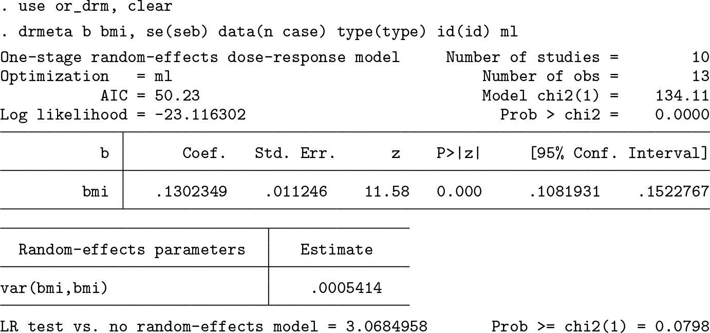
Because a constant change in age-adjusted mortality odds throughout the BMI range can be unrealistic, we next allowed a curvilinear relationship to be detected by using a restricted cubic spline function (M_s ) with three knots at fixed percentiles (10th, 50th, 90th) of the BMI distribution.

The strong reduction in AIC from 50 to -4 and the large value of the Wald-type statistic (H ₀ : β ₂ = 0, z = 7.71, p-value < 0.001) indicate a departure from a simpler trend. A visualization of the summary dose–response relationship based on the spline function and the true summary dose–response mechanism is presented in figure 4. The predicted dose–response relationship between BMI and age-adjusted mortality odds appear to be J shaped with a minimum at around 23.5–24 kg/m², which is not far from what the meta-analysts can expect based on the true dose–response mechanism underlying the population of studies.

Figure 4.

Estimated summary dose–response relationship (solid line) with 95% CIs (short-dashed lines) based on 10 tables of empirical estimates. Data were fit with a weighted mixed-effects model using restricted cubic splines for BMI with three knots located at percentiles (10th, 50th, 90th) of its distribution. The true summary age-adjusted dose–response mechanism (long-dashed line), e^{−2.3(x−24)+0.05(x²−24²)}, is shown for comparison. The value of 24 kg/m² served as the referent.

4.3 Tables of adjusted hazard ratios

Let’s now consider tables of summarized data from 30 hypothetical prospective cohort studies investigating the association between baseline brisk walking, measured in hours/week, and time until death, or end of follow-up (10 years), whichever came first. Age is inversely associated with brisk walking and positively associated with higher mortality rates independently of brisk walking levels. Furthermore, the true summary age-adjusted mortality hazard ratio is decreasing with higher walking levels with a threshold effect at two hours per week; that is e⁻ ⁰ ^. ⁵ ⁽ ^x ⁻ ² ⁾ ⁺⁰ ^. ⁵ ⁽ ^x> ² ⁾⁽ ^x ⁻ ² ⁾. Principal investigators categorized brisk walking into 2/4 quantiles. Age-adjusted mortality hazard ratios comparing brisk walking categories were estimated using a Cox regression model. Each set of empirical estimates arises from a random-effects data-generating mechanism.

The scatterplot of the estimates shown in figure 5 may suggest an overall inverse association between brisk walking and age-adjusted mortality rates. The threshold effect at two hours per week, however, can be hardly guessed in figure 5. There are not even empirical estimates between 1.5 and 2.4 hours per week, exactly in the range where the leveling off is occurring.

Figure 5.

Graph of the study-specific estimated age-adjusted mortality hazard ratios (95% CIs, capped spikes) according to walking levels arising from 30 studies of different sizes. The dark-gray symbols indicate the study-specific reference values. Marker size is inversely related to its variance. The shaded area is the distribution of the dose in the population.

In this example, we directly specify the piecewise linear spline model (M_p ) with a knot at two hours per week to dedicate some attention to useful postestimation commands such as lincom and drmeta‘s predict.

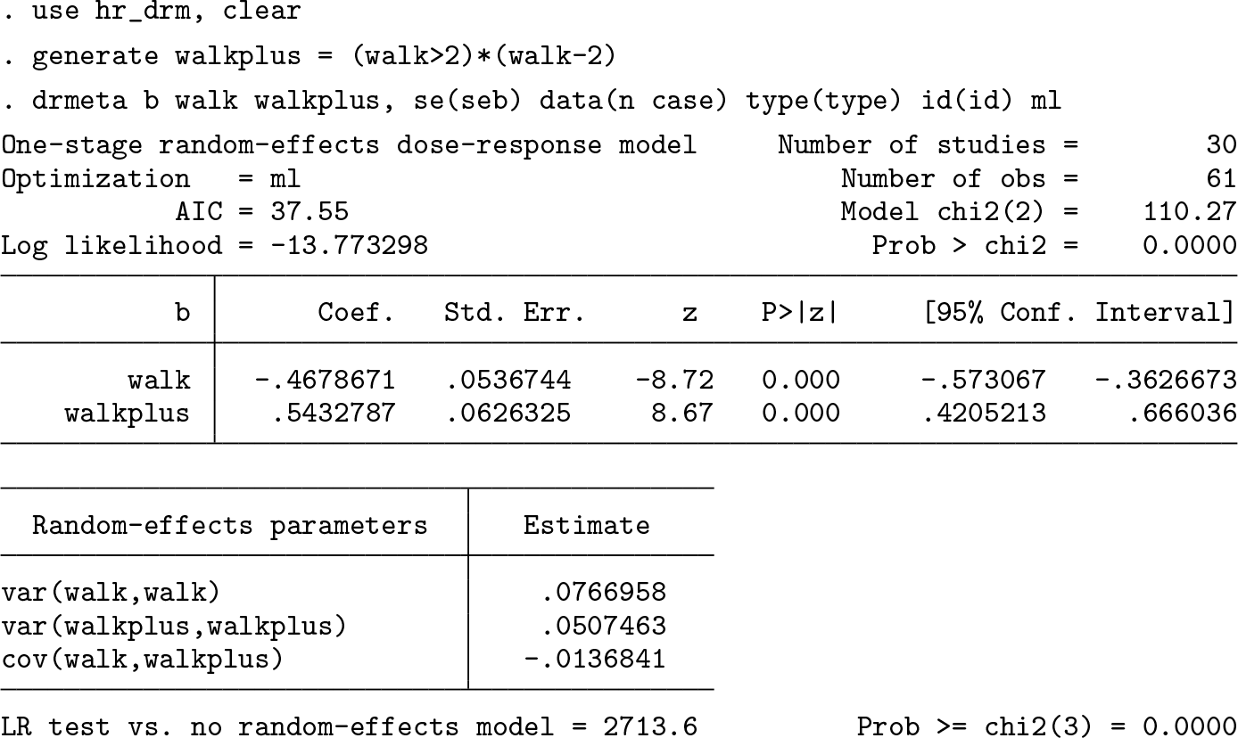
Below 2 hours per week, every increment of 30 minutes per week in brisk walking is estimated to reduce the age-adjusted mortality rate by 21% (HR = e⁻ ⁰ ^. ⁴⁷ ⁽ ¹ ^/ ² ⁾ = 0.79; 95% CI = e⁻ ⁰ ^. ⁴⁷ ⁽ ¹ ^/ ² ^)± ¹ ^. ⁹⁶ ⁽ ⁰ ^. ⁰⁵⁴ ⁾⁽ ¹ ^/ ² ⁾ = [0.75, 0.83]). Above 2 hours per week, every increment of 30 minutes per week in brisk walking is estimated to increase, on average, the age-adjusted mortality rate by 4% [HR = e ⁽⁻ ⁰ ^. ⁴⁷⁺⁰ ^. ⁵⁴ ⁾⁽ ¹ ^/ ² ⁾ = 1.04]. Statistical inference for a combination of parameters and data, such as e ^(β1⁺ ^β 2⁾⁽ ¹ ^/ ² ⁾, can be easily obtained with the lincom postestimation command.

One could be interested in age-adjusted hazard ratios associated with specific levels of brisk walking. For example, those persons who rarely engage in brisk walking (0 hours per week) are expected to have, in an average study, a 2.5-fold increase (95% CI: [2.1, 3.1]) in age-adjusted mortality relative to 2 hours per week.

Various types of predicted values can be obtained after drmeta with the predict postestimation command. Note that in our context, the predicted values of a mixedeffects model with no intercept are changes in predicted responses relative to the studyspecific referent. At the study level, the drmeta_gof command helps visualization of observed and predicted data.

Overlaying predicted summary and study-specific dose–response relationships can help one to appreciate the central tendency and variation across studies. This is achieved by adding estimated regression coefficients, e(b), with the contributions based on the realizations of the random-effects e(blup # ) for the generic study number # and then plotting using a common reference value across all the studies. This information is available right after the drmeta command in the form of returned matrices or via the predict command.

For example, study 20, as compared with the average study, is compatible with a stronger (−0.9 > −0.5) inverse linear relationship below 2 hours per week and stronger, because (−0.9 + 0.4) > (−0.5 + 0.5), inverse linear relationship above 2 hours per week.

The 30 study-specific dose–response relationships can be easily plotted using the blup option of the drmeta_graph command (figure 7). Under a random-effects datagenerating mechanism underlying the studies and tables fit using a weighted mixed-effects model, the meta-analyst can expect approximately an equal spread of study-specific dose–response relationships below and above the average trend. As an example, consider brisk walking levels above 2 hours per week, where about 50% of the studies show an increasing trend and the other 50% of the studies show a decreasing trend. This is not a surprise given the random variation across studies with a true summary age-adjusted hazard ratio equal to 1, that is, a leveling off at 2 hours per week.

Note that the variation of the study-specific dose–response relationships (figure 6) greatly, and correctly, exceeds the uncertainty of the average dose–response response relationship (figure 7). For example, returning to the age-adjusted hazard ratio of 0 versus 2 hours per week (just draw a vertical line at 0), there are two studies compatible with no association (HR ≈ 1) and one study compatible with a very strong positive association (HR = 8). The majority of the studies (28/30 = 0.93) have age-adjusted mortality hazard ratios above 1 when comparing 0 versus 2 hours per week of brisk walking. Considering the variance of the random effects associated with the slope before 2 hours per week, the meta-analyst can expect the middle 95% of the studies to have an age-adjusted mortality hazard ratio comparing 0 versus 2 hours per week between 0.9 and 8; $e^{- 0.47 (0 - 2) \pm 1.96 \sqrt{0.077 {(0 - 2)}^{2}}}$ .

Figure 6.

Estimated summary dose–response relationship (solid line) with 95% CIs (short-dashed lines) based on 30 tables of empirical estimates. Data were fit with a weighted mixed-effects model with piecewise linear splines for brisk walking with one knot located at 2 hours per week. The true summary age-adjusted dose–response mechanism (long-dashed line), e^{−0.5(x−2)+0.5(x>2)(x−2)}, is shown for comparison. The value of 2 hours/week served as the referent.

Figure 7.

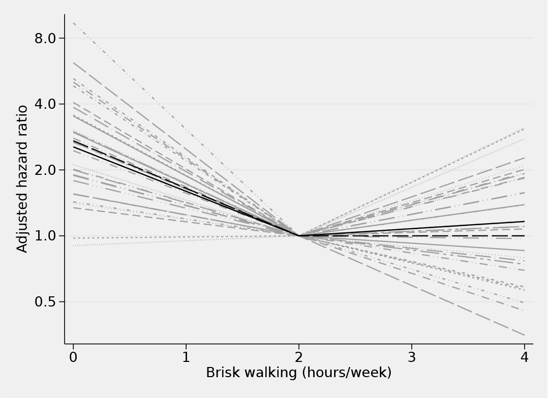
Study-specific dose–response relationships (light gray), summary dose– response relationship (black) based on 30 tables of empirical estimates. Data were fit with a weighted mixed-effects model with piecewise linear splines for brisk walking with one knot located at 2 hours per week. The true summary age-adjusted dose–response mechanism (long-dashed line), e^{−0.5(x−2)+0.5(x>2)(x−2)}, is shown for comparison. The value of 2 hours/week served as the referent.

5 Conclusion

In this article, I described the main features of weighted mixed-effects models suitable for statistical inference on dose–response relationships based on tables of empirical estimates. It can be applied to a variety of research fields where additive and multiplicative measures of association for quantitative predictors are consistently summarized in tabular forms. Tables of empirical estimates can arise from either experimental or observational study designs. Different types of dose transformations can be specified according to the research questions the meta-analyst is willing to ask in light of the data. Although the major focus of inference is usually the average dose–response relationship in a population of studies, mixed models allow examination of the spread of the functional relations across studies.

The drmeta command is illustrated using three hypothetical yet realistic examples that can be encountered in health-related sciences. These examples highlighted the importance of using an appropriate statistical model to move beyond descriptive statistics of empirical estimates and capture the main characteristics of the dose–response datagenerating process. Scatterplots of the empirical estimates are generally not sufficient to acquire some knowledge about the central tendency and spread of dose–response relationships across studies.

Regression splines of a quantitative predictor, such as piecewise constant, linear, and cubic, are flexible tools that can answer a variety of questions. Spline functions are not the only modeling strategy. Applications of the drmeta command are not limited to the use of spline functions; the user can specify other basis functions for the dose. The meta-analyst, however, should keep in mind that the number of parameters to be estimated grows rapidly with the number of dose transformations. If the number of parameters is too large relative to the available data, the estimation procedure will take longer and may fail to converge. In our examples, we intentionally used a maximum of two regression coefficients, making a total of five parameters to be estimated. Information criteria, such as the AIC based on ML, can be used to choose between alternative models.

Although random-effects models are routinely used in quantitative reviews of dose– response data, it is quite rare to see any use of the estimated random effects in applied research. Furthermore, plotting curvilinear relationships is difficult with only few data points available within each study. The drmeta_graph postestimation command has been developed to facilitate the visualization and comparison of predicted average and study-specific dose–response relationships using a common reference dose.

The major challenge for the meta-analyst is to understand that modeling changes in expected responses is not the same as modeling expected responses. Changes in expected responses are themselves the results of a modeling choice by the principal investigator in any given study. The task of using the results of a piecewise constant dose–response function, just another way of calling categorization of the dose, to inform the specification of another dose–response function is unlikely to be straightforward. Although a statistical package can facilitate a variety of calculations and prevent possible mistakes, anyone interested in using the drmeta command for scientific inference is encouraged to use subject-matter knowledge in model specification and to acquire some familiarity with basic statistical principles.

6 Programs and supplemental materials

Supplemental Material, sj-zip-1-stj-10.1177_1536867X211025798 - Weighted mixed-effects dose–response models for tables of correlated contrasts

Supplemental Material, sj-zip-1-stj-10.1177_1536867X211025798 for Weighted mixed-effects dose–response models for tables of correlated contrasts by Nicola Orsini in The Stata Journal

Footnotes

6 Programs and supplemental materials

To install a snapshot of the corresponding software files as they existed at the time of publication of this article, type

References

Berrington

Cox

D. R.

. 2003. Generalized least squares for the synthesis of correlated information. Biostatistics 4: 423–431. https://doi.org/10.1093/biostatistics/4.3.423.

Crippa

Discacciati

Bottai

Spiegelman

, and Orsini

. 2019. One-stage dose–response meta-analysis for aggregated data. Statistical Methods in Medical Research 28: 1579–1596. https://doi.org/10.1177/0962280218773122.

Crippa

Orsini

. 2016. Dose-response meta-analysis of differences in means. BMC Medical Research Methodology 16: 91. https://doi.org/10.1186/s12874-016-0189-0.

Discacciati

Crippa

, and Orsini

. 2017. Goodness of fit tools for dose–response meta-analysis of binary outcomes. Research Synthesis Methods 8: 149–160. https://doi.org/10.1002/jrsm.1194.

Greenland

Longnecker

M. P.

. 1992. Methods for trend estimation from summarized dose–reponse data, with applications to meta-analysis. American Journal of Epidemiology 135: 1301–1309. https://doi.org/10.1093/oxfordjournals.aje.a116237.

Hamling

Lee

Weitkunat

, and Ambühl

. 2008. Facilitating meta-analyses by deriving relative effect and precision estimates for alternative comparisons from a set of estimates presented by exposure level or disease category. Statistics in Medicine 27: 954–970. https://doi.org/10.1002/sim.3013.

Harrell

F. E.

Jr.

2001. Regression Modeling Strategies: With Applications to Linear Models, Logistic Regression, and Survival Analysis. New York: Springer.

Jackson

Riley

, and White

I. R.

. 2011. Multivariate meta-analysis: Potential and promise. Statistics in Medicine 30: 2481–2498. https://doi.org/10.1002/sim.4172.

Müller

Scealy

J. L.

, and Welsh

A. H.

. 2013. Model selection in linear mixed models. Statistical Science 28: 135–167. https://doi.org/10.1214/12-STS410.

10.

Orsini

Bellocco

, and Greenland

. 2006. Generalized least squares for trend estimation of summarized dose–response data. Stata Journal 6: 40–57. https://doi.org/10.1177/1536867X0600600103.

11.

Orsini

Greenland

. 2011. A procedure to tabulate and plot results after flexible modeling of a quantitative covariate. Stata Journal 11: 1–29. https://doi.org/10.1177/1536867X1101100101.

12.

Orsini

Wolk

Khudyakov

, and Spiegelman

. 2012. Meta-analysis for linear and nonlinear dose–response relations: Examples, an evaluation of approximations, and software. American Journal of Epidemiology 175: 66–73. https://doi.org/10.1093/aje/kwr265.

13.

Orsini

Spiegelman

. 2020. Meta-analysis of dose–response relationships. In Handbook of Meta-Analysis, ed. Schmid

C. H.

Stijnen

White

, chap. 18, 395–428. New York: Chapman & Hall/CRC. https://doi.org/10.1201/9781315119403.

14.

Sera

Armstrong

Blangiardo

, and Gasparrini

. 2019. An extended mixed-effects framework for meta-analysis. Statistics in Medicine 38: 5429–5444. https://doi.org/10.1002/sim.8362.

15.

White

I. R.

2009. Multivariate random-effects meta-analysis. Stata Journal 9: 40–56. https://doi.org/10.1177/1536867X0900900103.

Supplementary Material

Please find the following supplemental material available below.

For Open Access articles published under a Creative Commons License, all supplemental material carries the same license as the article it is associated with.

For non-Open Access articles published, all supplemental material carries a non-exclusive license, and permission requests for re-use of supplemental material or any part of supplemental material shall be sent directly to the copyright owner as specified in the copyright notice associated with the article.

0.01 MB

0.00 MB