Sage Journals: Discover world-class research

Abstract

How can social and health researchers study complex dynamic systems that function in nonlinear and even chaotic ways? Common methods, such as experiments and equation-based models, may be ill-suited to this task. To address the limitations of existing methods and offer nonparametric tools for characterizing and testing causality in nonlinear dynamic systems, we introduce the edm command in Stata. This command implements three key empirical dynamic modeling (EDM) methods for time series and panel data: 1) simplex projection, which characterizes the dimensionality of a system and the degree to which it appears to function deterministically; 2) S-maps, which quantify the degree of nonlinearity in a system; and 3) convergent cross-mapping, which offers a nonparametric approach to modeling causal effects. We illustrate these methods using simulated data on daily Chicago temperature and crime, showing an effect of temperature on crime but not the reverse. We conclude by discussing how EDM allows checking the assumptions of traditional model-based methods, such as residual autocorrelation tests, and we advocate for EDM because it does not assume linearity, stability, or equilibrium.

Keywords

st0635 edm empirical dynamic model convergent cross-mapping simplex projection S-maps causality manifold equilibrium

1 Introduction

How can researchers study complex dynamic systems that may not fulfill the assumptions of classic methods such as experiments or model-based regressions? Causal identification is a difficult task in many contexts, including when studying complex dynamic systems wherein experiments or model-based regressions may not be available or appropriate. Dealing with the complexity of real-world phenomena requires tools that can characterize and test causality in nonlinear dynamic systems.

One promising method is called empirical dynamic modeling (EDM) (for an introduction, see Chang, Ushio, and Hsieh [2017]). This novel approach from the natural sciences allows 1) characterizing a dynamic system, including its complexity, predictability, and nonlinearity, as well as 2) distinguishing causation from mere correlation, while 3) making minimal assumptions about nonlinearity, stability, and equilibrium (see Sugihara and May [1990], Sugihara [1994], Sugihara et al. [2012]).

To complement approaches that are more classic, including experiments or model-based regressions, in what follows we offer an overview of the conceptual logic of EDM and then describe the new Stata command edm, which allows researchers to study the nonlinear dynamic systems that may underlie observed time series and panel data— consistent with approaches available in the R packages rEDM and multispatialCCM (see Clark [2014], and see Ye et al. [2016], from which we have borrowed with permission figures 1 and 2). We conclude by noting how these tools may be useful for checking assumptions that underlie other approaches to time-series and panel-data modeling, including by examining their residuals for nonlinear autocorrelation with EDM methods.¹

2 Method

The logic of EDM is based on the fact that a dynamic system producing observed time series or panel data can be modeled by reconstructing the states of the underlying system as it evolves over time (Takens 1981). Consider a system that is characterized by D variables over time, such as a national economy that changes along gross domestic product, unemployment, and inflation, or a person characterized by evolving health and well-being states. Over time, the D variables chart a trajectory of system states as they change, as in figure 1 for D = 3 (showing the Lorenz or “butterfly” attractor and a measure of it as x). 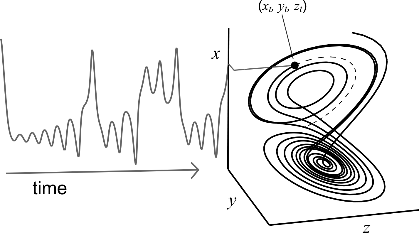As the national economies or individuals evolve, the trajectories of the D variables will trace a D-dimensional “manifold” M in a D-dimensional state space over time. The manifold M represents the system’s trajectory on all D variables as they change over time so that at any time t the system’s state is a single point on M that reflects the D system variables. If the variables are deterministically related (that is, if they cause each other), M will reflect a set of typically unknown differential equations that generate an “attractor” along which the points on M tend to fall. Of course, the attractor may be chaotic rather than a fixed point (equilibrium) or set of points (equilibriums) to which system states tend to converge. The term “dynamic” refers to systems that function in this fashion.

Figure 1.

An example of a dynamic system and its corresponding manifold

If the underlying equations of the attractor manifold M are known, it is elementary to characterize the complexity and nonlinearity of the system; describe its deterministic and stochastic features; and identify causal effects among the D variables. In practice, however, M is unknown and all D variables are not measured. Therefore, M must be reconstructed with an observed variable X from time series (single entity N = 1) or panel data (multiple entities N > 1) with sufficient time length. If X is a projection (that is, measure) of M as in figure 1, Takens’s theorem proves that the deterministic behavior of the entire system can often be reconstructed using merely the lags of X to form an E-dimensional shadow manifold M _X (where D < E ≤ 2D + 1; see Takens [1981] and Sauer, Yorke, and Casdagli [1991]).

This logic also applies to the multivariate case, such as if a stochastic input is also needed to reconstruct a system (Deyle and Sugihara 2011). Figure 2 illustrates this reconstruction process using E = 3 lags of X from figure 1. As figure 2 illustrates, a set of E-length vectors formed by E lags of X are used to reconstruct the original manifold as the shadow manifold M _X (that is, vectors of data on X at each t, t − τ,…, t − (E − 1)τ, where the “time delay” parameter τ > 0).

Figure 2.

An example of manifold reconstruction

Notably, this can also be done using panel data, and in our Stata implementation this case is by default treated using the multispatial method of Clark et al. (2015), wherein E-length vectors of lags on X are taken for each panel separately (so any given point on M _X does not mix data/lags drawn from different panels). Then all the E-length vectors are pooled in analyses, which makes the assumption that all the panels share the same underlying dynamic system while each panel’s longitudinal trajectory contributes to the reconstruction of different sections of the manifold.

Using lags to reconstruct a manifold is a delay embedding or lagged coordinate embedding approach to state-space reconstruction, wherein E-length vectors of lags on X define points on M _X and the quality of the reconstruction is evaluated by the correlation ρ between out-of-sample observed and predicted values (the hallmark of deterministic systems is prediction). The measure ρ reflects the extent to which the underlying system can be recovered by a deterministic manifold reconstructed as M _X . If the original D-dimensional manifold M is properly unfolded as M _X in E-space, then predictive ability ρ will be maximized, and thus ρ across different values of E (that is, different numbers of lags for the embedding) can be used to infer about the underlying system M .

This general approach to reconstructing M with M _X is a useful method for many reasons, including the following: 1) no additional variables beyond X may be needed to capture the dynamics of the entire system; 2) it is unnecessary to control for deterministically coupled unmeasured variables; and 3) no assumptions are made about linearity, stability, or equilibrium (see Glaser, Ye, and Sugihara [2013]).

The edm package takes this approach using three procedures: simplex projection, S-mapping, and convergent cross-mapping (CCM). Simplex projection and S-maps are typically used in an exploratory, diagnostic fashion to characterize the system producing observed time series or panel data (Sugihara and May 1990; Sugihara 1994), whereas CCM is used to evaluate causal effects among variables (Sugihara et al. 2012). We explain each of these in turn, which can be supplemented by the videos noted previously and the brief introductory article by Chang, Ushio, and Hsieh (2017).

2.1 Simplex projection

Simplex projection is a method for investigating the dimension of M and the extent to which a system appears to behave deterministically (Sugihara and May 1990). Even if data appear to be stochastic using typical methods, such as autocorrelation, simplex projection can help show if they are driven by deterministic processes causing chaotic behavior that can masquerade as stochastic. This is done by forming an E-dimensional reconstructed attractor manifold M _X and assessing its characteristics. To reconstruct M as M _X , E lags of X are used to build an E-length vector of data that forms a single point on M _X (that is, an embedding), which is done for each t ≥ E. In our approach, a random 50/50 split of the E-length vectors is used to first form a library of training data to build M _X by default. Note that this is a random split of vectors in the reconstructed manifold rather than the original time-series data. This approach avoids the possible problem of creating additional gaps in the original time-series data. The library of training data therefore becomes a randomly determined set of E-length vectors of lags on X that form points on a reconstructed E-dimensional manifold M _X .

The other half of the data form a “prediction” or test and validation set, which contains E-length target vectors falling somewhere on M _X . Information in the reconstructed manifold M _X can then be used to predict the future of each target. Specifically, for each target x _t in the prediction set, the k = E + 1 nearest neighbors $(x_{t}_{_{1}}, . . ., x_{t_{k}})$ on M _X from the library set are found by Euclidean distances. These k neighbors form a simplex on M _X that is meant to enclose the target x _t in E-space. The simplex of neighbors enclosing the target is then projected into the future $(x_{(t + 1)}_{_{1}}, . . ., x_{(t + 1)}_{_{k}})$ to compute a weighted mean that predicts the future value of the target x _t ₊₁.

A weight w_i associated with each neighbor i is determined by the Euclidean distance of the target to each neighbor and a distance decay parameter θ. Specifically, the weight w_i can be written as

w_{i} = \frac{u_{i}}{\sum_{j = 1}^{k} u_{j}}

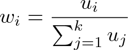
where

u_{i} = \exp (- θ \frac{‖ x_{t} - x_{t_{i}} ‖}{‖ x_{t} - x_{t_{1}} ‖})

and the Euclidean distance measure is denoted ||·||, and x _t ₁ is the nearest neighbor in the manifold (that is, the most similar historical trajectory to the target). When θ = 0, the distances are ignored and all neighbors are weighted equally. As θ increases, the weight of nearby neighbors increases to represent more local states on M _X (that is, more similar historical trajectories on X). By default, θ = 1 to reflect greater weighting of nearer neighbors and, thus, state-dependent evolution on the manifold M . Furthermore, in simplex projection, θ is typically not varied and, instead, is merely fixed to 1 for all analyses. The current version of edm assumes the variables used in the mapping are continuously distributed, but future versions will include updated algorithms to better suit alternative distributions (for example, dichotomous variables).

The quality of predictions is evaluated by the correlation ρ of the future realizations of the targets in the prediction set with the weighted means of the projected simplexes. The mean absolute error (MAE) of the predictions, a measure that focuses more on the absolute gap between observed and predicted data instead of the overall variations like ρ, can also be used as a complement to ρ with the inverse property (that is, higher value indicates poorer prediction) and will range between 0 and 1 when variables are prestandardized (we implement a special z. prefix for this as noted below). When ρ and MAE disagree, some authors have recommended using the lower of the two embedding dimensions E (Glaser et al. 2011), but this often occurs only with noisy data, including shorter time series where ρ may be more sensitive to outliers and thus MAE can be used (Deyle et al. 2013, S1). A familiar term ρ ² may also be used as a type of coefficient of determination (akin to R ²). Whatever the measure of prediction accuracy, by default predictions are out-of-sample because the data used to reconstruct a manifold and make predictions is unshared with the data being predicted (Sugihara and May 1990; Sugihara 1994; Sugihara et al. 2012; Ye et al. 2016).

To simplify prediction, only the first observation in each target vector’s future realization (at t + 1) is used for ρ and MAE (rather than, for example, a multivariate correlation using the entire set of E observations). The resulting ρ and MAE offer insight into how well the reconstructed manifold M _X makes out-of-sample predictions of the future. When the original manifold M is properly unfolded in E-space as M _X , the neighbors of a target point on M _X will provide information about the future of the target (Deyle and Sugihara 2011), meaning ρ > 0 at a given E.

To infer about the underlying system (for example, its dimensionality D), ρ and MAE are evaluated at different values of E, and the functional form of the ρ –E and MAE–E relationships can be used to infer about the extent to which the system appears to be deterministic within the studied time frame (Sugihara and May 1990). Unlike typical regression methods, increasing the dimensionality of a reconstructed manifold by adding additional lags (that is, larger E) will hurt predictions when this adds extraneous information, thus making maximum ρ and minimum MAE useful for choosing E. In low-dimensional systems, adding additional lags by increasing E will add extraneous information that hurts predictions so that ρ is maximized at a moderate E and falls as E increases. In high-dimensional or stochastic systems with autocorrelation, this will not be the case, and ρ may increase with E or appear to approach an asymptote as E increases, which is why the E–ρ and E–MAE relationship is diagnostically useful.

Ideally, a system can be described by fewer than 10 factors (dimensions), such that prediction is maximized when E < 10. In this case, the system may be considered low-dimensional and deterministic to the extent that predictive accuracy is high (for example, ρ > 0.7 or 0.8). In other words, deterministic low-dimensional systems should make good predictions that are maximized when E is relatively small. If prediction continues to improve or improves and then stabilizes as E increases, the system may be tentatively considered stochastic. This may be due to either stochasticity with autocorrelation (for example, an autoregressive process) or high-dimensional determinism that, practically speaking, may be treated as stochastic. To describe such systems parsimoniously, an E may be chosen that does not lose too much information compared with an E that maximizes predictions (for example, by hypothesis tests we describe later), because “it is also important not to overfit the model, and in some cases it may be prudent to choose a smaller embedding dimension that has moderately lower predictive power than a higher dimensional model…We do this both to prevent overfitting the model, and to retain a longer time series” (Clark et al. 2015, s3–s16).

Finally, this general approach can also be made multivariate by including additional observations from different variables in each embedding vector (see Deyle et al. [2013, ^2016a,b], Deyle and Sugihara [2011], and Dixon, Milicich, and Sugihara [1999, 2001]). This is useful when an attractor manifold cannot be fully reconstructed with a single variable, such as with external forces stochastically acting on a system (Stark 1999; Stark et al. 2003). In such a case, simplex projection can be conducted by adding additional variables to the embedding and testing for improved predictive ability—with special considerations for producing similar prediction conditions noted in the work cited here, specifically by using the same number of nearest neighbors when including versus excluding the additional variable in the lagged embedding. Conveniently, if an additional variable participates in an alternative deterministic system, then only a single observation from the alternative system may need to be included in the embedding. If prediction does not improve, then no new information is being provided by the additional variable (as Takens’s theorem implies for coupled deterministic systems). Notably, in any multiple-variable case, standardizing the variables helps ensure an equal weighting for all variables in the embedding (for example, using z scores).

2.2 S-maps

S-maps or “sequential locally weighted global linear maps” are tools for evaluating whether a system evolves in linear or nonlinear ways over time (Sugihara 1994; Hsieh, Anderson, and Sugihara 2008). This is useful because linear stochastic systems such as vector autoregressions (VARs) can be predictable because of autocorrelation, which would appear as a high-dimensional system with ρ > 0 using simplex projection. Therefore, a tool is needed to evaluate whether the system is actually predictable because of deterministic nonlinearity, even if it is high-dimensional. S-maps function as this tool.

A nonlinear system evolves in state-dependent ways, such that its current state influences its trajectory on a manifold M (that is, an unstable process). Conversely, linearity exists if the trajectory on M is invariant with respect to a system’s current state (as assumed in typical VAR and dissipative particle dynamics models). This is evaluated by taking the E chosen from simplex projection and estimating a type of autoregression that varies the weight of nearby observations (in terms of system states rather than time) with a distance decay parameter θ as in simplex projection.

Although we use the term “autoregression”, we are not describing a time-series or panel-data model equation, and instead, the S-map procedure should be interpreted as reconstructing and interrogating a manifold (rather than modeling a series of predictor variables). As with simplex projection, S-maps use a 50/50 split of data into library and prediction sets of E-length embedding vectors by default. The library set represents a reconstructed manifold M _X , and the k nearest neighbors on the manifold in the library set are used to predict the future of each target vector in the prediction set. For S-maps, each of the k neighboring library vectors has E elements that can be thought of as akin to predictors—consider k rows of data with E columns of predictor variables—such that the predictor set includes k neighbors at E occasions t, t − τ, …, t − (E − 1)τ. With a constant term c included by default, this is similar to a local regression with E + 1 predictors and k observations, where E + 1 coefficients are computed to predict each target in the prediction set. Unlike simplex projection (where the number of neighbors k = E + 1), in S-maps, k is often chosen to include the entire library of points on M _X (that is, the entire reconstructed manifold).

Numerically, the predicted value y at point t (from the prediction set) is calculated as

{\hat{y}}_{t} = \sum_{j = 0}^{E} C_{t} (j) x_{t} (j)

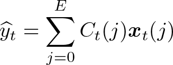
The coefficient vector C _t can be calculated using singular value decomposition in the form B = AC , where B is a k-dimensional vector of the weighted future value for all the neighboring points and A is a weight matrix of the k neighboring points from the library set (that will contain both past and future values from the original time series used to form the randomly determined library used to reconstruct the manifold as M _X ), as well as the constant term (Sugihara 1994). Mathematically, B_i = w_iy_i and A _i = w_i x _i . The weight w_i in S-map is defined as

w_{i} = \exp (- θ \frac{‖ x_{t} - x_{i} ‖}{\frac{1}{k} \sum_{j = 1}^{k} ‖ x_{t} - x_{j} ‖})

When θ = 0 in the weight function, there is no differential weighting of neighbors on M _X , so in the univariate case the S-map is simply an E-order autoregression with a random 50/50 split of training versus prediction data (that is, the mapping is global rather than local). However, as the weight θ increases, predictions become more sensitive to the nonlinear behavior of a system by increasing the weight on nearby neighbors to make predictions. In other words, predictions become more state-dependent by using more information from historical trajectories on M _X that are more similar to targets in a prediction set. If a system evolves in state-dependent ways, more information from nearby neighbors should increase predictive ability.

Again, using ρ and MAE, and looking at the functional form of the ρ–θ and MAE–θ relationships, the nature of a system can be evaluated. If state-dependence is observed in the form of larger ρ and smaller MAE when θ > 0, then EDM tools can be used to model the nonlinear dynamic behavior of the system. If nonlinearity is not observed, EDM tools can still be used to evaluate causal relationships in a nonparametric fashion by using CCM (although CCM may be less efficient than more traditional methods in this case). Here again, S-maps may be useful diagnostically because a linear stochastic system with autocorrelation should show optimal predictions when θ = 0, if for no other reason than increasing local weighting because θ > 0 may increase sensitivity to local noise.

As with simplex projection, S-mapping can also be done in a multivariate fashion (see Deyle et al. [2013], Deyle et al. [2016a], Deyle et al. [2016b], and Dixon, Milicich, and Sugihara [1999, 2001]). Here the interest is in determining whether additional information about a system is contained in other variables because of external forces acting on the system, and tests for improved predictions are possible to evaluate this (with information on how to conduct and interpret such tests described in the work just cited). In the multivariate case, S-maps are more similar to autoregressive-distributed lag or dissipative particle dynamics models, but strictly only when θ = 0. As θ increases, it becomes a more local regression wherein neighbors are identified and predictions increasingly rely on the local information in a reconstructed manifold. Again, standardization can help ensure an equal weighting for the different variables in the model, but remember that the S-map is not a traditional regression model, and instead, is a reconstructed attractor manifold M _X .

2.3 CCM

CCM is a nonparametric method for evaluating causal association among variables, even if they take part in nonlinear dynamic systems (Sugihara et al. 2012). This method is based on the fact that if X is a deterministic driver of Y , or X → Y , then the states of Y must contain information that can contribute to recovering or “cross-mapping” the states of X (Schiff et al. 1996). This method is an extension of simplex projection, such that an attractor manifold M is reconstructed using one variable and this is used to predict a different variable. If variables share an attractor manifold M , then predictions can be made using the reconstructed manifold.

To elaborate, CCM is based on the fact that if variables X and Y participate in the same dynamic system with manifold M , then reconstructed manifolds M _X and M _Y can be mapped to each other. In turn, it is possible to test whether X and Y share information about a common dynamic system, and it is possible to test the extent to which the variables causally influence each other in a directional sense (that is, X → Y and Y → X). This is based on a counterintuitive fact: if X → Y in a causal sense, then historical information about X is contained in Y and thus it is possible to use M _Y to predict X via simplex projection (see Sugihara et al. [2012]), which we symbolize as X| M _Y .

This is counterintuitive because in typical time-series or panel-data methods, causes are used to explain or predict outcomes rather than the reverse. However, in CCM, the outcome Y cross-maps or “xmaps” the causal variable X, with a shadow manifold M _Y predicting X (that is, X ^b = X| M _Y , which heuristically can be read left to right as implying a potential X → Y effect). The outcome is used to predict the causal variable because searching for causes requires starting with an outcome and seeing if its dynamic structure M _Y carries the signature of a cause X (Schiff et al. 1996). Counterintuitively, even if X → Y causality exists (that is, X ^b = X| M _Y works well), if Y does not cause X, then M _X will function poorly when predicting Y because M _X will be a function of variables other than Y (that is, Y ^b = Y | M _X will not work well; Sugihara et al. 2012).

The term “convergent” in CCM describes the criterion by which causality is assessed. This term reflects that if X → Y causality exists then prediction accuracy (for example, a correlation ρ among X and X ^b) will improve as the library size L of points on M _Y increases. Larger libraries improve predictions in this case because they make the manifold M _Y denser, and therefore nearest neighbors become nearer, which improves predictions if causal information exists in the local manifold (Sugihara et al. 2012). However, if X–Y associations are merely statistical, then increasing L should not improve prediction accuracy because denser manifolds will not provide additional predictive information. In sum, if X → Y causality exists, then M _Y will cross-map X in the form of prediction accuracy for X| M _Y , and also, as the number of points L on M _Y increases, prediction accuracy will improve—as tested and graphed via L–ρ (or L–MAE) relationships (see Ye et al. [2015b]).

2.4 Missing data and sample-size considerations

Missing data are currently treated in a way that may aid in a general understanding of EDM. Currently, missing data are by default dealt with using a deletion method, such that a single missing datum causes up to E missing points on a reconstructed manifold M _X . Consider a dataset wherein the t = 10 observation on X is missing. In this case, with E = 3, the embedding vectors at times 8, 9, and 10 will all contain the missing datum (for example, when t = 8, the missing datum takes on the last element in the embedding vector; when t = 10, the missing datum takes on the first element in the embedding vector). Deletion of all E = 3 embedding vectors (that is, points on M _X ) is done because finding nearest neighbors and estimating S-map coefficients requires information in all three dimensions.

Thus, because the manifold exists in E dimensions, any points on the manifold that would include a missing datum cannot be used for computations. Therefore, similar to time-series and panel-data models with lagged regressors wherein the lag order dictates the amount of information lost in the regression, current EDM implementations lose information as a function of E and, of course, the missing-data patterns. Optimally, missing-data rates are low and missing data are missing adjacently in time rather than spread throughout a dataset.

In cases where significant missing values are present, appropriate imputations could help the reconstruction of the manifold as shown in van Dijk et al. (2018). However, we caution the reader to carefully consider typical multiple-imputation or interpolation methods for missing data. The problem with imputation is that typical methods are not sensitive to the nonlinear dynamics that EDM is meant to allow studying. When linear associations are assumed or parametric nonlinear approaches are used, then this can obscure a dynamic signal. The study of how to impute missing values in nonlinear dynamic systems is beyond the scope of our article, but the reader should know that it is not trivial and we are considering various options.²

Many readers may next be considering required sample sizes for EDM analysis. There is no simple cutoff in terms of sample size, but one assumption for EDM is that a dynamic system of interest has been observed across a relevant range of its states over time, by which we mean it has evolved through relevant regions of its state space over time. Preferably, the system will have been observed evolving through these locations more than once to help in the process of determining its proper dimensionality during simplex projection and maximizing predictability in CCM (see Sugihara et al. [2012] and Ye et al. [2015b]). For example, if a system tends to dynamically fluctuate over a 10-year period in terms of some substantive phenomena of interest, then measuring the system over at least a period of 10 years and preferably 20 with adequate resolution would be needed to capture its dynamic behavior patterns—this can be understood as a typical concern about generalizability when considering sampling issues. When describing the edm command options in the following section, we note that using the full dataset for manifold reconstruction and predictions (rather than a 50/50 split) may be useful for smaller datasets.

3 Syntax

The edm command implements a series of tools that can be used for EDM in Stata. The core algorithm is written in Mata to achieve reasonable execution speed—although due to nearest-neighbor search and distance computations, the program slows down considerably as sample sizes increase beyond a few thousand. The command keyword, edm, should be immediately followed by one of the main subcommands explore or xmap. A dataset must be declared as time series or panel data by the tsset or xtset command prior to using the edm command, and time-series operators including l., f., d., and s. can be used (the last for seasonal-differencing). Standardizing variables used in the main analysis can also be done with the prefix z., which uses z scores for analysis instead of the original variable. When combined with time-series operators such as first-differencing with z.d. (the z. must appear first), the z scores are computed after the first-differencing.

The first main subcommand, explore, follows the syntax below and supports one main variable for exploration using simplex projection or S-mapping. In the case of multivariate embedding, the option extraembed(), or simply extra(), can be used. A multivariate embedding is constructed as follows: the main variable forms an E-dimensional lagged embedding starting at t, and a single observation at t from the additional variables are added as the last elements in the embedding (in S-maps this will mean the last columns of data in the regression will belong to the additional variables).

edm explore varlist [ if ] [ , e( numlist ) tau( integer ) theta( numlist ) k( integer )

algorithm( string ) replicate( integer ) dot( integer ) tp( integer ) seed( integer )

predict( varname ) copredict( varname ) copredictvar( varlist )

crossfold( integer ) ci( integer ) extraembed( varlist ) allowmissing

missingdistance( real ) dt dtweight( real ) dtsave( varname ) details full

force reportrawe ]

The second main subcommand, xmap, performs CCM and follows the syntax below. It requires a varlist of two variables to follow immediately after xmap. It shares many of the same options with the explore subcommand, although there are some differences given the different purpose of the analysis.

edm xmap varlist [ if ] [ , e( integer ) tau( integer ) theta( real ) library( numlist )

k( integer ) algorithm( string ) replicate( integer ) dot( integer ) tp( integer )

direction( string ) seed( integer ) predict( varname ) copredict( varname )

copredictvar( varlist ) ci( integer ) extraembed( varlist ) allowmissing

missingdistance( real ) dt dtweight( real ) dtsave( varname ) oneway details

force savesmap( string ) ]

Both main subcommands support the if qualifier. The options are detailed in the next section, and additional options will be introduced while the package is under active development.

Additionally, the edm command has the utility subcommands version and update, with syntax as follows:

edm version

edm update [ , develop replace ]

edm version reports the current version number.

edm update allows the user to update the ado-file. The update subcommand supports the options develop and replace. develop updates the command to its latest development version. The development version usually contains more features but may be less tested compared with the version available through the Statistical Software Components Archive. replace allows the update to override your local ado-files. Together, these allow the user to update the edm program to the latest development version by running edm update, develop replace.

3.1 Options

e( numlist ) specifies in ascending order the number of dimensions E used for the main variable in the manifold reconstruction. If a list of numbers is provided, the command will compute results for all numbers specified. The xmap subcommand only supports a single integer as the option, whereas the explore subcommand supports a numlist. The default is e(2), but in theory E can range from 2 to almost half of the total sample size. The actual E used in the estimation may be different if additional variables are incorporated. An error message occurs if the specified value is out of range. Missing data will limit the maximum E under the default deletion method.

tau( integer ) allows researchers to specify the time delay, which essentially sorts the data by the multiple τ. This is done by specifying lagged embeddings that take the form t, t − τ,…, t − (E − 1)τ, where the default is tau(1) (that is, typical lags). However, if tau(2) is set, then every other t is used to reconstruct the attractor and make predictions—this does not halve the observed sample size because both odd and even t would be used to construct the set of embedding vectors for analysis. This option is helpful when data are oversampled (that is, spaced too closely in time) and therefore very little new information about a dynamic system is added at each occasion. The tau() setting is also useful if different dynamics occur at different time scales and can be chosen to reflect a researcher’s theory-driven interest in a specific time scale (for example, daily instead of hourly). Researchers can evaluate whether τ > 1 is required by checking for large autocorrelations in the observed data (for example, using Stata’s corrgram command). Of course, such a linear measure of association may not work well in nonlinear systems, and thus researchers can also check performance by examining ρ and MAE at different values of τ.

theta( numlist ) specifies in ascending order the distance weighting parameter for the local neighbors in the manifold. It is used to detect the nonlinearity of the system in the explore subcommand for S-mapping. Of course, as noted above, for simplex projection and CCM, a weight of theta(1) is applied to neighbors based on their distance, which is reflected in the default of theta(1). However, this can be altered even for simplex projection or CCM (two cases that we do not cover here). Particularly, values for S-mapping to test for improved predictions as they become more local may include the following option: theta(0 .00001 .0001 .001 .005 .01 .05 .1 .5 1 1.5 2 3 4 6 8 10).

library( numlist ) is only available with the xmap subcommand. library() specifies in ascending order the total library size L used for the manifold reconstruction. Varying the library size is used to estimate the convergence property of the cross-mapping, with a minimum value L _min = E + 2 and the maximum equal to the total number of observations minus sufficient lags (for example, in the time-series case without missing data, this is L _max = T + 1 − E). An error message is given if the L value is beyond the allowed range. To assess the rate of convergence (that is, the rate at which ρ increases as L grows), the full range of library sizes at small values of L can be used, such as if E = 2 and T = 100, with the setting then perhaps being library(4(1)25 30(5)50 54(15)99).

k( integer ) specifies the number of neighbors used for prediction. When set to k(1), only the nearest neighbor is used. As k increases, the next-closest nearest neighbors are included for making predictions. In the case of k(0), the default value, the number of neighbors used is calculated automatically (typically as k = E + 1 to form a simplex around a target). When k < 0 (for example, k(-1)), all possible points in the prediction set are used (that is, all points in the library are used to reconstruct the manifold and predict target vectors). This latter setting is useful and typically recommended for S-mapping because it allows all points in the library to be used for predictions with the weightings in theta(). However, with large datasets this may be computationally burdensome, and therefore k(100) or perhaps k(500) may be preferred if T or NT is large.

algorithm( string ) specifies the algorithm used for prediction. By default, simplex projection (a locally weighted average) is used. Valid options include simplex and smap, the latter of which is a sequential locally weighted global linear mapping (S-map). With the xmap subcommand, where two variables predict each other, algorithm(smap) invokes something analogous to a distributed lag model with E+1 predictors (including a constant term c) and, thus, E +1 locally weighted coefficients for each predicted observation/target vector—because each predicted observation has its own type of regression done with k neighbors as rows and E + 1 coefficients as columns. As noted below, special options are available to save these coefficients for postprocessing, but again, it is not actually a regression model and instead should be seen as a manifold.

replicate( integer ) specifies the number of repeats for estimation. The explore subcommand uses a random 50/50 split for simplex projection and S-maps, whereas the xmap subcommand selects the observations randomly for library construction if the size of the library L is smaller than the size of all available observations. In these cases, results may be different in each run because the embedding vectors (that is, the E-dimensional points) used to reconstruct a manifold are chosen at random. The replicate() option takes advantage of this to allow repeating the randomization process and calculating results each time. This is akin to a nonparametric bootstrap without replacement and is commonly used for inference using confidence intervals (CIs) in EDM (Tsonis et al. 2015; van Nes et al. 2015; Ye et al. 2015b). When, for example, replicate(50) is specified, mean values and the standard deviations of the results are reported across the 50 runs by default. As we note below, it is possible to save all estimates for postprocessing using typical Stata commands, such as allowing the graphing of results with the svmat command or finding percentile-based measures with the pctile command.

dot( integer ) controls the appearance of the progress bar when the replicate() or crossfold() option is specified. The default is dot(1) or one dot for each completed cross-mapping estimation. dot(0) removes the progress bar.

tp( integer ) adjusts the default forward-prediction period. By default, the explore mode uses tp(1) and the xmap mode uses tp(0). To show results for predictions made two periods into the future, for example, use tp(2).

direction( string ) is only available with the xmap subcommand. direction() allows users to control whether the cross-mapping is calculated bidirectionally or unidirectionally (which reduces computation times if bidirectional mappings are not required). Valid options include oneway and both, the latter of which is the default and computes both possible cross-mappings. When oneway is chosen, the first variable listed after the xmap subcommand is treated as the potential dependent variable, so edm xmap x y, direction(oneway) produces the cross-mapping Y | M _X , which pertains to a Y → X effect. This is consistent with the beta1 coefficients from the savesmap(beta) option. On this point, the direction(oneway) option may be especially useful when an initial edm xmap x y procedure shows convergence only for a cross-mapping Y | M _X , which pertains to a Y → X effect. To save time with large datasets, any follow-up analyses with the algorithm(smap) option can then be conducted with edm xmap x y, algorithm(smap) savesmap(beta) direction(oneway). To make this easier, there is also a simplified oneway option that implies direction(oneway).

seed( integer ) specifies the random-number seed for reproducibility.

predict( varname ) allows saving the internal predicted values as a variable, which could be useful for plotting and diagnostics as well as forecasting.

copredict( varname ) allows you to save the coprediction result as a variable. You must specify the copredictvar( varlist ) option for this to work.

copredictvar( varlist ) is used together with the copredict() option and specifies the variables used for coprediction. The number of variables must match the main variables specified.

crossfold( integer ) asks the program to run a cross-fold validation of the predicted variables. crossfold(5) indicates a 5-fold cross validation. Note that this cannot be used together with replicate(). This option is only available with the explore subcommand.

ci( integer ) reports the CI for the mean of the estimates (MAE and ρ), as well as the percentiles of their distribution when used with replicate() or crossfold(). The first row of output labeled Est. mean CI reports the estimated CI of the mean ρ, assuming that ρ has a normal distribution—estimated as the corrected sample standard deviation (with N − 1 in the denominator) divided by the square root of the number of replications. The reported range can be used to compare mean ρ across different (hyper) parameter values (for example, different E, θ, or L) using the same datasets as if the sample were the entire population (such that uncertainty is reduced to 0 when the number of replications → ∞). These intervals can be used to test which (hyper) parameter values best describe a sample, as might be typical when using cross-fold validation methods. The row labeled with Pc (Est.) follows the same normality assumption and reports the estimated percentile values based on the corrected sample standard deviation of the replicated estimates. The row labeled Pc (Obs.) reports the actual observed percentile values from the replicated estimates. In both Pc (Est.) and Pc (Obs.), the percentile values offer alternative metrics for comparisons across distributions, which would be more useful for testing typical hypotheses about population differences in estimates across different (hyper) parameter values (for example, different E, θ, or L), such as testing whether a dynamic system appears to be nonlinear in a population (that is, testing whether ρ is maximized when θ > 0).

The number specified within the ci() bracket determines the confidence level and the locations of the percentile cutoffs. For example, ci(90) instructs edm to return 90% CIs as well as the cutoff values for the 5th and 95th percentile values (because ρ and MAE values cannot or are not expected to take on negative values, we typically prefer one-tailed hypothesis tests and therefore would use ci(90) to get a one-tailed 95% interval). These estimated ranges are also included in the e() return list as a series of scalars with names starting with ub for upper bound and lb for lower bound values of the CIs. These return values can be used for further postprocessing.

extraembed( varlist ) allows incorporating additional variables in the embedding (that is, a multivariate embedding), for example, extraembed(z l.z) for the variable z and its first lag l.z. The special prefix for standardization, z., also works here.

allowmissing allows observations with missing values to be used in the manifold. Vectors with at least one nonmissing value will be used in the manifold construction. When allowmissing is specified, distance computations are adapted to allow missing values.

missingdistance( real ) allows users to specify the assumed distance between missing values and any values (including missing) when estimating the Euclidean distance of the vector. This enables computations with missing values. missingdistance() implies allowmissing. By default, the distance is set to the expected distance of two random draws in a normal distribution, which equals $2 / \sqrt{π}$ ×standard deviation of the mapping variable.

dt allows automatic inclusion of timestamp-differencing in the embedding. Generally, there will be E − 1 dt variables included for an embedding with E dimensions. By default, the weights used for these additional variables equal the standard deviation of the main mapping variable divided by the standard deviation of the time difference. This can be overridden by the dtweight() option. The dt option will be ignored when running with data with no sampling variation in the time lags.

dtweight( real ) specifies the weight used for the timestamp-differencing variable.

dtsave( varname ) allows users to save the internally generated timestamp-differencing variable.

oneway is equivalent to the direction(oneway) option and is also available only with the xmap subcommand.

details asks the program to report the results for all replications instead of a summary table with mean values and standard deviations when the replicate() or crossfold() option is specified. Irrespective of using this option, all results can be saved for postprocessing.

full is available only with the explore subcommand. full asks the program to use all possible observations in the manifold construction instead of the default 50/50 split. This is effectively the same as leave-one-out cross-validation because the observation itself is not used for the prediction. This may be useful with small samples (for example, T < 50), where a random split would result in a manifold with an insufficient number of data points (neighbors) used for calculations when conducting a search for optimal up to roughly 20. Sample-size considerations, however, extend beyond this and include whether data contain runs of repeated values that offer no unique information for prediction. Furthermore, as noted previously, one assumption for EDM is that a system has been observed across a relevant range of locations in its state space over time (and preferably, the system will have evolved through these locations more than once). When in doubt, use the full option to take advantage of all information available in a dataset for manifold reconstruction and prediction.

force asks the program to try to continue even if the required number of unique neighboring observations is not sufficient given the default or user-specified k(), such as when there are many repeated values that must be excluded. This is a common case in past research, where E-length runs of zeros have been excluded by default because they add no unique information (see Deyle et al. [2016a]).

reportrawe is available only with the explore subcommand. reportrawe asks the program to report the number of dimensions constructed from the main variable that is associated with the requested e(). By default, the program reports the actual E used to reconstruct the manifold, which will include any variables used with the extraembed() option.

savesmap( string ) is available only with the xmap subcommand. savesmap() allows S-map coefficients to be stored in variables with a specified prefix. For example, specifying savesmap(beta) will create a set of new variables with the prefix beta, such as beta1_b0_rep1. The specified prefix must not be shared with any variables in the dataset, and the option is valid only if the algorithm(smap) option is also specified.

In the newly created variables, the first number immediately after the prefix is 1 or 2 and indicates which of the two listed variables is treated as the dependent variable in the cross-mapping (that is, it indicates the direction of the mapping). If the command is, for example, edm xmap x y, algorithm(smap) savesmap(beta) k(-1), then variables starting with beta1_ contain coefficients derived from the manifold M _X created using the lags of the first variable x to predict Y , or Y | M _X . This set of variables, therefore, store the coefficients related to x as an outcome rather than a predictor in CCM. Any Y → X effect associated with the beta1 prefix is shown as Y | M _X , because the outcome is used to cross-map the predictor, and thus the reported coefficients will be scaled in the opposite direction of a typical regression (because in CCM, the outcome variable predicts the cause).

Variables starting with beta2_ in the above example store the coefficients (which will be locally weighted) estimated in the other direction, where the second listed variable y is used for the manifold reconstruction M _Y for the mapping X| M _Y , testing the opposite X → Y effect in CCM but with reported S-map coefficients that map to a Y → X regression. This may be unintuitive, but because CCM causation is tested by predicting the causal variable with the outcome, to get more familiar regression coefficients requires reversing CCM’s causal direction to a more typical predictor outcome regression logic. This can be clarified by reverting to the conditional notation, such as X| M _Y , which in CCM implies a left to right X → Y effect, but for the S-map coefficients will be scaled as a locally weighted regression in the opposite direction, Y → X.

Following the beta1 or beta2 is the letter b and a number. The numerical labeling scheme follows the order of the lag for the main variable and then the order of the extra variables introduced in the case of multivariate embedding. b0 is a special case that records the coefficient of the constant term in the regression.

The final term, rep1, indicates that the coefficients are from the first round of replication (if the replicate() option is not used, then there is only one round). Finally, the coefficients are saved to match the observation t in the dataset that is being predicted, which allows plotting each of the E estimated coefficients against time and the values of the variable being predicted. The variables are also automatically labeled for clarity.

4 Output and stored results

Typical output from using the explore subcommand is shown below.

The output includes the selected range of system dimensions E and θ values, and it reports the corresponding mapping/prediction accuracies in the form of ρ (correlation coefficient) and MAE. By prestandardizing the variables used, MAE can be understood as the conceptual inverse of ρ (that is, 1−MAE), and these can then be plotted together.

Typical output from using the xmap subcommand is shown below.

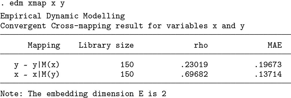
The output shows a table listing the direction of the mapping. The notation x ˜ x|M(y) indicates a comparison between the observed x values and the predicted x values using a manifold reconstructed from y. Recall that because of the counterintuitive nature of CCM, a prediction X| M _Y allows testing for a causal effect in an X → Y fashion. ρ and MAE are reported. By default, the maximum library size is used unless the library() option is specified. Users should expect significant computation time when a large library is used.

In addition to the table output, the edm command also stores the results in e() as matrices for postprocessing. Notably, return matrices include the following:

e(explore_result) stores the ρ and MAE values for each combination of the parameters in the exploration mode.

e(xmap_1) and e(xmap_2) store the ρ and MAE values in the cross-mapping results, with one matrix per direction of potential causality. The suffix of the matrix indicates the direction of the implied causality. In the case of e(xmap_1), it stores the result where the observed value of the first variable was considered as the dependent variable; if the command edm xmap x y is used, this will be the mapping y ˜ y|M(x) pertaining to a Y → X effect (that is, the first listed variable is caused by the second). Alternatively, the matrix e(xmap_2) contains the results associated with the mapping x ˜ x|M(y), which would pertain to an X → Y effect (that is, the second listed variable is caused by the first). The numbering in the return matrix is consistent with the saved coefficients in the savesmap() option, as well as the intent of the direction(oneway) option, where the first listed variable is treated as an outcome of the second (as in regress x y).

5 Examples

5.1 Creating a dynamic system

The logistic map has often been used to demonstrate a nonlinear dynamic system, displaying regular periodic behavior as well as deterministic chaos (May 1976). This particular system has been widely cited in EDM literature (see Perretti, Munch, and Sugihara [2013], Ye and Sugihara [2016], and Mønster et al. [2017]). Here we create an arbitrary dynamic system with two logistic maps coupled through linear coefficients to illustrate the use of the edm command. Our focus is mostly on the statistical properties of the data and the EDM results for a model:

\begin{array}{l} x_{t} = x_{t} {_{-}}_{1} {3.79 (1 - x_{t} {_{-}}_{1}) - 0.00 y_{t} {_{-}}_{1}} \\ y_{t} = y_{t}_{- 1} {3.79 (1 - y_{t}_{- 1}) - 0.20 x_{t}_{- 1}} \end{array}

A logistic map is well known to exhibit chaotic patterns with a specific combination of parameters (Jackson and Hübler 1990). The values in the equations were chosen to exploit this property, creating a dynamic system. The two variables x and y both depend on their own past values and are coupled with each other through the last term of the equation. In this case, x is set to be determined by its own past values only, while y is determined by past values of both y and x.

Figure 3 plots the values for x and y over time, when x ₁ and y ₁ are set to 0.2 and 0.3, respectively. Observations with a t smaller than 300 were burned to allow the dynamics to mature.³ The pairwise correlation coefficient between x and y is 0.15, and it is not significant at the 0.05 level, giving the appearance of two unrelated variables. Indeed, the plot from figure 3 shows that the variables could appear positively or negatively correlated depending on the temporal window in which data were collected from the system. This case mimics a potentially common scenario wherein “mirage correlations” can exist in a dataset and, more importantly, causation can be inferred without the presence of a linear correlation (which, using typical linear indices such as correlation coefficients, would be missed).

Figure 3.

Plot of a nonlinear dynamic system

5.2 Exploring the system’s dimensionality

The first step in EDM analysis is to establish the dimensionality of the system, which can be understood as approximating the number of independent variables needed to reconstruct the underlying attractor manifold M that defines the system (Sugihara and May 1990; Sugihara et al. 2012). This is done by simplex projection with the explore subcommand, using the range of dimensions specified in the e() option.

Using the explore subcommand, the data are randomly split into two halves, wherein one half is used as the library (or training) dataset to construct the shadow manifold M _X , and the other half is the prediction (or test) dataset used to evaluate the out-of-sample predictive ability of the projections on M _X . The optimal E is often selected based on the highest ρ or lowest MAE between the predicted and the observed values (while also attempting to keep the model somewhat parsimonious). These two measures generally agree, but if they do not, then the one indicating the lowest embedding dimension E may be used (Glaser et al. 2011). In the case of small samples, MAE may be preferred because it is less sensitive to outliers (Deyle et al. 2013).

In this example, we explore all dimensions between 2 and 10 using simplex projection to identify the optimal E.⁴ Because the library set is randomly selected, we replicated the method 50 times through the option replicate(50) to estimate the average performances across the 50 runs. The command and the output are shown below.

The standard deviations are bias-corrected, using N − 1 in the denominator. Note that the reported standard deviation values are summary statistics instead of the standard error of the ρ and MAE estimates. The ci() option can be used to report the estimated CIs for the mean value of ρ derived from multiple replications. The edm command can also be used in combination with the jackknife prefix for additional controls. It is common to select the E value with the highest ρ or lowest MAE, because its reconstructed manifold best matches the observed data (Sugihara et al. 2012; Ye et al. 2015b).

The results show that ρ drops and MAE increases as E increases. This suggests that the optimal E is 2, which is the exact number of independent variables we used to create the dynamic system. The result can also be plotted using the contents of the stored e(explore_result) matrix, as shown in figure 4. Also, hypothesis tests can be performed on ρ and MAE at different values of E by using methods we describe below, which may be useful for selecting E with an interest in maintaining model parsimony (that is, smaller E) as is often done in autoregressions.

Figure 4.

ρ –E plot of variable y

5.3 Nonlinearity detection using S-map

We next evaluate the system for nonlinearity by using S-maps or “sequentially locally weighted global linear maps” (Sugihara 1994; Hsieh, Anderson, and Sugihara 2008). Linearity exists if the trajectory on a manifold M is invariant with respect to a system’s current state, whereas nonlinearity exists if system evolution is state-dependent. This is evaluated by taking the optimal E chosen from simplex projection and fitting a type of regression model that varies the weight of nearby observations (in terms of system states rather than time) with a distance decay parameter θ. Again, however, we emphasize that it should not be interpreted as a typical regression model, but rather as a reconstructed manifold.

When θ = 0 in the option theta(0), there is no differential weighting of neighbors on M _X , so the S-map reduces to a type of autoregressive model with a random 50/50 split of library versus prediction data. However, as θ increases, predictions become more sensitive to the nonlinear behavior of a system by drawing more heavily on nearby observations to make predictions. In other words, predictions become more state-dependent. Again using ρ and MAE and forming ρ–θ and MAE–θ plots, the nonlinearity of the system can be evaluated. If nonlinearity or state-dependence is observed in the form of larger ρ and smaller MAE when θ > 0, EDM tools are needed to model system behavior. If the system is linear, ρ would not increase as θ goes above zero. In this case, models with linearity assumptions may also be appropriate such as, potentially, autoregressive approaches.

Both the explore and xmap subcommands support S-mapping instead of simplex projection for the local predictions. An example is given below to analyze the nonlinearity of the variable y in the previous example. In this case, we explore possible θ values between 0 and 5 with an increment of 0.01. Additionally, we include all observations for the local prediction by specifying a negative number in the k() option. This allows for more stable results with low E or in low data-density regions of M _Y .

The result from the command above can also be plotted graphically using the return matrix e(explore_result) as shown in figure 5. The increase of ρ as θ increases is consistent with the characteristics of a highly nonlinear system such as the logistic map. As we show below, hypothesis tests of change in ρ or MAE can be done to test for improvements in predictive ability when θ = 0 versus maximum ρ or minimum MAE (that is, a test of Δρ or ΔMAE; Hsieh and Ohman [2006], Glaser, Ye, and Sugihara [2013], Ye et al. [2015a]).

Figure 5.

Nonlinearity diagnosis (ρ–θ plot) of variable y

5.4 Causality detection using CCM

In the earlier steps, the analysis suggests that the optimal E for this example is 2, which is what we expect given the data generation. We now use the xmap subcommand to derive the bivariate (overall) causal effect between the variables x and y using the previously observed E = 2 value. In most cases, we would recommend standardizing variables to put them on the same scale, however, in this hypothetical example it is less relevant.

In CCM, the causal link between variables is evaluated by predicting values of one variable—the potential cause—using the reconstructed manifold of another—the potential outcome—which is based on Sugihara et al. (2012). In essence, this is a kind of two-variable simplex projection wherein the library set is formed using one variable and contemporaneous predictions are made for another variable. Using the predicted versus observed values, ρ and MAE are calculated. It should be noted that bivariate cross-mapping captures the overall causal effect, combining both the direct effect (X → Y ) and the possible indirect effects (X → Z → Y ).⁵

Simplex projection may show that different E values characterize different variables. If this were the case, the E chosen for reconstructing a manifold can be used with the direction(oneway) option to run separate CCM procedures for each variable. Then the causal variable’s E can be used because its signal is being predicted by the outcome. For example, if E = 2 for y but E = 4 for x, the following CCM could be run: edm xmap x y, e(2) direction(oneway) for the Y | M _X or Y → X case; or edm xmap y x, e(4) direction(oneway) for the X| M _Y or X → Y case. Here the manifold reconstructed by the first variable is used to predict the second, so the E from simplex projection applies to the second variable listed.

The xmap subcommand facilitates CCM. An example is as follows:

Without specifying a value for library(), by default the entire dataset is used as the library. In other words, all possible information from one variable is used to make predictions of another. This will often be a useful first step in CCM because it is not always easy to know beforehand what the maximum library size is (for example, in the panel-data case with imbalanced data, etc.), and this value can then be manually added later as the maximum library size when evaluating results across L. Furthermore, if CCM at the maximum L shows no meaningful predictability, then the question of convergence is moot. Specifically, if there is a causal X → Y relationship (that is, X| M _Y ), then we expect meaningful predictions at maximum L and prediction should improve as more data points are used in the library. To assess this, the library() option specifies the range of the library sizes, and the replicate() option allows repeating the estimations to show the impact of random sampling at the lower library lengths. When the specified library size is smaller than the maximum available size, a random subsample is selected for the manifold reconstruction and the replicate() option becomes possible.

The example below estimates ρ at library sizes between 5 and 150, and repeats the process 10 times (taking a random draw to form the manifold 10 times at each library size). Multiple repeats are used to ensure enough point estimates (number of repeats for each step in library size) to clearly identify any trends in predictability ρ as the library size increases, as well as differences in these trends between both directions for the mappings (both x–y and y–x; see figure 6). For the maximum library size, this replication process does not produce different results because all observations are used. Because this maximum library size is the most computationally demanding, with large datasets it may be prudent to separately run the xmap procedure at the maximum library size only once, and then use the replicate() option at small library sizes only to assess uncertainty.

The detailed results are stored in two return matrices, e(xmap_1) and e(xmap_2), which can be converted to variables for easy manipulations using Stata’s svmat command. Recall that e(xmap_1) treats the first-listed variable, x, as the outcome of the second, y (that is, Y | M _X ), and e(xmap_2) treats the second-listed variable, y, as the outcome of the first, x (that is, X| M _Y ). The example below stores the results and plots the ρ –L convergence graph as in figure 6. Each plotted dot represents a point estimate, and there are 10 estimates for each library size as specified by replicate(10). The local polynomial smoothing lines show the general trend of the ρ values as the reconstructed manifold gets denser (that is, as L increases).

Figure 6.

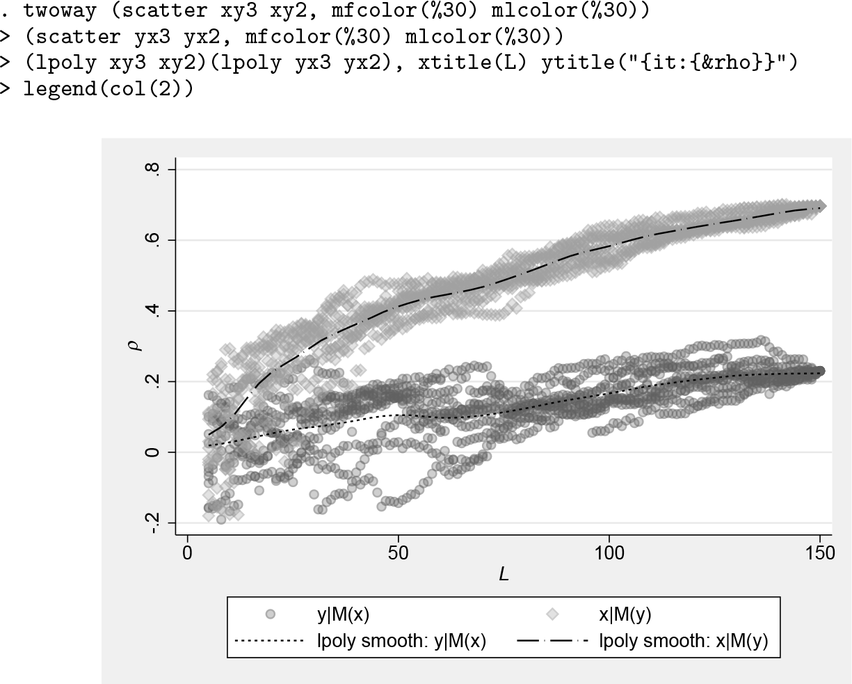
ρ –L convergence diagnosis

The ρ –L diagnosis figure suggests that the predicted x from the manifold constructed from y (that is, x| M _y ) consistently outperforms the reversed pair, suggesting the data series y contains more information about x than the other way around. This indicates that x CCM-causes y (that is, X → Y ), which matches the reality of the model wherein y is caused by x but x is entirely determined by its lagged values rather than y. As we now show, this and other hypotheses can be tested directly in various ways. Also note that the results do not necessarily rule out the possibility of a bidirectional causal relationship, especially when both predictions are similar and at a relatively high level. In such a case, the relative difference in the prediction performances may be used to determine the more dominant causal direction without precluding an inference of bidirectional causality. When prediction performances from both directions are poor,⁶ it is also reasonable to consider the possibility that the variables are causally independent. Alternatively, when predictability is high for both variables but no convergence is observed, then an exogenous third variable may potentially be driving both variables.

5.5 Hypothesis testing with CIs and null distributions

There are three primary ways to test hypotheses about causal effects and dominant causal direction in our edm package that we treat here: jackknifing, multiple replications with the replicate() option (using the ci() option to enable automated reporting of the CI for the mean ρ), and surrogate-data methods that use permutations on t to form null distributions. The first two rely on the random selection of observations to reconstruct a manifold, creating variation in results.

One way to estimate the standard error of the estimates due to the resampling process is with the jackknife prefix, which generates estimates for ρ. A CCM example is as follows:

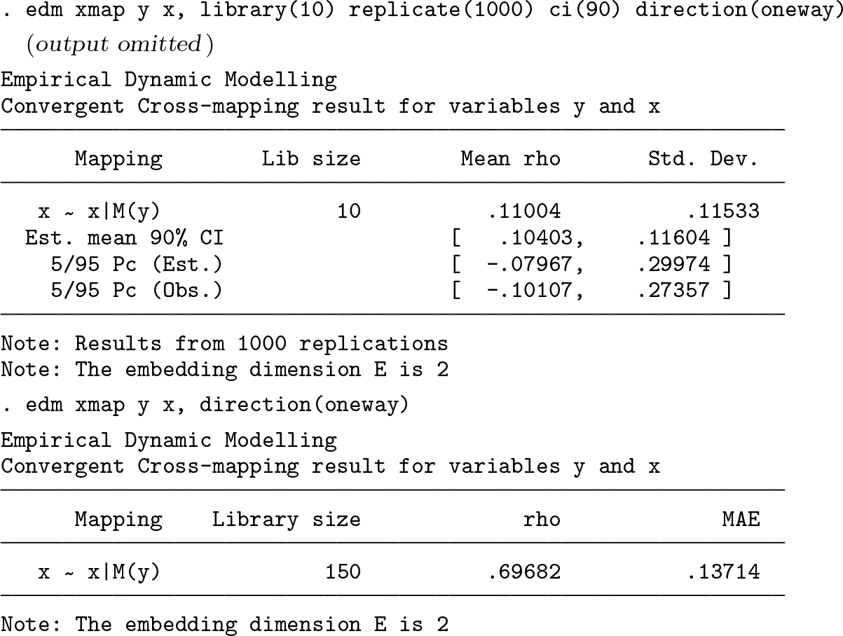
This is particularly useful in CCM because it offers a CI around ρ at the maximum library size, which is arguably the best estimate of ρ in CCM applications. The replicate() option cannot do this because the full dataset is used to construct the library in this case. Jackknifing can also be used for simplex projection and S-maps by using the explore subcommand, but other methods are also available. For the jackknife, users should fix E, L, and τ prior to the jackknife process because the results only contain the last set of estimates in the jackknife mode (that is, common E, L, and τ). However, this method does not evaluate convergence in CCM, which implies an increase in ρ as the library size L increases.

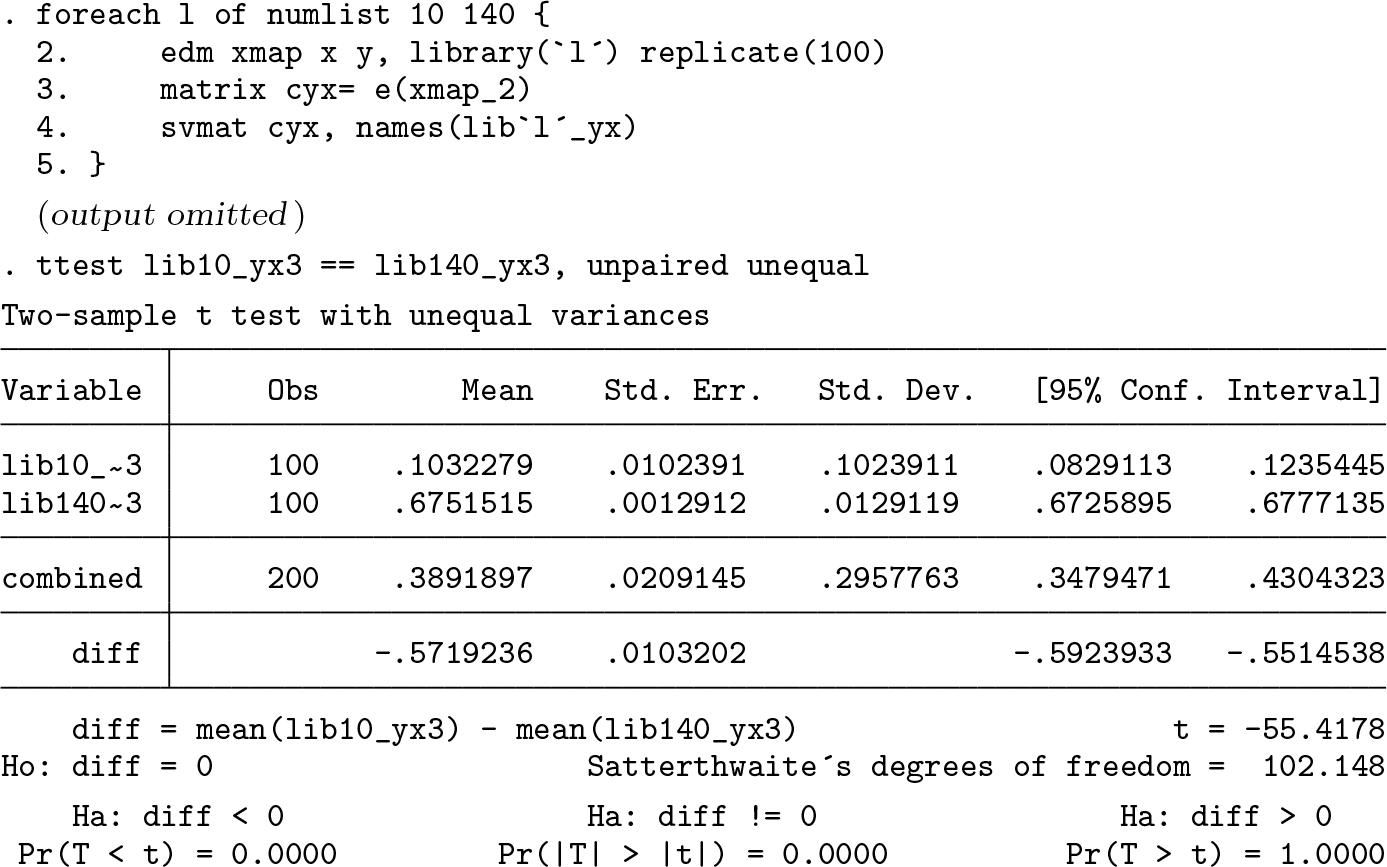
To evaluate convergence for CCM at library sizes smaller than the maximum and for any result from the explore subcommand, a second approach is possible using the replicate() option because the edm program randomly forms the library that defines a reconstructed manifold. Because ρ is expected to increase as L increases during cross-mapping when causality is present, here we give an example testing whether the mean prediction accuracy with a library size of 140 gives statistically significantly better predictions compared with a library size of 10 (that is, a test of convergence).

We randomly sample the dataset 100 times using the replicate() option and test whether the two ρ values stored in rho140_3 and rho10_3 are equal. As shown below, a t test rejects the hypothesis that the mean value of the prediction strength when L = 10 is the same as when L = 140, and in fact the mean ρ of 0.103 increases to 0.675 when increasing L to 140. This indicates that increasing the library size of the reconstructed manifold improves prediction, which can be understood as rejecting a null hypothesis of equivalent predictive ability at small and large library sizes, with an alternative hypothesis of improved prediction at a larger library size (which is consistent with what one may expect for a causal relationship X → Y).

Also relying on the replicate() and i() options, another more common and generally recommended way to test for convergence is to form intervals around ρ or MAE at the minimum L, and see if ρ or MAE at the maximum L is excluded to test for improved prediction (a test for Δρ and ΔMAE; see Ye et al. [2015b] and Ye et al. [2015c]). In such a case, because the test is directional, the estimated ρ and MAE at the maximum library size can be evaluated against whether they fall above the 95% of the distribution at the smallest (or very small) L, perhaps by using replicate(1000), saving all results by using svmat, and then comparing the distributions. Alternatively, one may use the ci() option to get the CIs for the mean values of the ρ estimates.

In the example below, the ci(90) option is used to produce the CI for the mean value of ρ, assuming a normal distribution, as well as the percentile values of the distribution. The first listed CI values for the mean ρ capture the sampling variations associated with the replication or cross-validation estimation process, thus enabling comparisons and hypothesis testing (such as t testing) across different edm (hyper) parameters, including E or L, using the same dataset (that is, making inferences only about the sample itself rather than an external population). The example below shows that even the upper bound of the estimate with a library size of 10 is much lower than the estimate derived at the full library size. The upper bound of 0.1160 for the estimated mean CI and 0.2736 for the observed percentile are well below the observed 0.6968 at the maximum library size—an encouraging sign of convergence for the sample and population, respectively. The percentile values offer a set of alternative metrics, describing the dispersion of the entire distribution of the estimates, which better reflect the expected variation associated with the population.

Similar tests are possible using replicate(1000) with simplex projection at different values of E, and for S-maps to test nonlinearity when θ = 0 versus θ at maximum ρ (or minimum MAE) if these exist when θ > 0 (again, a test of Δρ and ΔMAE; see Hsieh and Ohman [2006], Glaser, Ye, and Sugihara [2013], and Ye et al. [2015a]). For these latter tests, using a common seed() setting will allow pairing the sets of 1,000 replications for θ = 0 versus θ at maximum ρ (or minimum MAE).

Finally, rather than forming intervals around specific ρ or MAE, a third approach forms a null distribution for ρ or MAE by using permutation-based randomization. Typically called a surrogate-data method, this procedure shuffles the data across a time variable (that is, randomizes the time variable) and reestimates the model each time (for example, see Deyle et al. [2016a], Hsieh, Anderson, and Sugihara [2008], and Tsonis et al. [2015]). This is a useful approach because it keeps the observed data intact but ruins its temporal aspects that are essential for modeling system evolution in EDM. With this method, a null distribution can be generated for ρ and MAE in simplex projection, S-mapping, or CCM by simply generating a random sequence of numbers, sorting the data by them, and then generating a new n variable that is tsset as a time indicator (in the panel-data case, using the bysort command with a panel-identifier variable and then xtset).

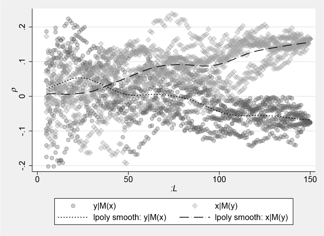
As an example, we can compare figure 6 with the ρ –L convergence in figure 7, which is derived from a permutation test using the original xmap procedure with E = 2 but with randomized timestamps. The figure shows a noisier result with much lower values for ρ, and convergence does not follow a consistent trajectory along the increase of L until very late (close to maximum L). Additionally, the ρ at the full library size still fall within range of the ρ when L is smaller than 50, showing no clear sign of improvement for both directions. (ρ will eventually diverge numerically as estimations become deterministic when the full library is used; thus, the relative differences between the prediction performances in both directions near the full library size alone cannot be used to assess convergence.)

Figure 7.

ρ -L convergence diagnosis in a permutation test

Using this same basic logic, if seasonality or other periodic effects are a concern, permutation can be done in ways that reflect such periodic coupling to test whether these are biasing results (see Deyle et al. [2016a] and Deyle et al. [2016b]).

Beyond these three methods, it is also possible to implement a more traditional nonparametric bootstrap with replacement (see Clark et al. [2015] and Ye et al. [2015c]). Yet, care must be taken in the resampling process because the data must be in a valid time-series or panel format to form the proper E-length vectors without creating missingness. The edm package for Stata does not have this approach built in and it is not planned.

5.6 Evaluating time-delayed causal effects

Another interest when investigating causality is to test for time-delayed causal effects over a specific time frame. Ye et al. (2015b) proposed an extension of CCM to determine whether a driving variable acts with some time delay on a response variable by explicitly considering different lags for cross-mapping. In this approach, one implication is that direct effects among variables should have the highest cross-map skill (that is, largest ρ and smallest MAE) and the most immediate effects (no or few lags). On the other hand, indirect effects should be weaker and have longer time delays. Furthermore, and rather curiously, in cases where bidirectional causality appears to exist because of what is actually strong unidirectional forcing, an impossible positive lag showing a maximum effect can indicate false convergence (see Ye et al. [2015b])—in this case, the test for time-delayed effects is thus an assumption test.

The edm command supports such reverse- and forward-lagged analyses with minimal input changes by relying on time-series operators (prefixes l.and f.). To illustrate this, we introduce a new variable z,

z_{t} = z_{t}_{- 1} {3.77 (1 - z_{t}_{- 1}) - 0.4 y_{t}_{- 1}}

which is a function of its own past values and the lagged values from y, thus forming an indirect x → y → z effect. We use edm to test direct causation between x, y, and z by estimating their time-delayed CCM performance.

As shown in the cross-mapping results⁷ in figure 8, x → y and y → z seem to exhibit higher ρ values and fewer delays. The link between x and z has much weaker cross-map skill and longer delays in observing the peak ρ, suggesting an indirect time-delayed causal effect that by design exists in our model: x → y → z.

Figure 8.

Time-delayed causal detection

5.7 Visualizing the strength of causation

To demonstrate the usefulness of EDM in estimating the impact of causal variables, in this section we use a real-world dataset (available with the article files) that reflects daily temperature and crime levels in Chicago. Compared with the previous logistic map example, where the marginal effects of the two variables are highly unstable over time by construction, this example showcases how edm can be applied in a real-world dataset.

We first use the steps we recommended above: explore the data series 1) using simplex projection to find optimal E and 2) using S-maps to examine for nonlinearity. Then 3) use the xmap subcommand to conduct CCM and examine for convergence to test causality among the series. Following this, we can 4) run the xmap subcommand with the algorithm(smap) option to derive regression coefficients that can be used to estimate bivariate overall causal effects.

In the exploration phase, edm suggests that temperature and crime have an optimal E of 7, which was determined by using the command edm explore temp, e(2/20) crossfold(5) to find the largest ρ. The crossfold() option offers more refined control over the training/testing data split ratio and in this case reports the results from a five-fold cross-validation.⁸ Similar to the replicate() implementation, training/test data split applies at the manifold instead of at the observation level to avoid introducing additional gaps in the time series, allowing more refined control over the split ratio.

Figure 9 shows the ρ –L convergence plot derived from the edm xmap return matrices.⁹ As shown, CCM suggests the likely causal direction is that an increase in temperature leads to a change in crime rate rather than the reverse (and impossible) case of crime affecting temperature. Consistent with existing findings using more typical methods, this analysis suggests that temperature CCM-causes crime.

Figure 9.

ρ –L convergence plot for Chicago crime dataset (10 replications)

To estimate the size of causal effects in addition to predictive ability in CCM, we proceed with cross-mapping using the S-map algorithm and the savesmap() option, which saves estimated coefficients that indicate the marginal effects of the variables. The command used in the analysis is as follows, where the k(-1) option is used to recruit all available neighbors in the reconstructed manifold for prediction with a default weighting theta(1). Specifying a positive number in the k() option would restrict the number of neighbors, reducing computation times. However, a low value results in less stable results given the smaller sample size in the local regressions.

In addition to the standard reporting, this command generates new variables named with the prefix beta that provide marginal regression coefficients across all points in the prediction library for the variables listed. Recall from above that to obtain the marginal regression coefficients in the typical predictor → outcome direction for regression will require reversing the order of the variables, because CCM causality is evaluated in the opposite direction. Thus, in this example, we only use variables starting with beta1 given that our interest is in the marginal effect of temperature in a manifold when predicting crime, and the command edm xmap temp crime will generate the prediction crime| M _temp for the beta1 coefficients. This differs from the CCM causal exploration earlier, where we used the manifold constructed by the crime variable to infer the causal effect of temperature on crime, or temp| M _crime.¹⁰ Because no replicate() option is specified, all beta variables share the same suffix, rep1(first replication), and replication is not relevant because the library size is at a maximum.

As explained earlier, the S-map process uses what can be thought of as a locally weighted distributed lag model with E predictors (and a constant term c), and each of the coefficients can be stored as variables with the savesmap() option. Recall the naming convention detailed in the savesmap() option description in section 3, wherein numbers after b indicate the length of the lag (from 0 to E − 1). Recall also that these coefficients are saved for each predicted value and are appropriately matched in a dataset to the observation t that is being predicted. In other words, each observation in a dataset at t ≥ E will have E + 1 regression weights associated with it, where each reflects the E weights on the k neighbors from the library set and the constant used for prediction. In this example, e(7) produces eight coefficients¹¹ (seven for lags and one constant) for each predicted observation in the dataset at t ≥ 7. Other possible embedding combinations may lead to different estimates for the same variable, although the results are expected to be broadly consistent because they reflect the same underlying dynamic system. Again, we emphasize that results should be understood in this light rather than in terms of a typical regression model.

Figure 10 plots the contemporaneous effect of temperature on crime (beta1_b1_rep1) in the local S-map prediction together with the temperature. The contemporaneous effect, as shown, is distributed between 2 and 5 and suggests an average increase of approximately 3.3 crimes¹² per degree of temperature rise. This is akin to the marginal contemporaneous effect of temperature on crime in a local regression. Each dot in the figure represents one estimate in the local state space of an observation. Given the nonlinearity of the model, the coefficients from different states are not necessarily the same. In this case, we observe a gradually declining effect of temperature on crime as the weather becomes warmer. These coefficients describe expected changes in crime rates at different temperatures rather than expected crime rates themselves (which tend to be higher during warmer days). Similar to a standard regression, the coefficient size should be interpreted in the context of the unit of measurement for the observed variables. If the z.prefix is added to the variable names, the results should be interpreted as changes in the standardized score, similar to a standardized regression coefficient.

Figure 10.

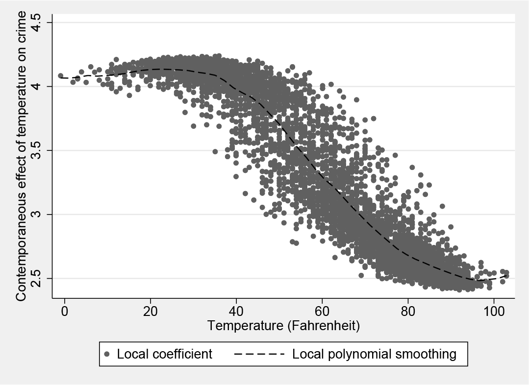
Scatterplot of the S-map coefficient (contemporaneous effect)

Depending on the context of the analysis, it could also be important to emphasize the dynamic nature of the model, because any change at t−τ would affect the observations at time t. To predict the impact of a lagged temperature shock, one may consider running the prediction iteratively over time (a step-ahead prediction) to estimate its long-term impact on crime rate. The prediction via this dynamic process may be different than the reported coefficients because of the nonlinear nature of the system. The more common practice in autoregressive or VAR models of using the sum of the average effects across all E lags may ignore the nonlinear dynamics in the marginal effects over time.

To illustrate the use of the command, we also provide three template do-files as part of the supplementary materials for the article. These cover three common analysis types for time-series data, “multispatial” panel data (a shared dynamic system using the default multispatial approach), and “multiple EDM” panel data (distinct dynamic systems where each panel is analyzed separately; similar to van Berkel et al. [Forthcoming]). These do-files automatically analyze data using the primary EDM tools of simplex projection, S-maps, and CCM but also produce various plots and automate additional postprocessing, including hypothesis tests of various types. These do-files will also be updated over time to include additional features and fix bugs.

6 Concluding remarks

The new edm package for Stata offers nonparametric tools for characterizing and modeling causality in nonlinear dynamic systems. It allows users to explore the bivariate overall causal relationships among variables with minimal assumptions on the data-generation process. The package includes the common tools for causal explorations for a typical end user. For advanced users, the command exports several useful Stata locals and matrices for postprocessing. Combined with the capacity of Stata’s other built-in and community-contributed commands, the new edm command offers a relatively easy interface for relatively complex EDM computations as well as the ability to fine-tune the critical parameters behind EDM analyses. Thus, the procedure implemented in this package can be applied in datasets collected in many different fields, including health science, psychology, economics, sociology, and the natural sciences.

This is an important addition to Stata’s existing capabilities for multiple reasons, including checking the assumptions that underlie many existing time-series and panel-data methods. For example, most of these methods assume stability or stationarity in random residuals, but tests for these conditions are typically based on assumptions of linearity and therefore may not be sensitive to nonlinear dynamics. To evaluate this, residuals from typical approaches can be subjected to the methods we propose here to check for structure from nonlinear dynamic systems (Dixon, Milicich, and Sugihara [2001]; see also Glaser et al. [2011]). Specifically, simplex projection can be used to test for low-dimensional determinism that may masquerade as random noise, and S-maps can be used to test for nonlinearity. Furthermore, residuals and observed predictors can be used in CCM to test for causal effects missed in other approaches, whereas all residuals from VAR models can be used in CCM for the same purpose. This allows for more robust tests of assumptions regarding residual dynamic structures.

Like many community-contributed programs, edm is a work in progress with new features to appear in future versions (along with bug fixes). As a nonparametric method, the command may require considerable computing time when running on large datasets, even with the core algorithm coded in the Mata language and run on multiple CPU cores in Stata/MP. Future updates will explore further optimization possibilities and better leverage the multiple cores in modern architectures, including on graphics processing units. Additionally, the integration of imputation techniques will also be considered and implemented in future versions. The help file of the edm command will describe these improvements as we proceed, elaborating on this important initial work for nonlinear dynamic systems modeling in Stata. Our goal is to provide the kinds of tools required to address the complex systems that social and health scientists increasingly recognize as being ubiquitous in their fields of study (for example, Atkinson et al. [2018] and Rutter et al. [2017]), while improving computation times to better tackle the “big data” problems that are increasingly found across the social, health, and natural sciences.

Supplemental Material

Supplemental Material, sj-zip-1-stj-10.1177_1536867X211000030 - Beyond linearity, stability, and equilibrium: The edm package for empirical dynamic modeling and convergent cross-mapping in Stata

Supplemental Material, sj-zip-1-stj-10.1177_1536867X211000030 for Beyond linearity, stability, and equilibrium: The edm package for empirical dynamic modeling and convergent cross-mapping in Stata by Jinjing Li, Michael J. Zyphur, George Sugihara and Patrick J. Laub in The Stata Journal

Footnotes

7 Acknowledgments

This research was supported partially by the Australian Government through the Australian Research Council’s Discovery Projects and Future Fellowship funding scheme (projects DP200100219 and FT140100629). The views expressed herein are those of the authors and are not necessarily those of the Australian Government or Australian Research Council.

8 Programs and supplemental materials

To install a snapshot of the corresponding software files as they existed at the time of publication of this article, type

Notes

References

Atkinson

J.-A.

Page

Prodan

McDonnell

Osgood

2018. Systems modelling tools to support policy and planning. Lancet 391: 1158–1159. https://doi.org/10.1016/s0140-6736(18)30302-7.

Chang

C.-W.

Ushio

Hsieh

2017. Empirical dynamic modeling for beginners. Ecological Research 32: 785–796. https://doi.org/10.1007/s11284-017-1469-9.

Clark

A. T.

2014. multispatialCCM: Multispatial convergent cross mapping. R package version 1.0. https://cran.r-project.org/web/packages/multispatialCCM/.

Clark

A. T.

Isbell

Deyle

E. R.

Cowles

Tilman

G. D.

Sugihara

2015. Spatial convergent cross mapping to detect causal relationships from short time series. Ecology 96: 1174–1181. https://doi.org/10.1890/14-1479.1.

Deyle

E. R.

Fogarty

Hsieh

C.-h.

Kaufman

MacCall

A. D.

Munch

S. B.

Perretti

C. T.

Sugihara

2013. Predicting climate effects on Pacific sardine. Proceedings of the National Academy of Sciences 110: 6430–6435. https://doi.org/10.1073/pnas.1215506110.

Deyle

E. R.

Maher

M. C.

Hernandez

R. D.

Basu

Sugihara

2016a. Global environmental drivers of influenza. Proceedings of the National Academy of Sciences 113: 13081–13086. https://doi.org/10.1073/pnas.1607747113.

Deyle

E. R.

May

R. M.

Munch

S. B.

Sugihara

2016b. Tracking and forecasting ecosystem interactions in real time. Proceedings of the Royal Society B: Biological Sciences 283: 20152258. https://doi.org/10.1098/rspb.2015.2258.

Deyle

E. R.

Sugihara

2011. Generalized theorems for nonlinear state space reconstruction. PLOS ONE 6: e18295. https://doi.org/10.1371/journal.pone.0018295.

Dixon

P. A.

Milicich

M. J.

Sugihara

1999. Episodic fluctuations in larval supply. Science 283: 1528–1530. https://doi.org/10.1126/science.283.5407.1528.

10.

Dixon

P. A.

Milicich

M. J.

Sugihara

2001. Noise and nonlinearity in an ecological system. In Nonlinear Dynamics and Statistics, ed. A. I. Mees, 339–364. Boston: Birkh¨auser. https://doi.org/10.1007/9781-4612-0177-9_14.

11.

Glaser

S. M.

Maunder

MacCall

Fogarty

Sugihara

2011. Detecting and forecasting complex nonlinear dynamics in spatially structured catch-per-unit-effort time series for North Pacific albacore (Thunnus alalunga). Canadian Journal of Fisheries and Aquatic Sciences 68: 400–412. https://doi.org/10.1139/f10-160.

12.

Glaser

S. M.

Sugihara

2013. A nonlinear, low data requirement model for producing spatially explicit fishery forecasts. Fisheries Oceanography 23: 45–53. https://doi.org/10.1111/fog.12042.

13.

Hsieh

Anderson

Sugihara

2008. Extending nonlinear analysis to short ecological time series. American Naturalist 171: 71–80. https://doi.org/10.1086/524202.

14.

Hsieh

Ohman

M. D.

2006. Biological responses to environmental forcing: The linear tracking window hypothesis. Ecology 87: 1932–1938. https://doi.org/10.1890/0012-9658(2006)87[1932:brteft]2.0.co;2.

15.

Jackson

E. A.

Hübler

1990. Periodic entrainment of chaotic logistic map dynamics. Physica D: Nonlinear Phenomena 44: 407–420. https://doi.org/10.1016/0167-2789(90)90155-i.

16.

Leng

Kurths

Lai

Y.-C.

Lin

Aihara

Chen

2020. Partial cross mapping eliminates indirect causal influences. Nature Communications 11: 2632. https://doi.org/10.1038/s41467-020-16238-0.

17.

May

R. M.

1976. Simple mathematical models with very complicated dynamics. Nature 261: 459–467. https://doi.org/10.1038/261459a0.

18.

Mønster

Fusaroli

Tylén

Roepstorff

Sherson

J. F.

2017. Causal inference from noisy time-series data—Testing the convergent cross-mapping algorithm in the presence of noise and external influence. Future Generation Computer Systems 73: 52–62. https://doi.org/10.1016/j.future.2016.12.009.

19.

Perretti

C. T.

Munch

S. B.

Sugihara

2013. Model-free forecasting outperforms the correct mechanistic model for simulated and experimental data. Proceedings of the National Academy of Sciences 110: 5253–5257. https://doi.org/10.1073/pnas.1216076110.

20.

Rodriguez

J. D.

Perez

Lozano

J. A.

2010. Sensitivity analysis of k-fold cross validation in prediction error estimation. IEEE Transactions on Pattern Analysis and Machine Intelligence 32: 569–575. https://doi.org/10.1109/tpami.2009.187.

21.

Rutter

Savona

Glonti

Bibby

Cummins

Finegood

D. T.

Greaves

Harper

Hawe

Moore

Petticrew

Rehfuess

Shiell

Thomas

White

2017. The need for a complex systems model of evidence for public health. Lancet 390: 2602–2604. https://doi.org/10.1016/s0140-6736(17)31267-9.

22.

Sauer

Yorke

J. A.

Casdagli

1991. Embedology. Journal of Statistical Physics 65: 579–616. https://doi.org/10.1007/bf01053745.

23.

Schiff

S. J.

Chang

Burke

R. E.

Sauer

1996. Detecting dynamical interdependence and generalized synchrony through mutual prediction in a neural ensemble. Physical Review E 54: 6708–6724. https://doi.org/10.1103/physreve.54.6708.

24.

Stark

1999. Delay embeddings for forced systems. I. deterministic forcing. Journal of Nonlinear Science 9: 255–332. https://doi.org/10.1007/s003329900072.

25.

Stark

Broomhead

D. S.

Davies

M. E.

Huke

2003. Delay embeddings for forced systems. II. Stochastic forcing. Journal of Nonlinear Science 13: 519–577. https://doi.org/10.1007/s00332-003-0534-4.

26.

Sugihara

1994. Nonlinear forecasting for the classification of natural time series. Philosophical Transactions of the Royal Society of London, Series A 348: 477–495. https://doi.org/10.1098/rsta.1994.0106.

27.

Sugihara

May

Hsieh

C.-h.

Deyle

Fogarty

Munch

2012. Detecting causality in complex ecosystems. Science 338: 496–500. https://doi.org/10.1126/science.1227079.

28.

Sugihara

May

R. M.

1990. Nonlinear forecasting as a way of distinguishing chaos from measurement error in time series. Nature 344: 734–741. https://doi.org/10.1038/344734a0.

29.

Takens

1981. Detecting strange attractors in turbulence. In Dynamical Systems and Turbulence, ed. D. Rand and L.-S. Young, 366–381. Berlin: Springer. https://doi.org/10.1007/BFb0091924.

30.

Tsonis

A. A.

Deyle

E. R.

May

R. M.

Sugihara

Swanson

Verbeten

J. D.

Wang

2015. Dynamical evidence for causality between galactic cosmic rays and interannual variation in global temperature. Proceedings of the National Academy of Sciences 112: 3253–3256. https://doi.org/10.1073/pnas.1420291112.

31.

van Berkel

Dennis

Zyphur

Heathcote

Kostakos

. Forth-coming. Modeling interaction as a complex system. Human–Computer Interaction. https://doi.org/10.1080/07370024.2020.1715221.

32.

van Dijk

Sharma

Nainys

Yim

Kathail

Carr

A. J.

Burdziak

Moon

K. R.

Chaffer

C. L.

Pattabiraman

Bierie

Mazutis

Wolf

Krishnaswamy

Pe’er

2018. Recovering gene interactions from single-cell data using data diffusion. Cell 174: 716–729. https://doi.org/10.1016/j.cell.2018.05.061.

33.

van Nes

E. H.

Scheffer

Brovkin

Lenton

T. M.

Deyle

Sugihara

2015. Causal feedbacks in climate change. Nature Climate Change 5: 445–448. https://doi.org/10.1038/nclimate2568.

34.

Beamish

R. J.

Glaser

S. M.

Grant

S. C. H.

Hsieh

Richards

L. J.

Schnute

J. T.

Sugihara

2015a. Equation-free mechanistic ecosystem forecasting using empirical dynamic modeling. Proceedings of the National Academy of Sciences 112: E1569–E1576. https://doi.org/10.1073/pnas.1417063112.

35.

Clark

Deyle

Sugihara

2016. rEDM: An R package for empirical dynamic modeling and convergent cross mapping. https://ha0ye.github.io/rEDM/articles/rEDM.html.

36.

Deyle

E. R.

Gilarranz

L. J.

Sugihara

2015b. Distinguishing time-delayed causal interactions using convergent cross mapping. Scientific Reports 5: 14750. https://doi.org/10.1038/srep14750.

37.

Sugihara

2016. Information leverage in interconnected ecosystems: Overcoming the curse of dimensionality. Science 353: 922–925. https://doi.org/10.1126/science.aag0863.

38.

Sugihara

Deyle

E. R.

May

R. M.

Swanson

Tsonis

A. A.

2015c. Reply to Luo et al.: Robustness of causal effects of galactic cosmic rays on interannual variation in global temperature. Proceedings of the National Academy of Sciences 112: E4640–E4641. https://doi.org/10.1073/pnas.1511080112.

Supplementary Material

Please find the following supplemental material available below.

For Open Access articles published under a Creative Commons License, all supplemental material carries the same license as the article it is associated with.

For non-Open Access articles published, all supplemental material carries a non-exclusive license, and permission requests for re-use of supplemental material or any part of supplemental material shall be sent directly to the copyright owner as specified in the copyright notice associated with the article.

0.02 MB

0.00 MB

Beyond linearity,stability,and equilibrium: The edm package for empirical dynamic modeling and convergent cross-mapping in Stata

Abstract

Keywords

1 Introduction

2 Method

2.1 Simplex projection

2.2 S-maps

2.3 CCM

2.4 Missing data and sample-size considerations

3 Syntax

3.1 Options

4 Output and stored results

5 Examples

5.1 Creating a dynamic system

5.2 Exploring the system’s dimensionality

5.3 Nonlinearity detection using S-map

5.4 Causality detection using CCM

5.5 Hypothesis testing with CIs and null distributions

5.6 Evaluating time-delayed causal effects

5.7 Visualizing the strength of causation

6 Concluding remarks

Supplemental Material

Supplemental Material, sj-zip-1-stj-10.1177_1536867X211000030 - Beyond linearity, stability, and equilibrium: The edm package for empirical dynamic modeling and convergent cross-mapping in Stata

Footnotes

7 Acknowledgments

8 Programs and supplemental materials

Notes

References

Supplementary Material