msreg: A command for consistent estimation of linear regression models using matched data

Abstract

Economists often use matched samples, especially when dealing with earning data where some observations are missing in one sample and need to be imputed from another sample. Hirukawa and Prokhorov (2018, Journal of Econometrics 203: 344–358) show that the ordinary least-squares estimator using matched samples is inconsistent and propose two consistent estimators. We describe a new command, msreg, that implements these two consistent estimators based on two samples. The estimators attain the parametric convergence rate if the number of continuous matching variables is no greater than four.

1 Introduction

Matching-based imputation is common in economic datasets. For example, the U.S. Census uses a practice known as “hot-deck imputation”, which is implemented when census reports for nonresponders the values of important variables such as earnings and income are borrowed from responders with a few similar characteristics. In some surveys, the share of such imputed responses reaches 30%.

Hirukawa and Prokhorov (2018) were concerned with this widely used but often ignored practice. The concern was that users of such data in applied econometrics are often unaware that these are imputed, rather than actual, observations and that the resulting matching discrepancy leads to nonnegligible biases in the ordinary least-squares (OLS) estimator. They list many other settings, usually involving more than one dataset, where matching is unavoidable and needs to be accounted for.

The goal of this article is to facilitate the use of the consistent estimation approaches proposed by Hirukawa and Prokhorov (2018) in their numerous applications. Hirukawa and Prokhorov (2018) derive the imputation bias analytically and propose two bias-corrected estimators. In this article, we introduce a new command, msreg, that implements both estimators in Stata.

Section 2 documents theoretical backgrounds for the msreg command. Section 3 discusses the msreg syntax and provides a numerical example. Section 4 contains a simulation study. Section 5 provides an empirical application by estimating the return to schooling as in Hirukawa and Prokhorov (2018).

2 Setup and estimators

2.1 Setup and assumptions

Suppose that we are interested in fitting a linear regression model,

$y={\beta }_0+x_1^{\prime }{\beta }_1+x_2^{\prime }{\beta }_2+z^{\prime }\gamma +u=w^{\prime }\theta +u\hspace{1em}E(u\mid w)=0$

where $x_1\in R^{d_1},x_2\in R^{d_2},z\in R^{d_z}$ , $w=\left(1,x_1^{\prime },x_2^{\prime },z^{\prime }\right)$ , and $\theta ={\left({\beta }_0,{\beta }_1^{\prime },{\beta }_2^{\prime },{\gamma }^{\prime }\right)}^{\prime }$ .

If we can observe all the variables in one sample, OLS is a consistent estimator for θ . However, in reality, we often encounter a situation where the variables are taken from two different samples. To be precise, we need more notation to distinguish between the two samples. The first sample is denoted by $S_1={\left\{\left(y_i,x_{1i},z_i\right)\right\}}_{i=1}^n$ . The second sample is denoted by $S_2={\left\{\left(x_{2j},z_j\right)\right\}}_{j=1}^m$ . For inference, we also denote d ₃ as the number of continuous common variables in z hereafter, which is not always equal to d_z .

Estimation theories in Hirukawa and Prokhorov (2018) are built on a set of assumptions that are required for identification, consistency, and asymptotic normality of their estimators. Some of them are quite common. For example, assumption 2 imposes compactness of the support of continuous common variables. In our empirical analysis in section 5, educ, feduc, and meduc are such variables, and it is natural to think of their support as compact. On the other hand, there are more subtle assumptions in Hirukawa and Prokhorov (2018) that may or may not hold in a given application. Examples include a common joint distribution for S ₁ and S ₂ (assumption 1), $E\left({\eta }_1{\eta }_2^{\prime }\right)=0$ and strict nonlinearity in g ₂ (·) [assumption 3(ii)], where η _ℓ := x _ℓ − g_ℓ (z) and g_ℓ (z) := E (x _ℓ| z) for ℓ = 1, 2. It is difficult to test the validity of these assumptions because x ₁ and x ₂ belong to two distinct samples.

2.2 Nearest-neighbor matching

The matched sample can be constructed via the nearest-neighbor matching (NNM) using a vector of common variables z across two samples. Note that z must contain at least one continuous variable for valid inference; inclusion of discrete common variables with a finite number of support points (for example, binary variables) in z does not affect the asymptotic results that will be stated shortly.

To specify the NNM, we need to first define a matrix norm to measure the distance between two vectors. For a vector x and some symmetric and positive definite matrix A, the vector norm is defined as || x || _A = (x ^′ Ax)^{1 / 2}. Following Abadie and Imbens (2011), we use the Mahalanobis metric $A_M={\left\{(1/N){\displaystyle {\sum }_{i=1}^N\left(z_i-\overline{z}\right){\left(z_i-\overline{z}\right)}^{\prime }}\right\}}^{-1}$ and the normalized Euclidean metric $A_{NE}=diag{\left(A_M^{-1}\right)}^{-1}$ , where N = n + m and $\overline{z}=(1/N){\displaystyle {\sum }_{i=1}^N{z}_i}$ .

Let j_k (i) be the index of the kth match in S ₂ to the unit i in S ₁; that is, for each i ∊ {1,…, n}, j_k (i) satisfies

${\displaystyle \sum _{j=1}^m\mathbb{1}\left\{\text{||}{z}_j-z_i{\text{||}}_A\le \text{||}{z}_{j_k(i)}-z_i{\text{||}}_A\right\}=k}$

In other words, $z_{j_k(i)}$ is the kth nearest neighbor in S ₂ to the unit i in S ₁.

For each unit i, let J _K (i) = {j_i (1),…, j_i (K)} denote the K matches from S ₂. The NNM-based matched sample is

$S={\left\{\left(y_i,x_{1i},x_{2j_1(i)},\dots ,x_{2j_K(i)},z_i\right)\right\}}_{i=1}^n$

We also write $\overline{x_{2j(i)}}=(1/K){\displaystyle {\sum }_{j\in J_K(i)}{x}_{2j}}$ .

For estimation, we use a transformation of the matched sample S.

$S^{\ast }={\left\{\left(y_i,x_{1i},\overline{x_{2j(i)}},z_i\right)\right\}}_{i=1}^n$

In contrast with the original matched sample S, we replace the individual matched variable $x_{2j_1(i)},\dots ,x_{2j_K(i)}$ by its mean $\overline{x_{2j(i)}}$ .

Throughout, it is assumed that we estimate θ by regressing y_i on $w_{i,j(i)}={\left(1,x_{1i}^{\prime },{\overline{x_{2j(i)}}}^{\prime },z_i\right)}^{\prime }$ .

2.3 Inconsistency of matched-sample OLS

We start by using an OLS estimator on the matched sample S ^∗. The OLS estimator is

${\widehat{\theta }}_{\text{MSOLS}}={\widehat{Q_W}}^{-1}\widehat{R_W}$

where $\widehat{Q_W}=(1/n){\displaystyle {\sum }_{i=1}^n{w}_{i,j(i)}{w}_{i,j(i)}^{\prime }}$ and $\widehat{R_W}=(1/n){\displaystyle {\sum }_{i=1}^n{w}_{i,j(i)}{y}_i}$ . It is referred to as the matched-sample OLS (MSOLS) estimator.

Theorem 1 (Hirukawa and Prokhorov [2018], theorem 1). Under some regularity conditions,

${\widehat{\theta }}_{\text{MSOLS}}=Q_W^{-1}{P}_W\theta +O_p\left(m^{-1/d_3}\right)+O_p\left(n^{-1/2}\right)$

where $Q_W=E\left(w_{i,j(i)}{w}_{i,j(i)}^{\prime }\right)$ , P _W = Q _W − (1/K)Σ, Σ is a (d + 1) × (d + 1) block-diagonal matrix of the form $\Sigma =diag\left\{0_{\left(d_1+1\right)\times \left(d_1+1\right)},{\Sigma }_2,0_{d_z\times d_z}\right\}$ , and ${\Sigma }_2=E\left({\eta }_2{\eta }_2^{\prime }\right)$ .

Theorem 1 implies that MSOLS is inconsistent in general. The inconsistency is attributed to correlation between the imputed regressor $\overline{x_{2j(i)}}$ and $(1/K){\displaystyle {\sum }_{j\in J_{K(i)}}{\eta }_{2j}}$ in the composite error term ⲉ_{i,j ( i )}. All asymptotic analyses in Hirukawa and Prokhorov (2018) are based on letting n and m diverge while keeping K fixed. It is in principle possible to restore consistency by letting K diverge at a rate slower than n and m. However, a fixed K is what researchers are likely to do in practice; Abadie and Imbens (2006) also adopt this setup. Moreover, the $O_p\left(m^{-1/d_3}\right)$ term corresponds to the second-order bias term λ_{i,j ( i )} because of the matching discrepancy of Abadie and Imbens (2006). Observe that this term affects the convergence rate of ${\widehat{\theta }}_{\text{MSOLS}}$ to its probability limit; see remark 3 of Hirukawa and Prokhorov (2018) for more details.

2.4 One-step bias-corrected estimator

The source of the inconsistency of the MSOLS estimator is that $\widehat{Q_W}\stackrel{p}{\to }{Q}_W$ , whereas $\widehat{R_W}\stackrel{p}{\to }{P}_W\theta =\left\{Q_W-(1/K)\Sigma \right\}\theta$ . To eliminate the nonvanishing bias, we replace the denominator $\widehat{Q_W}$ by a consistent estimator of P _W and leave the numerator $\widehat{R_W}$ unchanged. Because this bias correction has an indirect inference interpretation, Hirukawa and Prokhorov (2018) call this estimator the matched-sample indirect inference (MSII) estimator. Let $\widehat{P_W}$ be some consistent estimator of P _W . Then, the MSII estimator is defined as

${\widehat{\theta }}_{\text{MSII}}={\widehat{P_W}}^{-1}\widehat{R_W}$

To consistently estimate P _W , we need consistent estimators for Q _W and Σ. Apparently, $\widehat{Q_W}$ is a natural estimator for Q _W . Furthermore, it turns out that we can consistently estimate Σ without nonparametric estimation of E(x ₂ | z). To do so, we first reorder S ₂ with respect to z in ascending order.

Define z _{( 1 )} as the observation that has the smallest first element; that is, (1) = arg min_{1 ≤ j ≤ m} z _{j 1}.

For j = 2,…, m, choose (j) = arg min _{j ≠ ( 1 ) ,…, ( j − 1 )} || z _j − z _{( j − 1 )} ||, where the norm of a matrix || A || is defined as || A || = {tr(A ^′ A)}^{1 / 2}.

Given the reordered sample $S_2={\left\{\left(x_{2(j)},z_{(j)}\right)\right\}}_{j=1}^m$ , Σ ₂ can be consistently estimated by

$\widehat{{\text{Σ}}_2}=\frac{1}{2(m-1)}{\displaystyle \sum _{j=2}^m\text{Δ}{x}_{2(j)}\text{Δ}{x}_{2(j)}^{\prime }}$

where Δx _{2 ( j )} = x _{2 ( j )} − x _{2 ( j − 1 )}. This is known as the difference-based variance estimator; see von Neumann (1941), Yatchew (1997), and Horowitz and Spokoiny (2001) for references.

The estimator of P _W is given by

$\widehat{P_W}=\widehat{Q_W}-\frac{1}{K}\widehat{\Sigma }=\widehat{Q_W}-\frac{1}{K}\text{diag}\left\{0_{\left(d_1+1\right)\times \left(d_1+1\right)},\widehat{{\Sigma }_2},0_{d_z\times d_z}\right\}$

Theorem 2 below documents asymptotic normality of ${\widehat{\theta }}_{\text{MSII}}$ . The theorem applies only when the number of continuously distributed matching variables is so small that the second-order, matching discrepancy bias can be safely ignored. Observe that both the convergence rate of ${\widehat{\theta }}_{\text{MSII}}$ and its asymptotic variance depend on the divergence pattern of (n, m).

Theorem 2 (Hirukawa and Prokhorov [2018], Corollary 1). Under some regularity conditions, as n, m → ∞,

$\{\begin{array}{ll}\sqrt{n}\left({\widehat{\theta }}_{\text{MSII}}-\theta \right)\stackrel{d}{\to }N\left(0,V_I\right)=N\left(0,P_W^{-1}\Omega P_W^{-1}\right)\hfill & \begin{array}{l} if n/m\to \kappa \in (0,\infty )\hfill \\ \hspace{0.17em}\hspace{0.17em}\hspace{0.17em}\hspace{0.17em}\text{and }{d}_3=1\hfill \end{array}\hfill \\ \sqrt{n}\left({\widehat{\theta }}_{\text{MSII}}-\theta \right)\stackrel{d}{\to }N\left(0,V_{II}\right)=N\left(0,P_W^{-1}{\Omega }_{11A}{P}_W^{-1}\right)\hfill & \begin{array}{l} if n/m\to 0\hfill \\ \hspace{0.17em}\hspace{0.17em}\hspace{0.17em}\hspace{0.17em}\text{and }{d}_3=\mathrm{1,2}\hfill \end{array}\hfill \\ \sqrt{m}\left({\widehat{\theta }}_{\text{MSII}}-\theta \right)\stackrel{d}{\to }N\left(0,V_{III}\right)=N\left(0,P_W^{-1}{\Omega }_{22}{P}_W^{-1}\right)\hfill & \begin{array}{l} if n/m\to \infty \hfill \\ \hspace{0.17em}\hspace{0.17em}\hspace{0.17em}\hspace{0.17em}\text{and }{d}_3=1\hfill \end{array}\hfill \end{array}$

where the definitions of Ω, Ω _{11 A}, and Ω ₂₂ can be found in the appendix, along with their consistent estimates.

As demonstrated in this theorem and theorem 3 below, the bias-corrected estimators of Hirukawa and Prokhorov (2018) attain the parametric convergence rate only when the number of continuous common variables is four or less. It may be tempting to include as many continuous common variables as possible in the NNM. However, this results in slowing down the convergence rate, and we do not recommend it.

2.5 Two-step bias-corrected estimator

The one-step bias-corrected estimator can attain the parametric rate of convergence with at most two matching variables. To overcome this curse of dimensionality, we should eliminate the second-order bias λ_{i,j ( i )}. The entire procedure is reminiscent of the fully modified least-squares estimation for cointegrating regressions by Phillips and Hansen (1990). In this sense, Hirukawa and Prokhorov (2018) call the estimator the fully modified MSII (MSII-FM) estimator.

Estimating λ_{i,j ( i )} requires consistent estimates of θ and g ₂(·). For θ , we can use the MSII estimate ${\widehat{\theta }}_{\text{MSII}}$ . For g ₂(·), we use a nonparametric power-series estimation as in Abadie and Imbens (2011). Let $v=\left(v_1,\dots ,v_{d_z}\right)$ be a multi-index of dimension d_z , which is a d_z -dimensional vector of nonnegative integers with $|v|\hspace{0.17em}=\hspace{0.17em}{\displaystyle {\sum }_{l=1}^{d_z}{v}_l}$ . Also, denote $z^v={\text{Π}}_{l=1}^{d_z}{z}_l^{v_l}$ . Consider a series ${\left\{v_Q\right\}}_{Q=1}^{\infty }$ containing distinct vectors such that |v(Q)| is nondecreasing. Let p_Q (z) = z ^{v ( Q )} and p^Q (z) = {p ₁(z),…, p_Q (z)} ^′ . Then, a nonparametric series estimator of the regression function g _{2 r} (z), r = 1,…, d ₂ is

$\widehat{g_{2r}}=p^{Q(m)}(z{)}^{\prime }{\left\{{\displaystyle \sum _{j=1}^m{p}^{Q(m)}\left(z_j\right)p^{Q(m)}{\left(z_j\right)}^{\prime }}\right\}}^{-}{\displaystyle \sum _{j=1}^m{p}^{Q(m)}\left(z_j\right)x_{2r,j}}$

where x _{2 r,j} denotes the rth element of x _{2 j} in S ₂, (·)⁻ denotes the generalized inverse, and Q = Q(m) implies the dependence of Q on the sample size of S ₂.

The entire estimation procedure can be summarized in the following three steps:

1. Run MSII using the matched sample S ^∗ to obtain

${\widehat{\theta }}_{\text{MSII}}={\left({\widehat{{\beta }_{II,0}}}^{\prime },{\widehat{{\beta }_{II,1}}}^{\prime },{\widehat{{\beta }_{II,2}}}^{\prime },{\widehat{{\gamma }_{II}}}^{\prime }\right)}^{\prime }$

2. Construct adjusted dependent variables ${\left\{y_i^{+}\right\}}_{i=1}^n={\left\{y_i-{\widehat{\lambda }}_{i,j(i)}\right\}}_{i=1}^n$ , where

${\widehat{\lambda }}_{i,j(i)}={\left(\widehat{g_2}\left(z_i\right)-\frac{1}{K}{\displaystyle \sum _{j\in J_K(i)}{\widehat{g}}_2\left(z_j\right)}\right)}^{\prime }\widehat{{\beta }_{II,2}}$

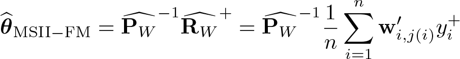
3. Rerun MSII using the modified matched sample $S^{+}={\left\{\left(y_i^{+},x_{1i},\overline{x_{2j(i)}},z_i\right)\right\}}_{i=1}^n$ to obtain the final estimator

${\widehat{\theta }}_{\text{MSII}-\text{FM}}={\widehat{P_W}}^{-1}{\widehat{R_W}}^{+}={\widehat{P_W}}^{-1}\frac{1}{n}{\displaystyle \sum _{i=1}^n{w}_{i,j(i)}^{\prime }}{y}_i^{+}$

Theorem 3 (Hirukawa and Prokhorov [2018], theorem 4). Under some regularity conditions, as n, m → ∞,

$\{\begin{array}{ll}\sqrt{n}\left({\widehat{\theta }}_{\text{MSII}-\text{FM}}-\theta \right)\stackrel{d}{\to }N\left(0,V_I\right)\hfill & if n/m\to \kappa \in (0,\infty )\text{ and }{d}_3=2,3\hfill \\ \sqrt{n}\left({\widehat{\theta }}_{\text{MSII}-\text{FM}}-\theta \right)\stackrel{d}{\to }N\left(0,V_{II}\right)\hfill & if n/m\to 0\text{ and }{d}_3=3,4\hfill \\ \sqrt{m}\left({\widehat{\theta }}_{\text{MSII}-\text{FM}}-\theta \right)\stackrel{d}{\to }N\left(0,V_{III}\right)\hfill & if n/m\to \infty \text{ and }{d}_3=2,3\hfill \end{array}$

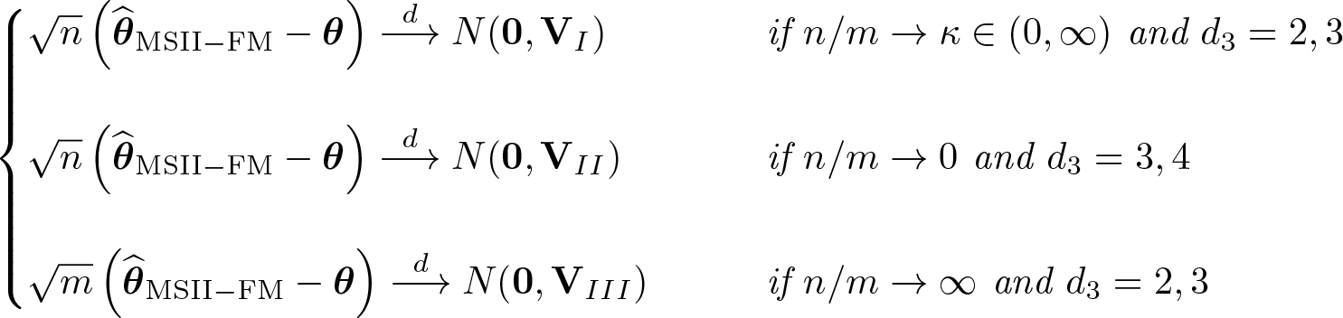
where the definitions of V _I, V _II, and V _III are the same as in theorem 2.

In practice, the standard errors (SEs) resulting from each of the three cases may be quite different. The relative magnitudes of n and m determine which case applies. Hirukawa and Prokhorov (2018) did not provide any generic comparisons for the variance matrices. Besides the scaling factor, the differences can be attributed to the specific features of the datasets and model specification. In borderline cases, it is advisable to use larger SEs for conservative inference.

3 The msreg command

3.1 Syntax

msreg has the following syntax.

msreg depvar [ varlist_X1 ] ( varlist_X2 = varlist_Z ) using filename [ if ] [ in ]

[ , vce( vce spec ) estimator( est spec ) nneighbor( # ) metric( metric spec )

order( # ) noconstant level( # ) display_options coeflegend ]

3.2 Options

vce( vce_spec ) specifies the type of variance–covariance matrix used in computation. vce_spec can be one of vi, vii, or viii. The default is vce(vi). The definition of vi, vii, and viii can be found in theorem 2.

estimator( est_spec ) specifies the type of estimator. est_spec can be either onestep or twostep. onestep specifies to use the one-step bias-corrected estimator. twostep specifies to use the two-step bias-corrected estimator. The default is estimator(twostep). ¹

nneighbor( # ) specifies the number of matches per observation. The default is nneighbor(1). The maximum allowed number of matches is 10. Each observation is matched with the mean of the specified number of observations from the other dataset.

metric( metric_spec ) specifies the distance matrix that is used as the weight matrix in a quadratic form that transforms the multiple distances into a single distance measure. metric_spec can be either mahalanobis or euclidean. metric(mahalanobis) specifies to use the inverse of the sample covariance matrix of matching variables, which is the default. metric(euclidean) specifies to use the inverse of only diagonal elements of the sample covariance matrix of matching variables.

order( # ) specifies the order of polynomials in the power-series approximation for MSII-FM. The default is order(2). The maximum allowed number of order is 5.

noconstant suppresses the constant term.

level( # ) specifies the level of significance for the output table.

display_options: noci, nopvalues, noomitted, vsquish, noemptycells, baselevels, allbaselevels, nofvlabel, fvwrap( # ), fvwrapon(style), cformat( %fmt ), pformat(% fmt ), sformat(% fmt ), and nolstretch; see [R] Estimation options.

coeflegend specifies that the legend of the coefficients and how to specify them in an expression be displayed rather than displaying the statistics for the coefficients.

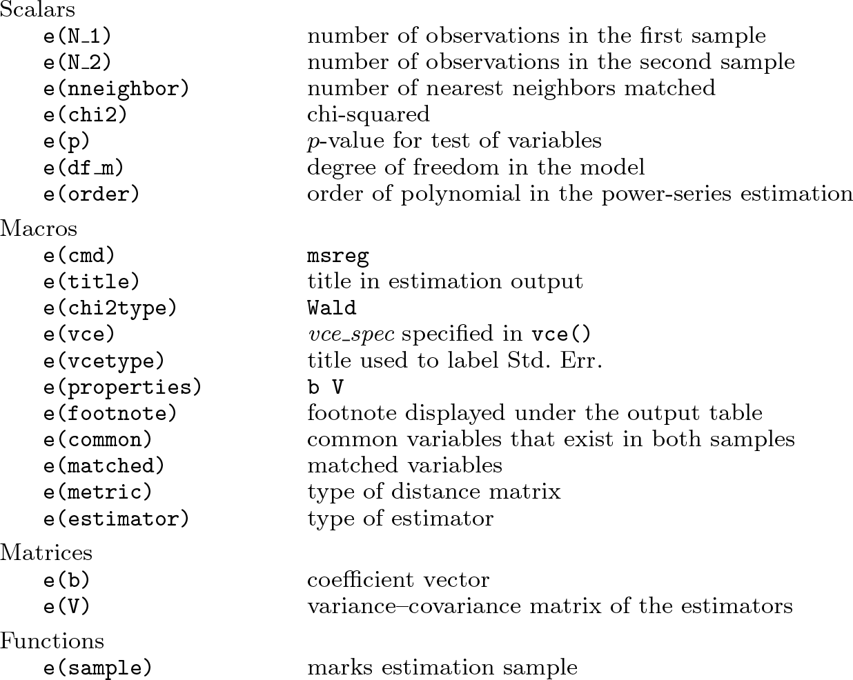
3.3 Stored results

msreg stores the following in e():

3.4 A numerical example

We illustrate the use of msreg with a numerical example.

For illustration, we simulate two datasets: s1.dta and s2.dta. The first sample, s1.dta, contains the dependent variable y and some independent variables, x11, x12, z1, and z2. The second sample, s2.dta, contains some other dependent variables x21, x22, z1, and z2. Notice that variables z1 and z2 exist in both samples. In contrast, the variables x21 and x22 exist only in the second sample, s2.dta. The data-generating process is described in section 4.

We want to fit the following regression model:

$y={\beta }_0+{\beta }_{11}{x}_{11}+{\beta }_{12}{x}_{12}+{\beta }_{21}{x}_{21}+{\beta }_{22}{x}_{22}+{\gamma }_1{z}_1+{\gamma }_2{z}_2+u$

1

The true values of all the coefficients are set to 1.

Apparently, we cannot estimate (1) using just the first sample, s1.dta, because the variables x21 and x22 are missing in this dataset. Instead, we want to use the common variables that exist in both samples, that is, z1 and z2, to construct matched variables x22 and x21 from the second sample, s2.dta.

We now use msreg to estimate the coefficients in (1). We can use the default two-step bias-corrected estimator and the default vi type variance if we assume n/m converges to a nonzero constant.

Here are some comments on the syntax.

The (x21 x22 = z1 z2) specifies that the variables x21 and x22 are the variables to be matched, and the variables z1 and z2 are the common variables that exist in both samples.

using s2 specifies that the variables x21 and x22 come from s2.dta.

We use the default two-step bias-corrected estimator.

The default option vce(vi) specifies to use the vi-type variance matrix as specified in theorem 2 because we assume the sample-size ratio between the two samples converges to a nonzero constant and there are only two continuous common variables used for matching. Actually, the note states a similar explanation about vce(vi).

Option nneighbor(2) specifies to pick out 2 matches via the NNM.

Option order(3) specifies to fit a third-order polynomial in the power-series approximation for MSII-FM.

The output shows the point estimates of coefficients and their SEs, and they can be interpreted as in a regular linear regression framework.

4 A simulation study

4.1 Simulation design

We conduct a Monte Carlo simulation study for two purposes: first, we want to see the finite-sample performance of MSII-FM in contrast to MSOLS; second, the simulation results can serve as a verification of the numerical implementation of our command msreg. The simulation study replicates that of Hirukawa and Prokhorov (2018).

The model considered throughout is

$y={\beta }_0+x_1^{\prime }{\beta }_1+x_2^{\prime }{\beta }_2+z^{\prime }\gamma +u$

2

where x ₁ = (x ₁₁ , x ₁₂) ^′ , β ₁ = (β ₁₁ , β ₁₂) ^′ ∊ R ², x ₂ = (x ₂₁ , x ₂₂) ^′ , β ₂ = (β ₂₁ , β ₂₂) ^′ ∊ R ², and $z={\left(z_1,\dots ,z_{d_3}\right)}^{\prime },$ $\gamma ={\left({\gamma }_1,\dots ,{\gamma }_{d_3}\right)}^{\prime }\in R^{d_3}$ for d ₃ = 1, 2, 3. We assume that two samples, namely, $S_1={\left\{\left(y_i,x_{1i},z_i\right)\right\}}_{i=1}^n$ and $S_2={\left\{\left(x_{2j},z_j\right)\right\}}_{j=1}^m$ are observable in practice.

Here is how to generate the data. First, $z^{\ast }=\left(z_1^{\ast },z_2^{\ast },z_3^{\ast }\right)$ is generated by

$z^{\ast }\stackrel{\text{ i.i.d. }}{\sim }N\left(\left[\begin{array}{l}0\hfill \\ 0\hfill \\ 0\hfill \end{array}\right],\hspace{0.17em}\hspace{0.17em}\left[\begin{array}{ccc}1& 1/\sqrt{2}& 1/\sqrt{3}\\ 1/\sqrt{2}& 1& \sqrt{2}/\sqrt{3}\\ 1/\sqrt{3}& \sqrt{2}/\sqrt{3}& 1\end{array}\right]\right)$

Each $z_p^{\ast }(p=1,2,3)$ is transformed to $z_p=4\Phi \left(z_p^{\ast }\right)-2$ , where Φ(·) is the cdf of N(0, 1). Notice that z_p are mutually correlated U[−2, 2] random variables. For a given d ₃, the z_p (p ≤ d ₃) are used as matching variables.

Second, x ₁ = (x ₁₁ , x ₁₂) ^′ is generated by $x_{1q}={\displaystyle {\sum }_{p=1}^{d_3}{z}_p+{\eta }_q(q=1,2)}$ , where ηq ∼ N(0, 1). Third, x ₂ = (x ₂₁ , x ₂₂) ^′ is generated by $x_{2r}={\displaystyle {\sum }_{p=1}^{d_3}{g}_{2r}\left(z_p\right)+{\eta }_{2r}}$ (r = 1, 2) for some nonlinear function g _{2 r} (·), where η _{2 r} ∼ N(0, 1). Specifically, g ₂₁(z) = z + (5/τ) ϕ(z/τ), τ = 0.25, where ϕ(·) is the pdf of N(0, 1), and $g_{22}(z)=4\sqrt{|z/2|(1-|z/2|)}\sin \{2\text{π}(1+ϵ)/(|z/2|+ϵ)\}$ , with ⲉ = 0.05.

Finally, y is generated by setting all coefficients equal to 1 with $u\stackrel{\text{ i.i.d. }}{~}N(0,1)$ . The sample sizes are set to (n, m) = (1000, 1000). The number of replications is 1,000.

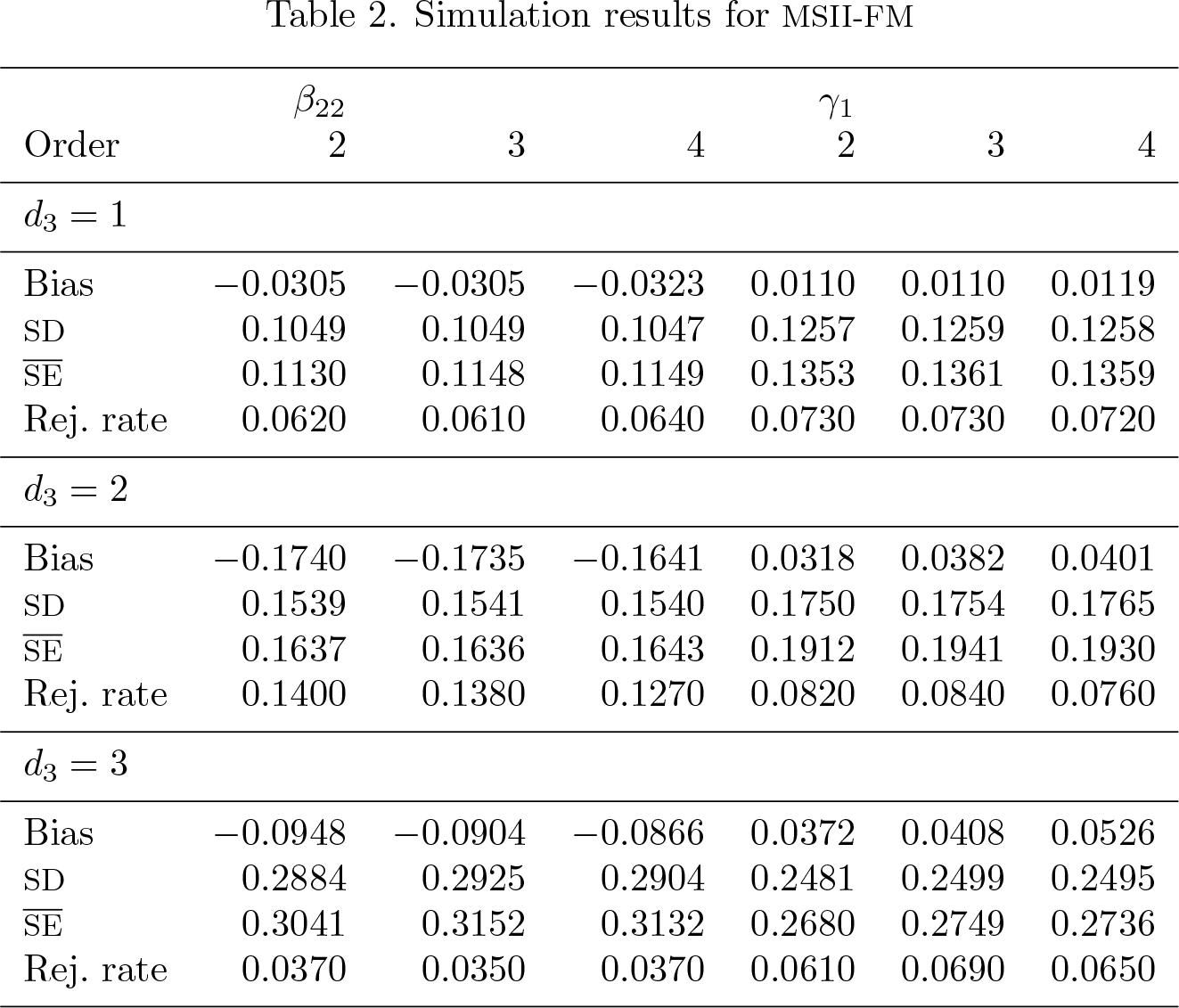
We focus on the finite-sample properties of estimators of β ₂₂ and γ ₁. For each estimator, the following performance measures are computed: i) Bias (1−Mean), where Mean is the simulation average of the parameter estimate; ii) standard deviation (SD) (simulation SD of the parameter estimate); iii) $\overline{\text{SE}}$ (simulation average of the SE); and iv) Rej. rate (rejection rate for the test of parameter estimate equal to its true value 1 against the nominal 5% level of significance).

For d ₃ = 1, 2, 3, we estimate the coefficients in (2) using both MSOLS and MSII-FM. For MSOLS, the number of matches is K = 1, 2, 4, 8. For MSII-FM, the number of matches K is fixed at 1, and orders of polynomials in the power-series approximation are 2, 3, and 4. For a more complete simulation study, see section 4 of Hirukawa and Prokhorov (2018).

4.2 Results

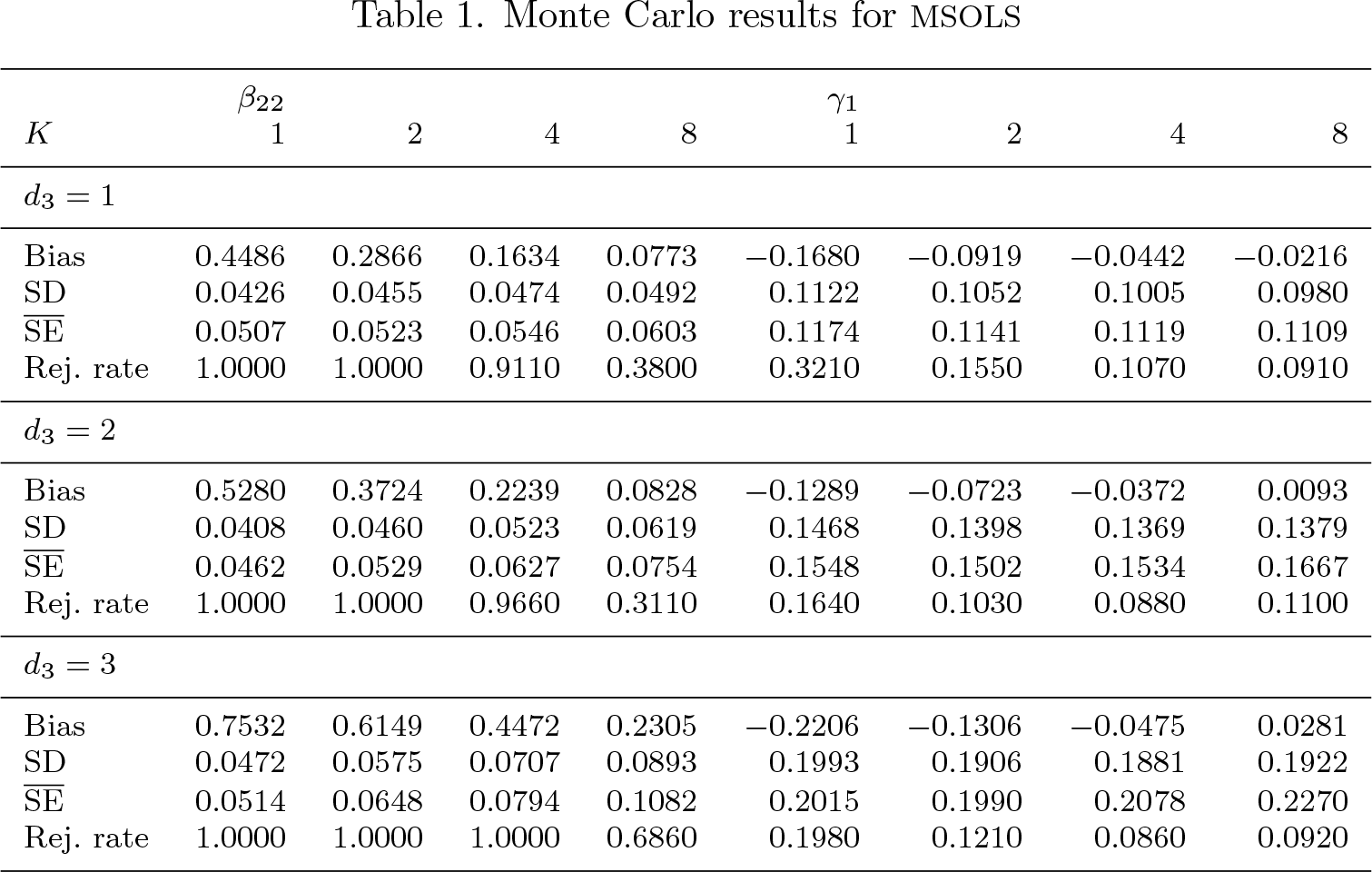
The simulation results are summarized in tables 1 and 2 for MSOLS and MSII-FM, respectively.

Table 1 shows that regardless of the number of matches, there is a big bias of β ₂₂, and there is a large rejection rate, which indicate inconsistency of MSOLS as implied in theorem 1.

Table 1.

Monte Carlo results for MSOLS

	β 22				γ 1
K	1	2	4	8	1	2	4	8
d 3 = 1
Bias	0.4486	0.2866	0.1634	0.0773	−0.1680	−0.0919	−0.0442	−0.0216
SD	0.0426	0.0455	0.0474	0.0492	0.1122	0.1052	0.1005	0.0980
$\overline{\text{SE}}$	0.0507	0.0523	0.0546	0.0603	0.1174	0.1141	0.1119	0.1109
Rej. rate	1.0000	1.0000	0.9110	0.3800	0.3210	0.1550	0.1070	0.0910
d 3 = 2
Bias	0.5280	0.3724	0.2239	0.0828	−0.1289	−0.0723	−0.0372	0.0093
SD	0.0408	0.0460	0.0523	0.0619	0.1468	0.1398	0.1369	0.1379
$\overline{\text{SE}}$	0.0462	0.0529	0.0627	0.0754	0.1548	0.1502	0.1534	0.1667
Rej. rate	1.0000	1.0000	0.9660	0.3110	0.1640	0.1030	0.0880	0.1100
d 3 = 3
Bias	0.7532	0.6149	0.4472	0.2305	−0.2206	−0.1306	−0.0475	0.0281
SD	0.0472	0.0575	0.0707	0.0893	0.1993	0.1906	0.1881	0.1922
$\overline{\text{SE}}$	0.0514	0.0648	0.0794	0.1082	0.2015	0.1990	0.2078	0.2270
Rej. rate	1.0000	1.0000	1.0000	0.6860	0.1980	0.1210	0.0860	0.0920

Table 2 shows that 1) the bias is small; that is, the mean of the point estimates is very close to its true value; 2) the SD of the point estimate is very close to the mean of the SEs; and 3) the overall rejection rate is close to the nominal 5% level. Notice that for the case d ₃ = 2, the rejection rate is a little bit off for β ₂₂. However, based on results for larger samples, it seems that the over-rejection rate is due to the finite-sample bias of MSII-FM (reported in the Supplement of Hirukawa and Prokhorov [2018]). The simulation result shows that MSII-FM performs well in a finite sample as predicted by theorem 3 and that it also numerically verifies the implementation of msreg.

Table 2.

Simulation results for MSII-FM

	β 22			γ 1
Order	2	3	4	2	3	4
d 3 = 1
Bias	−0.0305	−0.0305	−0.0323	0.0110	0.0110	0.0119
SD	0.1049	0.1049	0.1047	0.1257	0.1259	0.1258
$\overline{\text{SE}}$	0.1130	0.1148	0.1149	0.1353	0.1361	0.1359
Rej. rate	0.0620	0.0610	0.0640	0.0730	0.0730	0.0720
d 3 = 2
Bias	−0.1740	−0.1735	−0.1641	0.0318	0.0382	0.0401
SD	0.1539	0.1541	0.1540	0.1750	0.1754	0.1765
$\overline{\text{SE}}$	0.1637	0.1636	0.1643	0.1912	0.1941	0.1930
Rej. rate	0.1400	0.1380	0.1270	0.0820	0.0840	0.0760
d 3 = 3
Bias	−0.0948	−0.0904	−0.0866	0.0372	0.0408	0.0526
SD	0.2884	0.2925	0.2904	0.2481	0.2499	0.2495
$\overline{\text{SE}}$	0.3041	0.3152	0.3132	0.2680	0.2749	0.2736
Rej. rate	0.0370	0.0350	0.0370	0.0610	0.0690	0.0650

5 An empirical application: Return to schooling

We now apply msreg to a version of Mincer’s (1974) wage equation. We consider the following wage regression,

$\begin{array}{c}\log (\text{wage })={\beta }_0+{\beta }_1\text{expr}+{\beta }_2{\text{expr}}^2+{\beta }_3\text{kww}+{\beta }_4\text{educ}+{\beta }_5\text{feduc}+{\beta }_6\text{meduc}\\ +{\beta }_7\text{smsa}+{\beta }_8\text{south}+{\beta }_9\text{black}+u\end{array}$

3

where expr is years of experience, educ is years of education, kww is Knowledge of World of Work test score, feduc and meduc are years of father’s and mother’s education, and black, smsa, and south are dummy variables to indicate whether an individual is black, lives in an urban area, and lives in the south, respectively.

We can estimate (3) using only card.dta from Card (1995), as in the benchmark OLS result below.

The estimation result is stored as ols.

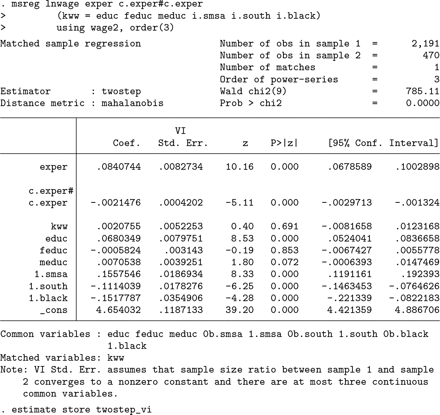
Nonetheless, we pretend that the variable kww is missing in this dataset. In accordance with this scenario, we use yet another dataset, wage2.dta, from Blackburn and Neumark (1992). The dataset contains six variables—educ, feduc, meduc, smsa, south, and black—other than kww. All six variables are used as matching variables to impute the missing kww, where educ, feduc, and meduc are assumed to be continuous. Our aim is to see how the estimation result of (3) changes if kww is imputed from wage2.dta.

We use the default vi type covariance estimation assuming the sample-size ratio between the two datasets converge to a nonzero constant. We use a third-order polynomial in power-series estimation to remove the second-order bias. The estimation result is stored as twostep_vi.

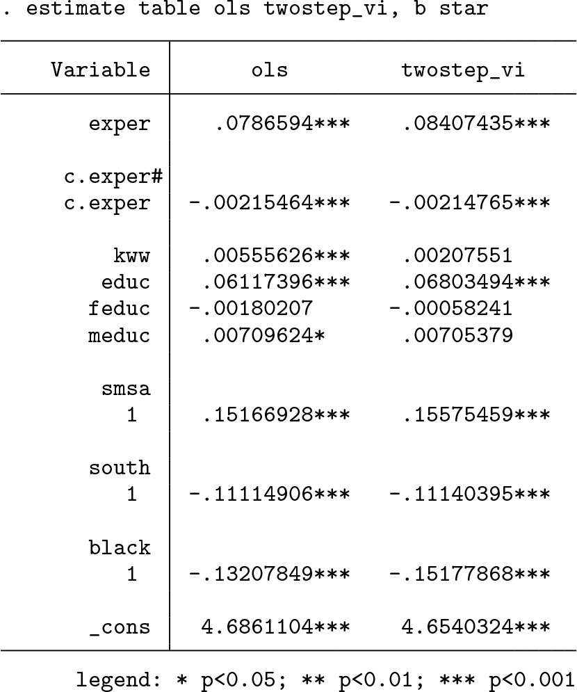
We can now compare these two estimation results.

The first column shows the benchmark OLS results. The signs of expr, expr ², kww, and educ are as expected, and the estimates are significant at the 5% level.

The second column shows the results from the two-step bias-corrected estimator with the default vi-type covariance. All the point estimates have the same sign as in the OLS benchmark. However, the coefficient on kww is insignificant because of a large SE.

6 Conclusion

In this article, we described a new command, msreg, that implements two estimators proposed in Hirukawa and Prokhorov (2018). The command allows users to obtain consistent estimators of linear regression models after imputing missing regressors via the NNM. We illustrated the use of msreg through a numerical example and an empirical application.

Supplemental Material

Supplemental Material, sj-zip-1-stj-10.1177_1536867X211000008 - msreg: A command for consistent estimation of linear regression models using matched data

Supplemental Material, sj-zip-1-stj-10.1177_1536867X211000008 for msreg: A command for consistent estimation of linear regression models using matched data by Masayuki Hirukawa, Di Liu and Artem Prokhorov in The Stata Journal