Bootstrap unit-root test for random walk with drift: The bsrwalkdrift command

Abstract

In this article, we introduce the command bsrwalkdrift, which is primarily intended to perform a bootstrap unit-root test under the null hypothesis of random walk with drift. The method implemented in this command is considerably more precise than the corresponding case of the conventional augmented Dickey–Fuller test, which can be inaccurate when the true value of the drift term is small relative to the standard deviation of the innovations. The command also has an option to account for deterministic linear trend and another option to perform bootstrap unit-root tests under the null hypothesis of random walk without drift.

1 Introduction

One particular case of the augmented Dickey–Fuller (ADF) test is when the null hypothesis is that the data-generation process (DGP) corresponds to a random walk with a nonzero drift. For this case, Hamilton (1994, 495–497) proves that the asymptotic distribution for the test statistic is standard normal. So he suggested that the standard ordinary least-squares (OLS) t and F statistics can be compared with the standard t and F distribution when performing the test on finite samples (see Hamilton [1994, 497]). This method is implemented in the dfuller command by specifying the option drift. ¹

Although the t distribution can be a good approximation for large enough samples, it is rather inaccurate for small or even medium sample sizes, especially when the true value of the drift term is small relative to the standard deviation of the innovations. For example, our simulations with the dfuller, drift command, with a drift term of 0.1, a standard deviation of 1, a sample size of 100 observations, and 2,000 simulation replicates, produced a mean rejection rate of 0.360. That rate looks too far from the nominal rejection probability of 0.05. When we increased the drift term to 0.25 and the sample size to 200, the mean rejection rate was 0.132, which still does not seem near enough to 0.05. This issue was previously investigated by Hylleberg and Mizon (1989).

To overcome the problem above, we wrote the bsrwalkdrift command, which uses a bootstrapping technique based on the method proposed by Park (2003). He considers the ADF unit-root tests for autoregressive unit-root models. According to Park (2003), testing with bootstrap critical values is expected to correct for the discrepancy between the finite sample and nominal rejection rates. He performed simulations that showed rejection probabilities close to their nominal values. Although his method was originally defined under the null hypothesis of random walk without drift, he also states, “It can be clearly seen that our methodology may also be used to analyze many other unit root tests as well.” In this sense, we use a straightforward adaptation for the null hypothesis of a random walk with drift.

Although we primarily wrote bsrwalkdrift to correct for the issue described above, we also included an option to account for deterministic linear trend and another option to test the hypothesis of random walk without drift. They allow for testing strategies that require analyzing more than one case, and they are expected to have better finite sampling properties under particular situations that can affect the conventional ADF tests (for example, DGP with nonnormal innovations).

The remainder of the article is organized as follows. Section 2 describes the method implemented in the command. Section 3 presents the syntax for bsrwalkdrift and includes an example to illustrate the use of the command. Section 4 presents the simulation results to evaluate the performance of the bsrwalkdrift command compared with the dfuller, drift command. Section 5 concludes.

2 The method

The method to compute the bootstrap critical value for the unit-root test is based on Park (2003). We test the null hypothesis

$H_0:\delta =0$

in the model

$\text{Δ}{y}_t=\alpha +\delta y_{t-1}+{\displaystyle \sum _{i=1}^p{\beta }_i\text{Δ}{y}_{t-i}+{ϵ}_t}$

1

where ⲉ_t is an independent and identically distributed sequence such that E(ⲉ_t ) = 0 and E(|ⲉ_t|^r ) < ∞ for r > 1.

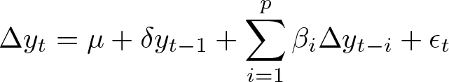
We begin by fitting the regression

$\text{Δ}{y}_t=\alpha +{\displaystyle \sum _{i=1}^p{\beta }_i\text{Δ}{y}_{t-i}+{ϵ}_t}$

2

on a series defined as (y _{− p},…, y ₀ , y ₁ ,…, y_T ). According to Park (2003), the resampling should be performed from the restricted model (2) instead of the unrestricted model (1). For more details on this, see Basawa et al. (1991).

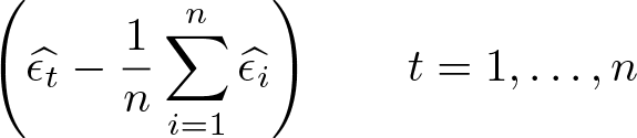
Then, we compute the estimated residuals $\left({\widehat{ϵ}}_t\right)$ , draw bootstrap samples, and obtain demeaned residuals

$\left({\widehat{ϵ}}_t-\frac{1}{n}{\displaystyle \sum _{i=1}^n{\widehat{ϵ}}_i}\right)\hspace{1em}t=1,\dots ,n$

denoting them by $\left({\widetilde{ϵ}}_t\right)$ . Notice that without demeaning, the mean of the bootstrap sample would not be zero.

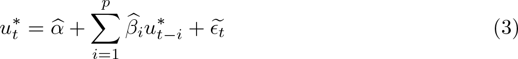
For each bootstrap sample $\left({\widetilde{ϵ}}_t\right)$ , we generate $\left(u_t^{\ast }\right)$ recursively from $\left({\widetilde{ϵ}}_t\right)$ using

$u_t^{\ast }=\widehat{\alpha }+{\displaystyle \sum _{i=1}^p{\widehat{\beta }}_i{u}_{t-i}^{\ast }+{\widetilde{ϵ}}_t}$

3

starting from (u _{− p +1} ,…, u ₀). Next, we generate the bootstrap samples $\left(y_t^{\ast }\right)$ from y ₀ through

$y_t^{\ast }=y_0+{\displaystyle \sum _{i=1}^t{u}_{t-i}^{\ast }}$

4

The initializations for (3) and (4) are obtained by fixing (y _{− p},…, y ₀) and using u_t = Δy_t to calculate (u _{− p +1} ,…, u ₀). According to Park (2003), the initializations are important to make his theory applicable; however, they are irrelevant for the models with constant and deterministic trend.

For each bootstrap sample $\left(y_t^{\ast }\right)$ , we fit regressions

$\text{Δ}{y}_t^{\ast }={\alpha }^{\ast }+{\delta }^{\ast }{y}_{t-1}^{\ast }+{\displaystyle \sum _{i=1}^p{\beta }_i^{\ast }\text{Δ}{y}_{t-i}^{\ast }+v_t}$

and collect the t statistics for δ ^∗. The set of those values constitutes a bootstrap approximation to the null distribution of the t statistic. Therefore, given a significance level of λ, the bootstrap critical value for the test is the corresponding λ×100th percentile.

Finally, we fit the regression

$\text{Δ}{y}_t=\mu +\delta y_{t-1}+{\displaystyle \sum _{i=1}^p{\beta }_i\text{Δ}{y}_{t-i}+{ϵ}_t}$

on the original sample and compute the t statistic associated with δ, which is to be compared with the bootstrap critical value described above. If the t statistic is less than the bootstrap critical value, we reject the hypothesis that there is a unit root. In addition, we compute the p-value as the proportion of the number of values, from the bootstrap approximation to the null distribution, that is less than the t statistic.

2.1 Model with deterministic linear trend

Trending time series could be stationary around a deterministic trend, or the trending behavior could be stochastic. For trending series, the first step of the analysis should be testing for unit root, accounting for a possible deterministic trend. If the series is actually stationary around a deterministic trend, unit-root testing using models without trend is expected to have no power (Campbell and Perron 1991).

Park (2003) dedicated a section of his article to models with deterministic trends. He proposed to first detrend the series and then apply his bootstrapping algorithm to the detrended series. In the case of linear trend, the detrended series may be obtained by fitting the OLS regression

$y_t={\widehat{\beta }}_0+{\widehat{\beta }}_{1}t+y_t^d$

and using the residuals $y_t^d$ as the detrended series. In this case, the alternative hypothesis is that the original series is stationary around a deterministic linear trend.

Park (2003) provided analytical proof that testing on a detrended series and the ADF test with trend are asymptotically equivalent not only in the first order but also in the second order.

3 The command bsrwalkdrift

3.1 The command

Syntax

The command syntax is

bsrwalkdrift varname [ if ] [ in ] [ , lags( # ) bsreps( # ) siglevel( # )

seed( # ) nodrift detrend selecic( stat ) maxlag( # ) plot nodots ]

The data must be tsset before using the command.

Options

lags( # ) specifies the number of lagged differences. The default is lags(1).

bsreps( # ) specifies the number of bootstrap replicates. The default is bsreps(500).

siglevel( # ) specifies the significance level for the test. The default is siglevel(0.05).

seed( # ) specifies the random-number seed.

nodrift specifies that the DGP is a random walk without drift for the null hypothesis. ²

detrend detrends the series assuming a linear trend and performs the test on the detrended series. If this option is specified, the command automatically activates the nodrift option.

selecic( stat ) specifies that the lag order be selected by minimizing information criteria. maxlag( # ) is required if selecic( stat ) is specified. selecic(aic) specifies the Akaike information criterion (aic). selecic(bic) specifies the Bayesian information criterion (bic). selecic( stat ) fits a sequence of regressions using (2) for p = 0, 1, 2,…, P on a common estimation sample, which is the sample for p = P . The AIC or BIC is computed for each regression, and the selected lag order corresponds to the minimum value. P is set by maxlag( # ).

maxlag( # ) sets the maximum lag order to #. This option is required if selecic( stat ) is specified. # must be greater than 1 and less than a third of the sample size.

plot creates a kernel density plot of the bootstrap null distribution.

nodots suppresses replication dots.

Stored results

bsrwalkdrift stores the following in r():

3.2 Example

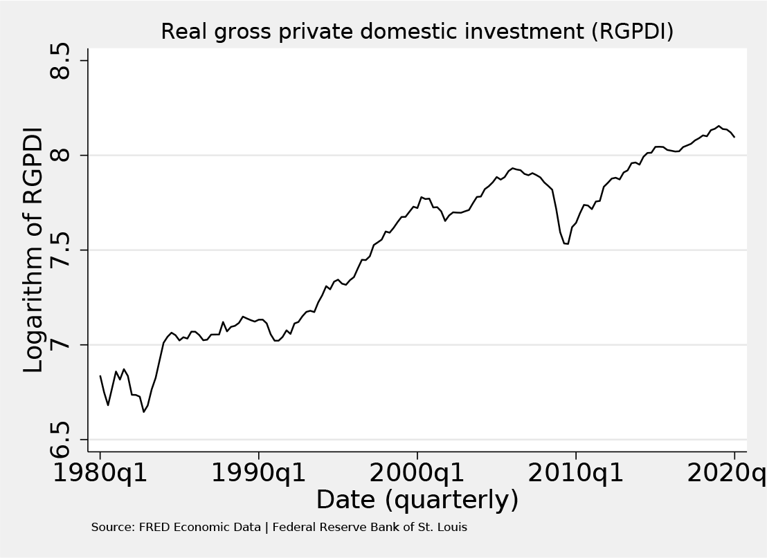
We analyze a quarterly series for real gross private domestic investment in the United States for the period from 1980q1 to 2020q1. ³ In figure 1, we plot the natural logarithm of real gross private domestic investment (variable ln_rgpdinv). As can be seen, the series has a clear upward trend. It does not seem clear, however, whether the trend is deterministic or stochastic. To clarify the doubt, our testing strategy begins by performing the bootstrap unit-root test on the detrended series by specifying the detrend option. If we reject the null hypothesis of random walk, it would be evidence that the series is stationary around a deterministic linear trend. If instead we fail to reject the null hypothesis, the trend would likely be stochastic; more specifically, the series would be a random walk with drift. This is precisely the default case for the bsrwalkdrift command, and so we can use it to confirm that.

Figure 1.

Natural logarithm of real gross private domestic investment

We begin by using bsrwalkdrift with the detrend option to test that ln_rgpdinv is a random-walk process against the alternative that the series is stationary around a linear trend. We tell the command to select the lag order using the aic. To do so, we specify the options selecic(aic) and maxlag(8). We also specify 5,000 bootstrap replicates, keep the default 0.05 significance level, and specify some other options as well.

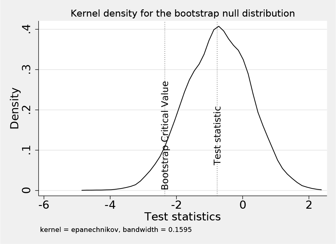
bsrwalkdrift issues an explanatory note associated with the detrend option (see the output). After that, the command reports a table with the AIC up to lag 8 followed by the selected lag order, which is lag 4 in this case. Then, it follows the OLS auxiliary regression for the detrended series. After that, the command reports the results of the bootstrap testing method. The most important results are the test statistic, which is taken from the OLS auxiliary regression; the bootstrap critical value; and the p-value based on the bootstrap null distribution. Because the value of the test statistic (−2.3582) is larger than the bootstrap critical value (−3.0084), the null hypothesis cannot be rejected. The p-value (0.2228) leads to the same conclusion, which will always be the case if compared with the specified significance level. Hence, we can rule out that the series is stationary around a linear trend. Because the plot option was specified, the command creates a kernel density plot of the bootstrap null distribution, with vertical dotted lines representing the bootstrap critical value and the test statistic (see figure 2).

Figure 2.

Kernel density plot of the bootstrap null distribution for the detrended series

So far, the evidence is against stationarity around a linear trend and in favor of stochastic trend. Thus, we now use the default case of bsrwalkdrift (random walk with drift); and so, we just remove the detrend option and maintain the other options previously specified.

The selected lag order was again lag 4. The test statistic (−0.7695) is larger than the bootstrap critical value (−2.3527), which must be consistent with the p-value (0.4816); therefore, the null hypothesis of random walk with drift cannot be rejected. This result with the detrended case indicates that the series is actually a random walk with drift. Figure 3 is the plot of the corresponding kernel density for the bootstrap null distribution.

Figure 3.

Kernel density plot of the bootstrap null distribution

4 Simulations

We evaluated some finite-sample properties of bsrwalkdrift by performing Monte Carlo simulations.

The model is

$y_t=\alpha +y_{t-1}+{\beta }_1\text{Δ}{y}_{t-1}+{\beta }_2\text{Δ}{y}_{t-2}+e_t$

where

$\begin{array}{l}{e}_t\sim N(0,1)\hfill \\ {\beta }_1=0.5\hfill \\ {\beta }_2=-0.2\hfill \\ \alpha =0.05,\hspace{0.17em}0.1,\hspace{0.17em}0.25,\hspace{0.17em}0.5,\text{ and }\hspace{0.17em}0.75\hfill \\ \text{nobs }=25,\hspace{0.17em}50,\hspace{0.17em}100,\hspace{0.17em}200,\text{ and }\hspace{0.17em}500\hfill \end{array}$

For each combination of α and nobs (sample size), we generated the data for y with the model above, and we used

for 2,000 simulation replicates, where bsrwalkdrift uses 200 bootstrap replicates for each simulation replicate. The rejection results were stored for all the replicates, and then we estimated the mean rejection rates for a 0.05 significance level.

Below, we used the tabdisp command to create a table with the simulation results. rejrate is the mean rejection rate for dfuller, drift, and bsrejrate is the mean rejection rate of bsrwalkdrift. llbsrrate and ulbsrrate are the lower and upper limits, respectively, of the 95% confidence intervals for bsrejrate.

The output shows that rejrate tends to be farther from the nominal rate (0.05) because both the value of alpha (the drift term) and the number of observations are smaller. On the other hand, bsrejrate is always nicely near the nominal rate. Also, notice that in all the cases, the confidence intervals cover the nominal rate.

5 Conclusion

The mean rejection rates from our simulations showed that bsrwalkdrift provides a correction for the ADF test that is particularly relevant with small or medium sample sizes and a small or medium drift term. Therefore, this command would be a recommendable alternative to perform unit-root testing for the null hypothesis that the process is a random walk with a drift. Finally, the command has an option to test for random walk appropriate for trending series, and there is another option to test for random walk without drift, which would be appropriate for series with no apparent trend.

Supplemental Material

Supplemental Material, sj-zip-1-stj-10.1177_1536867X211000003 - Bootstrap unit-root test for random walk with drift: The bsrwalkdrift command

Supplemental Material, sj-zip-1-stj-10.1177_1536867X211000003 for Bootstrap unit-root test for random walk with drift: The bsrwalkdrift command by Miguel Dorta and Gustavo Sanchez in The Stata Journal