
Abstract
In cross-sectional time-series data with a dichotomous dependent variable, failing to account for duration dependence when it exists can lead to faulty inferences. A common solution is to include duration dummies, polynomials, or splines to proxy for duration dependence. Because creating these is not easy for the common practitioner, I introduce a new command,
1 Introduction
It is well known that when one models a dichotomous dependent variable in binary cross- sectional time-series data (B-CSTS), failing to account for duration dependence—the phenomenon by which the occurrence of an event at time t in unit i may make the reoccurrence of an event at a future time point more or less likely—can have severe consequences for estimation (Beck, Katz, and Tucker 1998). At best, failing to model such dependence may induce serial autocorrelation, leading to standard errors that are anticonservative. At worst, it can produce omitted variable bias even if the included regressors are unrelated to the omitted duration dependence.
A common approach recommended by Beck, Katz, and Tucker (1998) when dealing with B-CSTS data—when the occurrence of events is relatively rare—is to estimate a logistic regression (LR) with duration dummies to proxy for any duration dependence.
1
While alternative approaches exist (cf. Zorn [2000]; Box-Steffensmeier and Jones [2004]; or fitting random-effects parametric survival models using the
In this article, I introduce
2 Duration dependence with B-CSTS
Consider a simple B-CSTS dataset in long form, like the one shown in table 1. yit is a dichotomous dependent variable for unit i observed at time t that does not occur relatively often. 3 This is commonly modeled using a generalized linear model with a logit link to account for the dichotomous nature of the dependent variable (Beck, Katz, and Tucker 1998). The problem that arises is with duration dependence, which exists if the Pr(yit ) = 1 changes based on how long it has been since the last event (or entry into the sample). This is shown by the duration variable in table 1, which records the time since the last event in the data. 4
Durations in B-CSTS data
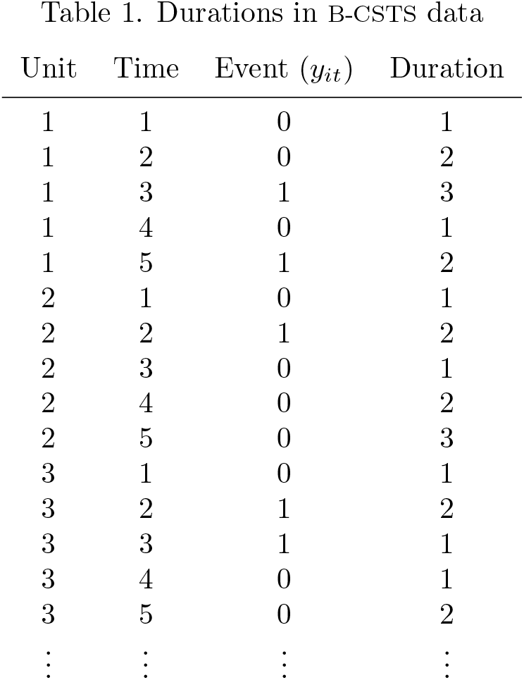
Failing to model duration dependence implies a constant hazard rate, meaning that the probability of event reoccurrence does not change over time. In other words, events are independent from one another. In real-world data, however, such an assumption is probably almost always violated. For instance, duration dependence has been argued to exist in topics as varied as conflict onsets (Clare 2010; Bapat and Zeigler 2016), pursuit of nuclear weapons (Way and Weeks 2014), and firm-level bankruptcies (Hillegeist et al. 2004). Failing to model duration dependence when it exists can lead to many problems. At best, the estimator will be inefficient, and the standard errors will be incorrect; at worst, biased and inconsistent estimates may result because failing to include duration when it exists is a form of omitted variable bias (Beck, Katz, and Tucker 1998).
Beck, Katz, and Tucker (1998) note that a straightforward way to continue to model B-CSTS data in the logit framework—but also account for duration dependence—is to simply create a time-since-last-event variable (that is, the duration variable shown in table 1), which is then turned into a vector of dummy variables. These are then included in the logit generalized linear model 5

Now, in addition to the standard covariates (
Duration dummy variables

Because it is likely that some κit may be perfectly collinear with yit , separation is likely to lead to estimation issues when using maximum likelihood; this will force Stata to drop any collinear dummy variables. To alleviate this, Carter and Signorino (2010) advocate for a simple approach of incorporating duration, duration squared, and duration cubed in the model instead of either splines (another approach that Beck, Katz, and Tucker [1998] recommend) or dummy variables. While some consider κit to be nuisance parameters (Beck 2010), others contend that it is important to discuss and interpret the estimated dependence function as a feature of theoretical interest (Carter and Signorino 2010; Williams 2016). 7 Regardless, both lines of reasoning agree that it is necessary to include some functional form of duration in the model to account for duration dependence.
One difficulty with implementing the advice above is that incorporating some functional form of duration dependence requires the creation of a duration variable, which is far less straightforward than taking lags or including time dummies in standard cross- sectional time-series data with a continuous dependent variable. This difficulty is compounded if some data are missing or if units enter or leave the sample at different times.
Below, I show a straightforward way to create a duration variable, even in the presence of missing data, using the command
3 Accounting for dependence with mkduration
3.1 Syntax
The command syntax is

This command requires the specification of a single variable,
3.2 Options
There are four additional options to account for various types of missing data. By default, the duration variable is created for all nonmissing values of the event variable; any gaps in the middle of the series are handled by replacing the duration variable with missings until the next event occurs.
When one specifies
4 Example
For an applied example, I use data from Philips (2020), who examines whether state governments in India time land reforms to occur just before state elections to appeal to voters. Passage of legislative land reforms is a relatively rare event, occurring in just 48 of the 515 state-years under observation, meaning that these B-CSTS data may exhibit some form of duration dependence; one intuitive expectation is that passage of reform in one year makes additional land reform passage quite unlikely in the near term.
10
To start, we will create the duration variable using the dependent variable,

The histogram is shown in figure 1. Duration is a monotonically decreasing function with a maximum duration of 32 years, meaning that no land reform occurred during 32 years “at risk” for one of the states.
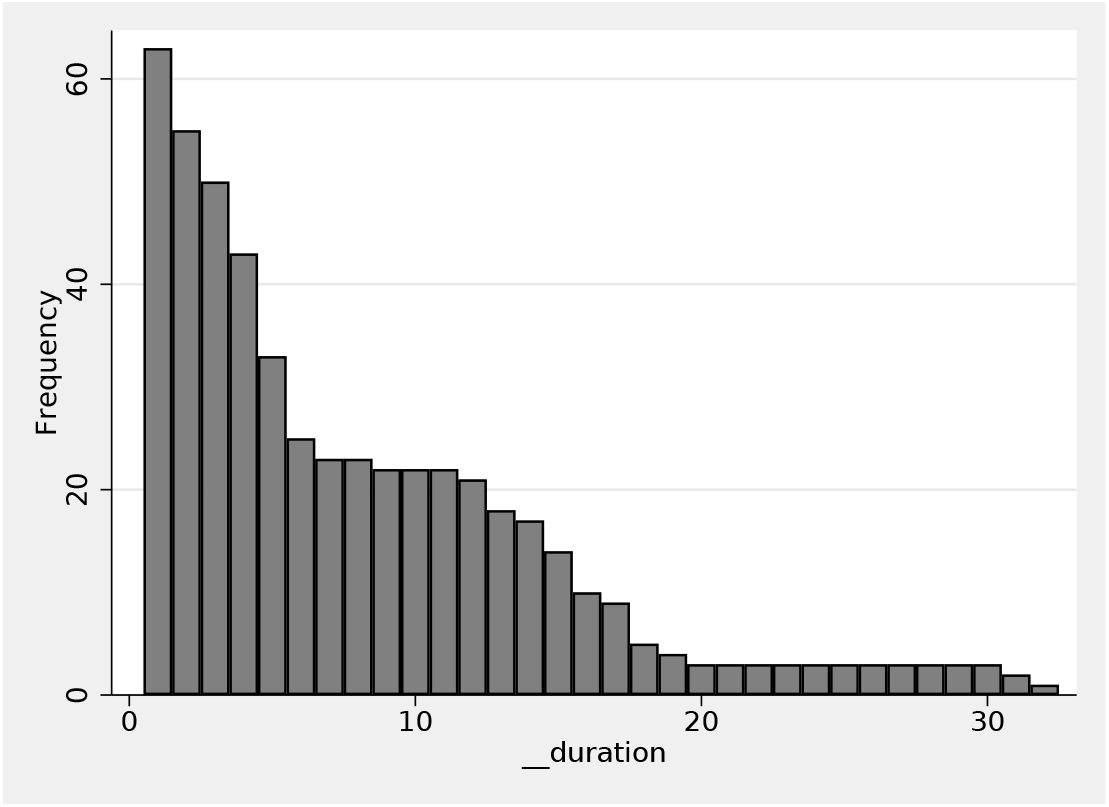
Histogram of
By default, the generated duration variable is called

The results are shown in table 3, model 1. As is clear from the table, because of perfect collinearity (no land reform ever occurs for many of the duration-years), many duration dummies fall out of the model, reducing the number of observations. For the other covariates, it appears that land reform is more likely in the year before a state legislative election. Land reform is also more likely in multiparty competitive political systems than it is for two-party or single-party competition.
Different approaches to account for duration

NOTE: Dependent variable is equal to 1 if state i enacted land reform in year t, 0 otherwise. LR-test results not available for model 1 because of sample-size difference. Random-effects LR with standard errors in parentheses. Two-tailed tests.
* p < 0.10, ** p < 0.05, *** p < 0.01.
Instead of including duration dummies, we can use the recommendation of Carter and Signorino (2010) and create a cubic polynomial term of duration using Stata’s interaction capabilities:

The results using a cubic polynomial are shown in model 2 in table 3. None of the duration coefficients are statistically significant, which suggests they may not be needed. The results remain similar to those in model 1, although multiparty government is no longer statistically significant, while two-party governments (specifically, one left party and one centrist party) are associated with an increased probability of land reform, although this effect is statistically significant only at the 10% level.
As an additional functional form choice, users can choose to model duration using splines:

Each command shows (respectively) a restricted cubic spline, using the default of five knots, and a piecewise linear spline with four knots (meaning that duration will be partitioned into quintiles). Note, too, that by specifying
Given that interpreting the various approaches to duration in table 3 is not straight- forward, we can instead plot the dummy variables, splines, and cubic polynomials to better understand the underlying nature of duration dependence in the data (Carter and Signorino 2010; Williams 2016). Here we fit each model and use

The resulting plot of these durations is shown in figure 2. The estimated duration for land reform appears to be nonmonotonic for all specifications except the cubic polynomial; the predicted probability of land reform increases through the first four or five years after a previous land reform and then tends to decline. For the dummy and spline durations, there appears to be another period about a dozen years after a previous land reform in which reform once again becomes more likely. After about 20 years after land reform passage, there is only a small probability of an additional land reform. Figure 2 also shows how the inclusion of the duration dummies—especially in the context of separation—can result in “bumpy” durations; moreover, in this example, we are unable to obtain predicted probabilities beyond κ 17 because of separation issues.

Different durations generated using
Missing data
One issue with duration dependence has to do with missing data. I discuss three types specific to B-CSTS data, using a stylized example shown in table 4. First, the event variable may be missing at the beginning of the series; for instance, in table 4, the event series is not observed for t = 1, 2. Second, data may be missing at the end of the series. In table 4, data are not observed for time points t = 17 to t = 20. Third, data could be missing during the interval in which the series is observed; the event in table 4 is not observed for the interval t = 7, 8, although prior and future values are observed.

By default,
A stricter interpretation might lead us to replace the duration with missings until the first event is actually observed because events may have occurred before the start of the sample (that is, left-censoring). Using the
If the user is comfortable assuming that no events have occurred during the unobserved middle time period t = 7, 8, he or she can use the
In addition to using the
5 Conclusion
In this article, I have introduced a new command,
Supplemental Material
Supplemental Material, st0621 - An easy way to create duration variables in binary cross-sectional time-series data
Supplemental Material, st0621 for An easy way to create duration variables in binary cross-sectional time-series data by Andrew Q. Philips in The Stata Journal
Footnotes
6 Acknowledgments
I thank the editor and an anonymous reviewer for their thoughtful comments and suggestions. Inspiration to write this program came from students in panel-data courses at CU Boulder and the IPSA-USP Summer School held in S˜ao Paulo, Brazil. Despite this, all errors and omissions are my own.
7 Programs and supplemental materials
To install a snapshot of the corresponding software files as they existed at the time of publication of this article, type
Notes
References
Supplementary Material
Please find the following supplemental material available below.
For Open Access articles published under a Creative Commons License, all supplemental material carries the same license as the article it is associated with.
For non-Open Access articles published, all supplemental material carries a non-exclusive license, and permission requests for re-use of supplemental material or any part of supplemental material shall be sent directly to the copyright owner as specified in the copyright notice associated with the article.