Analysis of regression-discontinuity designs with multiple cutoffs or multiple scores

Abstract

In this article, we introduce the Stata (and R) package rdmulti, which consists of three commands (rdmc, rdmcplot, rdms) for analyzing regression-discontinuity (RD) designs with multiple cutoffs or multiple scores. The command rdmc applies to noncumulative and cumulative multicutoff RD settings. It calculates pooled and cutoff-specific RD treatment effects and provides robust biascorrected inference procedures. Postestimation and inference is allowed. The command rdmcplot offers RD plots for multicutoff settings. Finally, the command rdms concerns multiscore settings, covering in particular cumulative cutoffs and two running variable contexts. It also calculates pooled and cutoff-specific RD treatment effects, provides robust bias-corrected inference procedures, and allows for postestimation and inference. These commands use the Stata (and R) package rdrobust for plotting, estimation, and inference. Companion R functions with the same syntax and capabilities are provided.

1 Introduction

Regression-discontinuity (RD) designs with multiple cutoffs or multiple scores are commonly encountered in empirical work in economics, education, political science, public policy, and many other disciplines. Thus, these specific settings have also received attention in the recent RD methodological literature (Papay, Willett, and Murnane [2011]; Reardon and Robinson [2012]; Wong, Steiner, and Cook [2013]; Keele and Titiunik [2015]; Keele, Titiunik, and Zubizarreta [2015]; Cattaneo et al. [2016, 2020], and references therein). In this article, we introduce the software package rdmulti, which consists of three commands (and analogous R functions) for the analysis of RD designs with multiple cutoffs or multiple scores.

The command rdmc applies to noncumulative and cumulative multicutoff RD settings, following recent work in Cattaneo et al. (2016, 2020). Specifically, it calculates pooled and cutoff-specific RD treatment effects, using local polynomial estimation and robust bias-corrected inference procedures. Postestimation and inference is allowed. The companion command rdmcplot offers RD plots for multicutoff settings. Finally, the command rdms concerns multiscore settings, covering in particular cumulative cutoffs and bivariate score contexts. It also calculates pooled and cutoff-specific RD treatment effects based on local polynomial methods and allows for postestimation and inference. These commands use the Stata (and R) package rdrobust for plotting, estimation, and inference; see Calonico, Cattaneo, and Titiunik (2014a, 2015b) and Calonico et al. (2017) for software details. See also Cattaneo, Titiunik, and Vazquez-Bare (2017) for a comparison of RD methodologies, Cattaneo, Idrobo, and Titiunik (2019, Forthcoming) and Cattaneo, Titiunik, and Vazquez-Bare (2020) for practical introductions to RD designs, and Cattaneo and Escanciano (2017) for a recent edited volume with further references.

To streamline the presentation, this article uses only simulated data to showcase all three settings covered by the package rdmulti: noncumulative multiple cutoffs, cumulative multiple cutoffs, and bivariate score settings. For further discussion and illustration using real datasets, see Cattaneo, Idrobo, and Titiunik (Forthcoming). The three settings covered by the package correspond, respectively, to i) RD designs where different subgroups in the data are exposed to distinct but only one of the cutoff points (noncumulative case), ii) RD designs where units receive one single score and units are confronted to a sequence of ordered cutoffs points (cumulative case), and iii) RD designs where units received two scores and there is a boundary on the plane determining the control and treatment areas. Well-known examples of each of these settings are the following:

Noncumulative multiple cutoffs: units in different groups (for example, schools) receive a univariate score (for example, test score), but the RD cutoff varies by group.

Cumulative multiple cutoffs: units receive a univariate score (for example, age), but different treatments are assigned at distinct score levels (for example, at age 60 and at age 65).

Multiple scores: units receive two scores (for example, latitude and longitude), and treatment is assigned based on a boundary depending on both scores (for example, geographic boundary).

We elaborate further on these cases in the upcoming sections, where we also give graphical representations of each case.

The Stata (and R) package rdmulti complements several recent software packages for RD designs. First, it explicitly relies on rdrobust (Calonico, Cattaneo, and Titiunik 2014a, 2015b; Calonico et al. 2017) for implementation and hence further extends its scope to the case of RD designs with multiple cutoffs or multiple scores. Second, while the package focuses on local polynomial methods, related methods using local randomization ideas and implemented in the package rdlocrand can also be used in the contexts of multiple cutoffs and multiple scores (Cattaneo, Titiunik, and Vazquez-Bare 2016). Third, the package rddensity (Cattaneo, Jansson, and Ma 2018) can also be used in multiple cutoffs or multiple scores settings for falsification purposes. Finally, see the package rdpower (Cattaneo, Titiunik, and Vazquez-Bare 2019) for power calculations and sampling design methods, which can also be applied in the contexts discussed in this article.

The rest of the article is organized as follows. Section 2 gives a brief overview of the methods implemented in the package rdmulti and also provides further references. Sections 3, 4, and 5 discuss the syntax of the commands rdmc, rdmcplot and rdms, respectively. Section 6 gives numerical illustrations, and section 7 concludes. The latest version of this software, as well as other software and materials useful for the analysis of RD designs, can be found at https://rdpackages.github.io/.

2 Overview of methods

In this section, we briefly describe the main ideas and methods used in the package rdmulti. For further methodological details, see Keele and Titiunik (2015), Cattaneo et al. (2016, 2020), Cattaneo, Idrobo, and Titiunik (Forthcoming), and references therein. All estimation and inference procedures use rdplot (Calonico, Cattaneo, and Titiunik 2015a) as well as local polynomial point estimation and robust bias correction inference methods (Calonico, Cattaneo, and Titiunik 2014b; Calonico et al. 2019; Calonico, Cattaneo, and Farrell 2018b, 2020, 2018a).

2.1 Noncumulative multiple cutoffs

In this case, individuals have a running variable X_i and a vector of potential outcomes (Y_i (0), Y_i (1)). Each individual faces a cutoff C_i ∊ C with C = {c ₁ , c ₂ ,…c_J }. For example, Chay, McEwan, and Urquiola (2005) study the effect of a school improvement program introduced in 1990 by the Chilean government. In this program, low-performing schools received public funding to improve infrastructure and teacher training, among other things. Assignment to this program was based on a school-level measure of test scores falling below a cutoff, where the cutoff was different across Chile’s 13 administrative regions. In this example, C_i indicates each school’s administrative region, because this determines the cutoff faced by each school.

Unlike in a standard single-cutoff RD design, C_i is a random variable. In a sharp design, individuals are treated when their running variable exceeds their corresponding cutoff, D_i = 1(X_i ≥ C_i ). A key feature of this design is that the variable C_i partitions the population; that is, each unit faces one and only one value of C_i . As the notation suggests, the potential outcomes for each individual are the same regardless of the specific cutoff he or she is exposed to; see Cattaneo et al. (2016, 2020) for more discussion. Finally, we consider only finite multiple cutoffs because this is the most natural setting for empirical work: in practice, continuous cutoff are discretized for estimation and inference, as discussed and illustrated below.

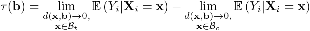
Under regularity conditions, which include smoothness of conditional expectations (see aforementioned references for details), the cutoff-specific treatment effects, τ(c) = E{Y_i (1) − Y_i (0)|X_i = c, C_i = c}, are identified by

$\tau (c) =\underset{x\downarrow c}{\lim }\mathbb{\text{E}}(Y_i|X_i =x, C_i =c)-\underset{x\uparrow c}{\lim }\text{E}(Y_i|X_i =x, C_i =c)$

The pooled RD estimate is obtained by recentering the running variable, $\tilde{X}$ _i = X_i −C_i , thus normalizing the cutoff at zero,

${\tau }_{\text{P}} = \underset{x\downarrow 0}{\lim }\mathbb{\text{E}}(Y_i|{\tilde{X}}_i =x)-\underset{x\uparrow 0}{\lim }\mathbb{\text{E}}(Y_i|{\tilde{X}}_i=x)$

1

where

$\begin{array}{l}{\tau }_{\text{P}}={\displaystyle \sum _{c\in \text{C}}\tau (c)\omega (c), }\\ \omega (c)=\frac{f_{X|C}(c|c)\mathbb{P}(C_{i }= c)}{{\displaystyle \sum _{c\in \text{C}}{f}_X{{ }_{|}}_C(c|c)\mathbb{P}(C_i =c)}}\end{array}$

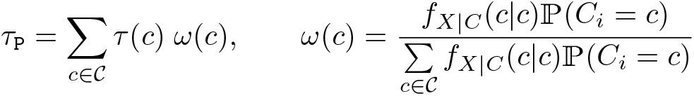
All of these parameters can be readily estimated using local polynomial methods (see Cattaneo, Idrobo, and Titiunik [2019] for a practical introduction), conditioning on cutoffs when appropriate. In other words, RD methods can be applied to each cutoff separately, in addition to pooling the data. Therefore, the rdmulti package implements bandwidth selection, estimation, and inference based on local polynomial methods using the rdrobust command, described in Calonico, Cattaneo, and Titiunik (2014a, 2015b) and Calonico et al. (2017). Specifically, the command rdmc allows for multicutoff RD designs.

For the pooled parameter τ _P , the weights are estimated using the fact that ω(c) =

$\omega \left(c\right) =\mathbb{P}(C_i =c|{\tilde{X}}_i=0)$ ; see Cattaneo et al. (2016) for further details. Then, given a band-width h > 0,

$\widehat{\omega }\left(c\right)=\frac{{\displaystyle {\sum }_i\mathbb{\text{1}}\left(C_i =c,-h\le {\tilde{X}}_i \le h\right)}}{{\displaystyle {\sum }_i\mathbb{\text{1}}\left(-h\le {\tilde{X}}_i \le h\right)}}$

When not specified by the user, the rdmc command uses the bandwidth selected by rdrobust when estimating the pooled effect to estimate the weights.

2.2 Cumulative multiple cutoffs

In an RD setting with cumulative cutoffs, individuals receive different treatments (or different dosages of a treatment) for different ranges of the running variable. In such a setting, individuals receive treatment 1 if X_i < c ₁, treatment 2 if c ₁ ≤ X_i < c ₂, and so on, until the last treatment value at X_i ≥ c_J . For example, Brollo et al. (2013) examine the effect of federal transfers on political corruption in Brazilian municipalities. The amount of the federal transfer that municipalities receive depends on the municipality’s population and changes discretely at specified cutoffs. For example, municipalities with population below 10,189 receive a certain amount, municipalities with population between 10,189 and 13,585 receive a larger amount, and so on.

Denote the values of these treatments as d_j , so that the treatment variable is now

D_i ∊ {d ₁ , d ₂ ,…d_J }. Under standard regularity conditions, we have

${\tau }_j =\mathbb{\text{E}}\{Y_i(d_j)-Y_i(d_j{{ }_{-}}_{\text{1}})|X_i =c_j\}= \underset{x\downarrow c_j}{\lim }\mathbb{\text{E}}(Y_i|X_i =x)-\underset{x\uparrow c_j}{\lim }\mathbb{\text{E}}(Y_i|X_i =x)$

Because, unlike the case with multiple noncumulative cutoffs, the population is not partitioned, each observation can be used to estimate two different (but contiguous on the score dimension) treatment effects. For example, units receiving treatment dosage d_j are used as “treated” (that is, above the cutoff c_j ) when estimating τ_j and as “controls” when estimating τ_{j +1} (that is, below the cutoff c_{j +1}). Thus, cutoff-specific estimators may not be independent, although the dependence disappears asymptotically as long as the bandwidths around each cutoff decrease with the sample size. On the other hand, bandwidths can be chosen to be nonoverlapping to ensure that observation ns are used only once.

Once the data have been assigned to each cutoff under analysis, local polynomial methods can also be applied cutoff by cutoff in the cumulative multiple cutoffs case. We illustrate this approach below; for further discussion see Cattaneo, Idrobo, and Titiunik (Forthcoming) and the references therein.

2.3 Multiple scores

In a multiscore RD design, treatment is assigned based on multiple running variables and some function determining a treatment “region” or “area”. We focus on the case with two running variables, X _i = (X _1i , X _2i ), which is by far the most common case in empirical work. This case occurs naturally when, for instance, a treatment is assigned based on scores in two different exams (such as language and mathematics). Matsudaira (2008) estimates the effect of a mandatory summer school program assigned to students who fail to score higher than a preset cutoff in both math and reading exams. Another common case of multiple running variables occurs when a treatment is assigned based on geographic location (for example, latitude and longitude). Keele and Titiunik (2015) discuss the effect of political campaign advertising on voter turnout and political attitudes by comparing voters in adjacent media markets, which result in different levels of exposure to advertising.

This type of assignment defines a continuum of treatment effects over the boundary of the treatment region, denoted by B . For instance, if treatment is assigned to students scoring below 50 in language and mathematics, the treatment boundary is B = {x ₁ ≤ 50, x ₂ = 50} ∪ {x ₁ = 50, x ₂ ≤ 50}. For each point b ∊ B , the treatment effect at that point is given by

$\tau \left(b\right) = \mathbb{\text{E}}\{Y_i\left(1\right)-Y_i\left(0\right)|X_i =b\}$

and under regularity conditions,

$\tau (b) = \underset{d(x,b)\to 0,x\in {\text{B}}_t}{\lim }\mathbb{\text{E}}(Y_i|X_i =x)-\underset{d(x,b)\to 0,x\in {\text{B}}_c}{\lim }\mathbb{\text{E}}(Y_i|X_i =x)$

where B _c and B _t denote the control and treatment areas, respectively, and d(·, ·) is a metric.

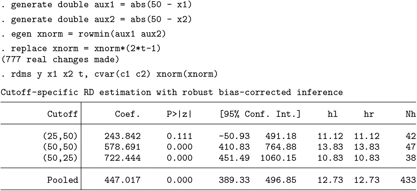
Because estimating a whole curve of treatment effects may not be feasible in practice, it is common to define a set of boundary points of interest at which to estimate the RD treatment effects. In the previous example, for instance, three points of interest on the boundary determining treatment assignment could be {(25, 50), (50, 50), (50, 25)}. On the other hand, the pooled RD estimand requires defining some measure of distance to the cutoff, such as the perpendicular (Euclidean) distance. This distance can be seen as the recentered running variable $\tilde{X}$ _i , which allows defining the pooled estimand as in (1).

3 The rdmc command

This section describes the syntax of the command rdmc, which estimates the pooled and cutoff-specific RD effects using rdrobust.

3.1 Syntax

depvar is the dependent variable. runvar is the running variable (also known as score or forcing variable).

3.2 Options

cvar( cutoff_var ) specifies the numeric variable cutoff_var, which indicates the cutoff faced by each unit in the sample. cvar() is required.

fuzzy( string ) indicates a fuzzy design. See help rdrobust for details.

derivvar( string ) specifies a variable of length equal to the number of different cutoffs that specifies the order of the derivative for rdrobust to calculate cutoff-specific estimates. See help rdrobust for details.

pooled_opt( string ) specifies the options to be passed to rdrobust to calculate pooled estimate. See help rdrobust for details.

verbose displays the output from rdrobust to calculate pooled estimand.

pvar( string ) specifies a variable of length equal to the number of different cutoffs that specifies the order of the polynomials for rdrobust to calculate cutoff-specific estimates. See help rdrobust for details.

qvar( string ) specifies a variable of length equal to the number of different cutoffs that specifies the order of the polynomials for bias estimation for rdrobust to calculate cutoff-specific estimates. See help rdrobust for details.

hvar( string ) specifies a variable of length equal to the number of different cutoffs that specifies the bandwidths for rdrobust to calculate cutoff-specific estimates. When hrightvar() is specified, hvar() indicates the bandwidth to the left of the cutoff. When hrightvar() is not specified, the same bandwidths are used at each side. See help rdrobust for details.

hrightvar( string ) specifies a variable of length equal to the number of different cutoffs that specifies the bandwidths to the right of the cutoff for rdrobust to calculate cutoff-specific estimates. When hrightvar() is not specified, the same bandwidths in hvar() are used at each side. See help rdrobust for details.

bvar( string ) specifies a variable of length equal to the number of different cutoffs that specifies the bandwidths for the bias for rdrobust to calculate cutoff-specific estimates. When brightvar() is specified, bvar() indicates the bandwidth to the left of the cutoff. When brightvar() is not specified, the same bandwidths are used at each side. See help rdrobust for details.

brightvar( string ) specifies a variable of length equal to the number of different cutoffs that specifies the bandwidths to the right of the cutoff for rdrobust to calculate cutoff-specific estimates. When brightvar() is not specified, the same bandwidths in bvar() are used at each side. See help rdrobust for details.

rhovar( string ) specifies a variable of length equal to the number of different cutoffs that specifies the value of rho for rdrobust to calculate cutoff-specific estimates. See help rdrobust for details.

covsvar( string ) specifies a variable of length equal to the number of different cutoffs that specifies the covariates for rdrobust to calculate cutoff-specific estimates. See help rdrobust for details.

covsdropvar( string ) specifies a variable of length equal to the number of different cutoffs that specifies whether collinear covariates should be dropped. See help rdro-bust for details.

kernelvar( string ) specifies a variable of length equal to the number of different cutoffs that specifies the kernels for rdrobust to calculate cutoff-specific estimates. See help rdrobust for details.

weightsvar( string ) specifies a variable of length equal to the number of different cutoffs that specifies the weights for rdrobust to calculate cutoff-specific estimates. See help rdrobust for details.

bwselectvar( string ) specifies a variable of length equal to the number of different cutoffs that specifies the bandwidth selection method for rdrobust to calculate cutoff-specific estimates. See help rdrobust for details.

scaleparvar( string ) specifies a variable of length equal to the number of different cutoffs that specifies the value of scaleparvar() for rdrobust to calculate cutoff- specific estimates. See help rdrobust for details.

scaleregulvar( string ) specifies a variable of length equal to the number of different cutoffs that specifies the value of scaleregulvar() for rdrobust to calculate cutoff- specific estimates. See help rdrobust for details.

masspointsvar( string ) specifies a variable of length equal to the number of different cutoffs that specifies how to handle repeated values in the running variable. See help rdrobust for details.

bwcheckvar( string ) specifies a variable of length equal to the number of different cutoffs that specifies the value of bwcheckvar(). See help rdrobust for details.

bwrestrictvar( string ) specifies a variable of length equal to the number of different cutoffs that specifies whether computed bandwidths are restricted to the range of runvar. See help rdrobust for details.

stdvarsvar( string ) specifies a variable of length equal to the number of different cutoffs that specifies whether depvar and runvar are standardized. See help rdrobust for details.

vcevar( string ) specifies a variable of length equal to the number of different cutoffs that specifies the variance–covariance matrix estimation method for rdrobust to calculate cutoff-specific estimates. See help rdrobust for details.

level( # ) specifies the confidence levels for confidence intervals. See help rdrobust for details.

plot plots the pooled and cutoff-specific estimates and the weights given by the pooled estimate to each cutoff-specific estimate.

graph_opt( string ) specifies options to be passed to the graph when plot is specified.

4 The rdmcplot command

This section describes the syntax of the command rdmcplot, which plots the regression functions for each of the groups facing each cutoff using rdplot.

4.1 Syntax

depvar is the dependent variable. runvar is the running variable (also known as score or forcing variable).

4.2 Options

cvar( cutoff_var ) specifies the numeric variable cutoff_var, which indicates the cutoff faced by each unit in the sample. cvar() is required.

nbinsvar( string ) specifies a variable of length equal to the number of different cutoffs that specifies the number of bins for rdplot. When nbinsrightvar() is specified, nbinsvar() indicates the number of bins to the left of the cutoff. When nbinsrightvar() is not specified, the same number of bins is used at each side. See help rdplot for details.

nbinsrightvar( string ) specifies a variable of length equal to the number of different cutoffs that specifies the number of bins to the right of the cutoff for rdplot. When nbinsrightvar() is not specified, the same number of bins in nbinsvar() is used at each side. See help rdplot for details.

binselectvar( string ) specifies a variable of length equal to the number of different cutoffs that specifies the bin selection method for rdplot. See help rdplot for details.

scalevar( string ) specifies a variable of length equal to the number of different cutoffs that specifies the scale for rdplot. When scalerightvar() is specified, scalevar() indicates the scale to the left of the cutoff. When scalerightvar() is not specified, the same scale is used at each side. See help rdplot for details.

scalerightvar( string ) specifies a variable of length equal to the number of different cutoffs that specifies the scale to the right of the cutoff for rdplot. When scalerightvar() is not specified, the scale in scalevar() is used at each side. See help rdplot for details.

supportvar( string ) specifies a variable of length equal to the number of different cutoffs that specifies the support for rdplot. When the option supportrightvar() is specified, supportvar() indicates the support to the left of the cutoff. When supportrightvar() is not specified, the same support is used at each side. See help rdplot for details.

supportrightvar( string ) specifies a variable of length equal to the number of different cutoffs that specifies the support to the right of the cutoff for rdplot. When supportrightvar() is not specified, the support in supportvar() is used at each side. See help rdplot for details.

pvar( string ) specifies a variable of length equal to the number of different cutoffs that specifies the order of the polynomials for rdplot. See help rdplot for details.

hvar( string ) specifies a variable of length equal to the number of different cutoffs that specifies the bandwidths for rdplot. When hrightvar() is specified, hvar() indicates the bandwidth to the left of the cutoff. When hrightvar() is not specified, the same bandwidth is used at each side. See help rdplot for details.

hrightvar( string ) specifies a variable of length equal to the number of different cutoffs that specifies the bandwidth to the right of the cutoff for rdplot. When hrightvar() is not specified, the bandwidth in hvar() is used at each side. See help rdplot for details.

kernelvar( string ) specifies a variable of length equal to the number of different cutoffs that specifies the kernels for rdplot. See help rdplot for details.

weightsvar( string ) specifies a variable of length equal to the number of different cutoffs that specifies the weights for rdplot. See help rdplot for details.

covsvar( string ) specifies a variable of length equal to the number of different cutoffs that specifies the covariates for rdplot. See help rdplot for details.

covsevalvar( string ) specifies a variable of length equal to the number of different cutoffs that specifies the evaluation points for additional covariates. See help rdplot for details.

covsdropvar( string ) specifies a variable of length equal to the number of different cutoffs that specifies whether collinear covariates should be dropped. See help rdplot for details.

binsoptvar( string ) specifies a variable of length equal to the number of different cutoffs that specifies options for the bins plots.

lineoptvar( string ) specifies a variable of length equal to the number of different cutoffs that specifies options for the polynomial plots.

xlineoptvar( string ) specifies a variable of length equal to the number of different cutoffs that specifies options for the vertical lines indicating the cutoffs.

ci( cilevel ) adds confidence intervals of level cilevel to the plot.

nobins omits the bins plot.

nopoly omits the polynomial curve plot.

noxline omits the vertical lines indicating the cutoffs.

nodraw omits the plot.

genvars generates variables to replicate plots by hand. Variable labels indicate the corresponding cutoff.

rdmcplot_hat_y_ c is the predicted value of the outcome variable given by the global polynomial estimator in cutoff number c.

rdmcplot_mean_x_ c is the sample mean of the running variable within the corresponding bin for each observation in cutoff number c.

rdmcplot_mean_y_ c is the sample mean of the outcome variable within the corresponding bin for each observation in cutoff number c.

rdmcplot_ci_l_ c is the lower end value of the confidence interval for the sample mean of the outcome variable within the corresponding bin for each observation in cutoff number c.

rdmcplot_ci_r_ c is the upper end value of the confidence interval for the sample mean of the outcome variable within the corresponding bin for each observation in cutoff number c.

5 The rdms command

This section describes the syntax of the command rdms, which analyzes RD designs with cumulative cutoffs or two running variables.

5.1 Syntax

depvar is the dependent variable. runvar1 is the running variable (also known as score or forcing variable) in a cumulative cutoffs setting. runvar2, if specified, is the second running variable (also known as score or forcing variable) in a two-score setting. treatvar, if specified, is the treatment indicator in a two-score setting.

5.2 Options

cvar( cutoff_var1 [cutoff_var2] ) specifies the numeric variable cutoff_var1, which indicates the cutoff faced by each unit in the sample in a cumulative cutoff setting, or the two running variables cutoff_var1 and cutoff_var2 in a two-score RD design. cvar() is required.

range( range1 [range2] ) specifies the range of the running variable to be used for estimation around each cutoff. Specifying only one variable implies using the same range at each side of the cutoff.

xnorm( string ) specifies the normalized running variable to estimate pooled effect.

fuzzy( string ) indicates a fuzzy design. See help rdrobust for details.

derivvar( string ) specifies a variable of length equal to the number of different cutoffs that specifies the order of the derivative for rdrobust to calculate cutoff-specific estimates. See help rdrobust for details.

pooled_opt( string ) specifies the options to be passed to rdrobust to calculate pooled estimate. See help rdrobust for details.

pvar( string ) specifies a variable of length equal to the number of different cutoffs that specifies the order of the polynomials for rdrobust to calculate cutoff-specific estimates. See help rdrobust for details.

qvar( string ) specifies a variable of length equal to the number of different cutoffs that specifies the order of the polynomials for bias estimation for rdrobust to calculate cutoff-specific estimates. See help rdrobust for details.

hvar( string ) specifies a variable of length equal to the number of different cutoffs that specifies the bandwidths for rdrobust to calculate cutoff-specific estimates. When hrightvar() is specified, hvar() indicates the bandwidth to the left of the cutoff. When hrightvar() is not specified, the same bandwidths are used at each side. See help rdrobust for details.

hrightvar( string ) specifies a variable of length equal to the number of different cutoffs that specifies the bandwidths to the right of the cutoff for rdrobust to calculate cutoff-specific estimates. When hrightvar() is not specified, the same bandwidths in hvar() are used at each side. See help rdrobust for details.

bvar( string ) specifies a variable of length equal to the number of different cutoffs that specifies the bandwidths for the bias for rdrobust to calculate cutoff-specific estimates. When brightvar() is specified, bvar() indicates the bandwidth to the left of the cutoff. When brightvar() is not specified, the same bandwidths are used at each side. See help rdrobust for details.

brightvar( string ) specifies a variable of length equal to the number of different cutoffs that specifies the bandwidths to the right of the cutoff for rdrobust to calculate cutoff-specific estimates. When brightvar() is not specified, the same bandwidths in bvar() are used at each side. See help rdrobust for details.

rhovar( string ) specifies a variable of length equal to the number of different cutoffs that specifies the value of rho for rdrobust to calculate cutoff-specific estimates. See help rdrobust for details.

covsvar( string ) specifies a variable of length equal to the number of different cutoffs that specifies the covariates for rdrobust to calculate cutoff-specific estimates. See help rdrobust for details.

covsdropvar( string ) specifies a variable of length equal to the number of different cutoffs that specifies whether collinear covariates should be dropped. See help rdro-bust for details.

kernelvar( string ) specifies a variable of length equal to the number of different cutoffs that specifies the kernels for rdrobust to calculate cutoff-specific estimates. See help rdrobust for details.

weightsvar( string ) specifies a variable of length equal to the number of different cutoffs that specifies the weights for rdrobust to calculate cutoff-specific estimates. See help rdrobust for details.

bwselectvar( string ) specifies a variable of length equal to the number of different cutoffs that specifies the bandwidth selection method for rdrobust to calculate cutoff-specific estimates. See help rdrobust for details.

scaleparvar( string ) specifies a variable of length equal to the number of different cutoffs that specifies the value of scaleparvar() for rdrobust to calculate cutoff- specific estimates. See help rdrobust for details.

scaleregulvar( string ) specifies a variable of length equal to the number of different cutoffs that specifies the value of scaleregulvar() for rdrobust to calculate cutoff- specific estimates. See help rdrobust for details.

masspointsvar( string ) specifies a variable of length equal to the number of different cutoffs that specifies how to handle repeated values in the running variable. See help rdrobust for details.

bwcheckvar( string ) specifies a variable of length equal to the number of different cutoffs that specifies the value of bwcheckvar(). See help rdrobust for details.

bwrestrictvar( string ) specifies a variable of length equal to the number of different cutoffs that specifies whether computed bandwidths are restricted to the range of runvar. See help rdrobust for details.

stdvarsvar( string ) specifies a variable of length equal to the number of different cutoffs that specifies whether depvar and runvar are standardized. See help rdrobust for details.

vcevar( string ) specifies a variable of length equal to the number of different cutoffs that specifies the variance–covariance matrix estimation method for rdrobust to calculate cutoff-specific estimates. See help rdrobust for details.

level( # ) specifies the confidence levels for confidence intervals. See help rdrobust for details.

plot plots the pooled and cutoff-specific estimates and the weights given by the pooled estimate to each cutoff-specific estimate.

graph_opt( string ) specifies options to be passed to the graph when plot is specified.

6 Illustration of methods

6.1 Noncumulative multiple cutoffs

We begin by illustrating rdmc using a simulated dataset, simdata_multic.dta. In this dataset, y is the outcome variable, x is the running variable, c is a variable indicating the cutoff that each unit in the sample faces, and t is a treatment indicator, corresponding in this case to units with x ≥ c. As shown below, there are two different cutoffs, 33 and 66, each with the same size.

The basic syntax for rdmc is the following:

The output shows the cutoff-specific estimate at each cutoff, together with the corresponding robust bias-corrected p-value, 95% robust confidence interval and sample size at each cutoff, and two “global” estimates. The first one is a weighted average of the cutoff-specific estimates using the estimated weights described in section 2. These estimated weights are shown in the last column. The second one is the pooled estimate obtained by normalizing the running variable. While these two estimators converge to the same population parameter, they can differ in finite samples as seen above. In this example, the effect is statistically significant at both cutoffs.

All the results in the above display are calculated using rdrobust. The user can specify options for rdrobust to calculate the pooled estimates using pooled_opt(). For instance, the syntax below specifies a bandwidth of 20 and a local quadratic polynomial for the pooled estimand. By default, rdmc omits the output from rdrobust when estimating the effects. The output from the pooled effect estimation can be displayed using the option verbose, which we use below to show how the options are passed to rdrobust.

The user can also modify the options for estimation in each specific cutoff. The following syntax shows how to manually change options for the cutoff-specific estimates by setting a bandwidth of 11 in the first cutoff and 10 in the second one.

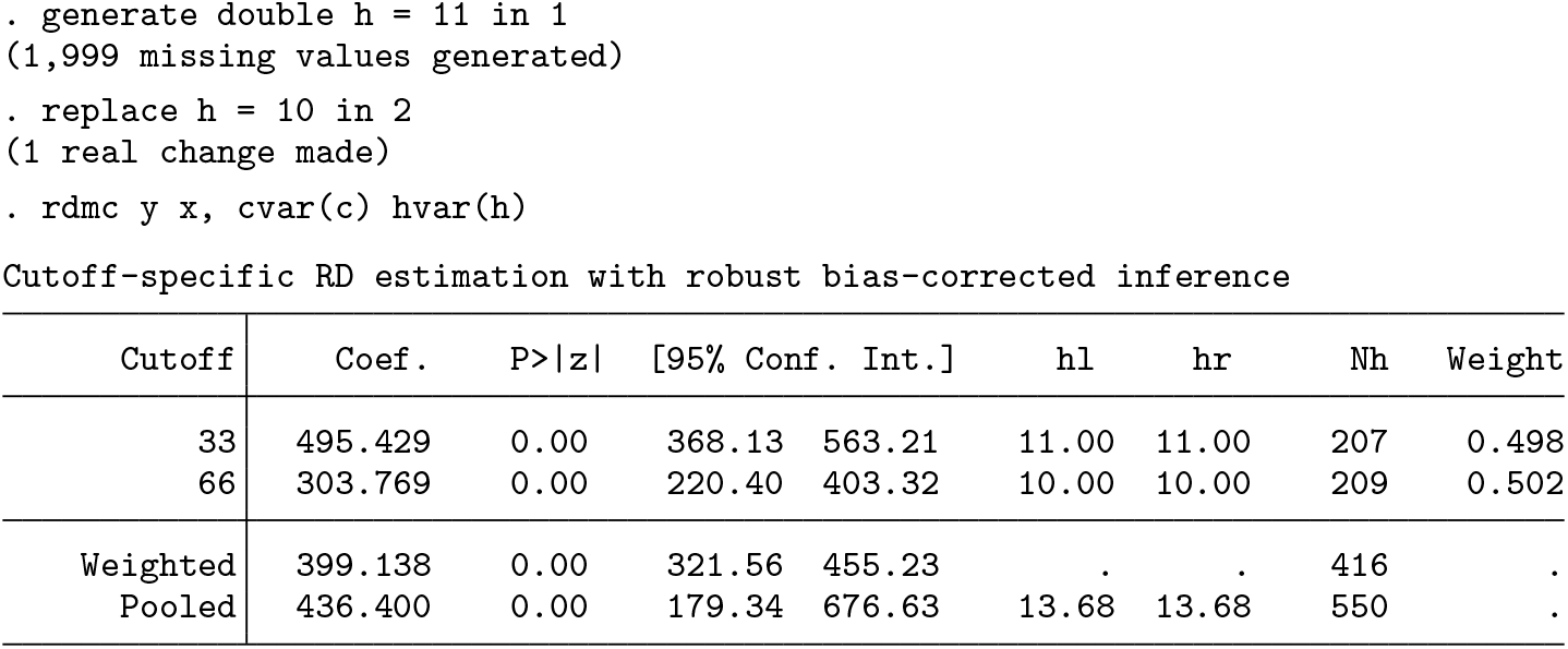
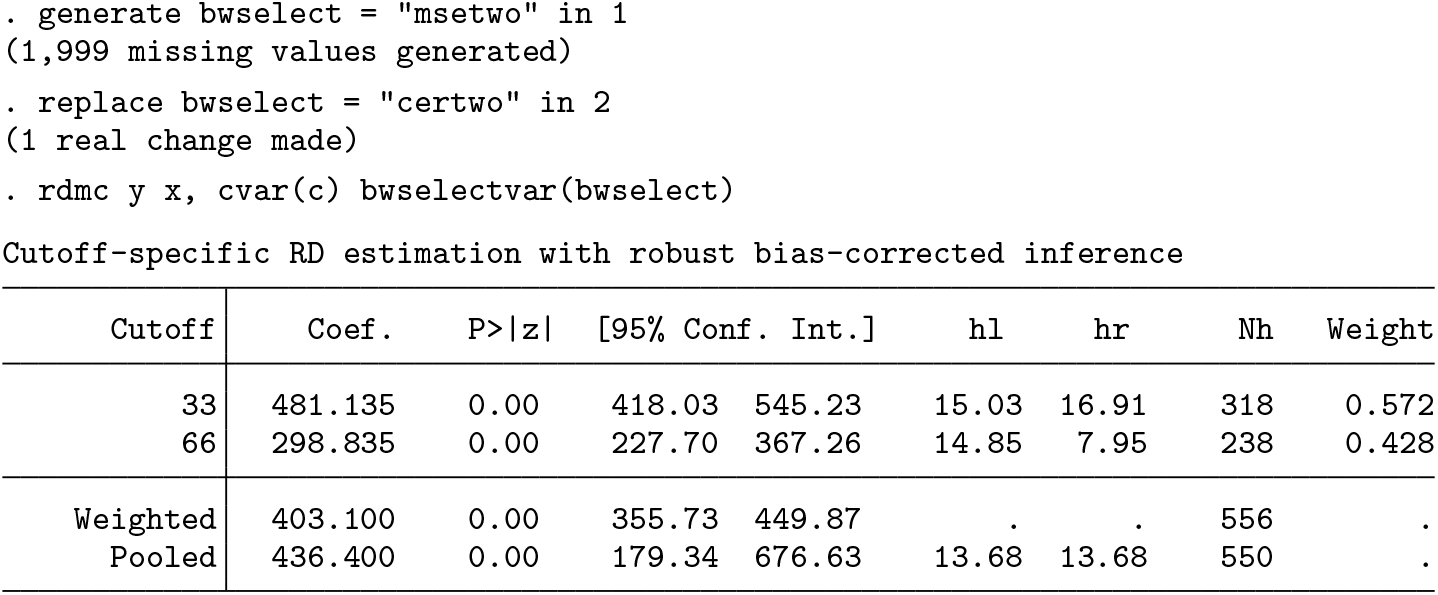
All the cutoff-specific options are passed in a similar fashion, defining a new variable of length equal to the number of cutoffs that indicates the options for each cutoff in its values. For instance, the following syntax indicates different bandwidth selection methods at each cutoff:

The rdmc command saves the bias-corrected estimates and variances in the matrices e(b) and e(V), which allows for postestimation testing using lincom or test. For instance, to test whether the effects at the two cutoffs are the same, type

The rdmcplot command jointly plots the estimated regression functions at each cutoff. The output from rdmcplot is shown in figure 1. The basic syntax is the following:

Figure 1.

Multiple RD plot

The rdmcplot includes all the options available for rdplot. For example, the plot can be restricted to a bandwidth using the option hvar() and to use a polynomial of a specified order using the option pvar(), as shown below. This option allows the user to plot the linear fit and estimated treatment effects at each cutoff.

The resulting plot is shown in figure 2.

Figure 2.

Multiple RD plot

The option genvars generates the variables required to replicate the plots by hand. This allows the user to customize the plot. The following code illustrates how to use this option to replicate figure 2.

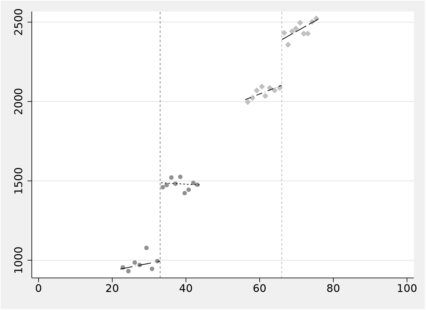
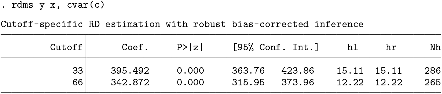
6.2 Cumulative multiple cutoffs

We now illustrate the use of rdms for cumulative cutoffs using a simulated dataset, simdata_cumul.dta. In this dataset, the running variable ranges from 0 to 100, and units with a running variable below 33 receive a certain treatment level d ₁, whereas units with a running variable above 66 receive another treatment level d ₂. In this setting, the cutoffs are indicated as a variable in the dataset, where each row indicates a cutoff.

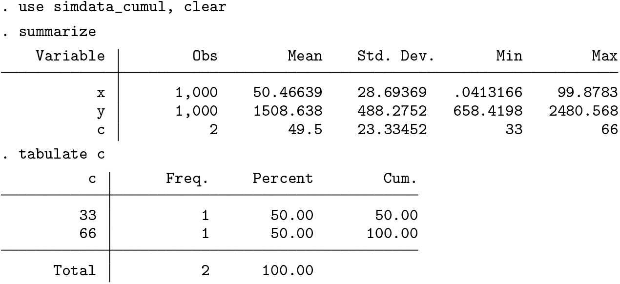
The syntax for cumulative cutoffs is similar to rdmc. The user specifies the outcome variable, the running variable, and the cutoffs as follows:

Options like the bandwidth, polynomial order, and kernel for each cutoff-specific effect can be specified by creating variables as shown below.

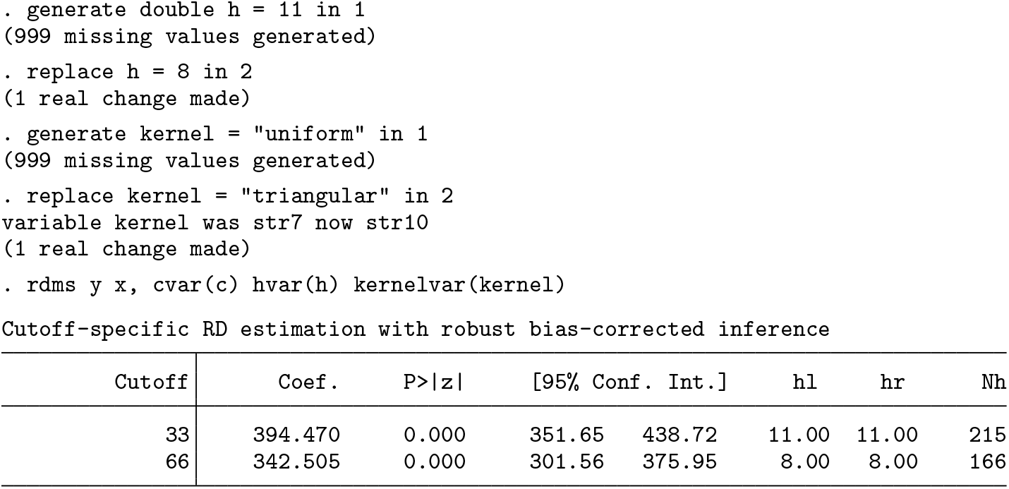
Without further information, the rdms command could be using any observation above the cutoff 33 to estimate the effect of the first treatment level d ₁. This implies that some observations in the range [66, 100] are used. But these observations receive the second treatment level, d ₂. This feature can result in inconsistent estimators for τ ₁. To avoid this problem, the user can specify the range of observations to be used around each cutoff. In this case, we can restrict the range at the first cutoff (33) to go from 0 to 65.5 to ensure that no observations above 66 are used and the range at the second cutoff (66) to go from 33.5 to 100. This can be done as follows.

The pooled estimate can be obtained using rdmc. For this, we need to assign each unit in the sample a value for the cutoff. One possibility is to assign each unit to the closest cutoff. For this, we generate a variable named cutoff that equals 33 for units with score below 49.5 (the middle point between 33 and 66) and equals 66 for units above 49.5.

Finally, we can use the variable cutoff to plot the regression functions using the command rdmcplot, shown in figure 3.

Figure 3.

Cumulative cutoffs

6.3 Multiple scores

We now illustrate the use of rdms to analyze RD designs with two running variables using a simulated dataset, simdata_multis.dta. In this dataset, there are two running variables, x1 and x2, ranging between 0 and 100, and units receive the treatment when x1 ≤ 50 and x2 ≤ 50. We look at three cutoffs on the boundary: (25, 50), (50, 50), and (50, 25).

The following code provides a simple visualization of this setting, shown in figure 4:

Figure 4.

Bivariate score

The basic syntax is the following:

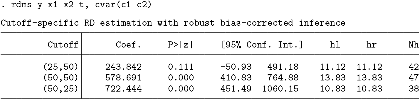
Information to estimate each cutoff-specific estimate can be provided as illustrated before. For instance, to specify cutoff-specific bandwidths, type

Finally, the xnorm() option allows the user to specify the normalized running variable to calculate a pooled estimate. In this case, we define the normalized running variable as the closest perpendicular distance to the boundary defined by the treatment assignment, with positive values indicating treated units and negative values indicating control units.

7 Conclusion

We introduced the package rdmulti to analyze RD designs with multiple cutoffs or scores. A companion R function with the same syntax and capabilities was also provided.

Supplemental Material

Supplemental Material, st0620 - Analysis of regression-discontinuity designs with multiple cutoffs or multiple scores

Supplemental Material, st0620 for Analysis of regression-discontinuity designs with multiple cutoffs or multiple scores by Matias D. Cattaneo, Rocío Titiunik and Gonzalo Vazquez-Bare in The Stata Journal