Sage Journals: Discover world-class research

Abstract

In this article, we introduce two commands, rdpow and rdsampsi, that conduct power calculations and survey sample selection when using local polynomial estimation and inference methods in regression-discontinuity designs. rdpow conducts power calculations using modern robust bias-corrected local polynomial inference procedures and allows for new hypothetical sample sizes and bandwidth selections, among other features. rdsampsi uses power calculations to compute the minimum sample size required to achieve a desired level of power, given estimated or user-supplied bandwidths, biases, and variances. Together, these commands are useful when devising new experiments or surveys in regression-discontinuity designs, which will later be analyzed using modern local polynomial techniques for estimation, inference, and falsification. Because our commands use the communitycontributed (and R) package rdrobust for the underlying bandwidths, biases, and variances estimation, all the options currently available in rdrobust can also be used for power calculations and sample-size selection, including preintervention covariate adjustment, clustered sampling, and many bandwidth selectors. Finally, we also provide companion R functions with the same syntax and capabilities.

Keywords

st0554 rdpow rdsampsi regression-discontinuity designs power calculations local polynomial methods

1 Introduction

Power calculations are used when designing experiments and field work in various disciplines in social, behavioral, and medical sciences. Recently, many empirical researchers have designed and implemented surveys using regression-discontinuity (RD) designs. See Imbens and Lemieux (2008); Lee and Lemieux (2010); Calonico, Cattaneo, and Titiunik (2015a); Cattaneo and Escanciano (2017); Cattaneo, Titiunik, and Vazquez-Bare (2017); Cattaneo, Idrobo, and Titiunik (Forthcoming a,b); and references therein for introductions to RD designs. In this article, we introduce two commands (and companion R functions) specifically developed to conduct power calculations and survey sample selection when using RD local polynomial estimation and inference methods.

There are two main approaches to interpret and analyze RD designs in modern applied work. The first approach is based on continuity or smoothness assumptions and typically uses local polynomial methods (for example, Calonico, Cattaneo, and Titiunik [2014b]; Calonico, Cattaneo, and Farrell [2018a,b,c]; Calonico et al. [Forthcoming]; and references therein). The second approach is based on a local (to the RD cutoff) independence assumption and hence uses ideas and methods from the classical literature on the analysis of experiments (Cattaneo, Frandsen, and Titiunik [2015]; Cattaneo, Titiunik, and Vazquez-Bare [2017]; Sekhon and Titiunik [2017]; and references therein). Both methods can be used for estimation, inference, and falsification in empirical work using RD designs.

In this article, we focus on local polynomial methods and introduce the commands rdpow and rdsampsi, which allow for power calculations and sample selection based on large-sample approximations under continuity or smoothness assumptions. rdpow conducts power calculations using modern robust bias-corrected local polynomial inference procedures and allows for new hypothetical sample sizes and bandwidth selections, among other features. The companion command rdsampsi uses power calculations to compute the minimum sample size required to achieve a desired level of power. Both commands also offer graphical presentation of the main results. Together, these commands are particularly useful when devising new experiments or surveys in RD design settings, assuming they will later be analyzed using modern local polynomial techniques for estimation, inference, and falsification.

The underlying main calculations (bandwidth selection, bias estimation, and variance estimation) in both commands rely on the package rdrobust (available in both Stata and R; see Calonico, Cattaneo, and Titiunik [2014a,b] and Calonico et al. [2017] for more details). This implies that all the options and features available in rdrobust can be used when using our power calculation and sample selection implementations. In particular, our commands allow for clustered sampling, preintervention covariate adjustment, and different bandwidth selectors, among many other possibilities and features.

Our two commands complement the recently introduced Stata and R commands for RD designs. See Calonico, Cattaneo, and Titiunik (2014a, 2015b) and Calonico et al. (2017) for an introduction to the commands rdrobust, rdbwselect, and rdplot for graphical presentation, estimation, and inference in RD designs using nonparametric local polynomial techniques. See Cattaneo, Titiunik, and Vazquez-Bare (2016) for an introduction to the commands rdrandinf, rdwinselect, rdsensitivity, and rdrbounds for implementing randomization-based inference methods for RD designs under a local randomization assumption. See Cattaneo, Jansson, and Ma (2018b) for an introduction to rddensity and rdbwdensity for manipulation testing using the methods developed in Cattaneo, Jansson, and Ma (2018a).

The rest of the article is organized as follows: Section 2 briefly reviews the main conceptual and methodological issues underlying power calculations for RD designs when using local polynomial inference techniques. Sections 3 and 4 provide details on the syntax of the commands rdpow and rdsampsi, respectively. Section 5 gives a detailed empirical illustration, and section 6 concludes.

The latest version of this software and related software for RD designs can be found at https://sites.google.com/site/rdpackages/.

2 Overview of methods

We briefly describe the main formulas and methods used in the commands rdpow and rdsampsi to conduct power calculations and sample selection in RD designs when using local polynomial methods for estimation, inference, and falsification testing. As clarified below, the main formulas and methods require estimating several unknown quantities such as bandwidths, biases, and variances, which are all estimated using the package rdrobust (whenever not provided directly by the user). We do not discuss these estimators here but rather refer the reader to Calonico, Cattaneo, and Titiunik (2014a, 2015b), Calonico et al. (2017), and the references therein for further details.

Analyzing the statistical power of widely used RD inference procedures is important for at least two distinct reasons. We briefly mention both now, but we will further discuss them below in our methodology summary (this section) and in our numerical illustration (section 5).

Ex-post (or observational) RD analysis. The researcher already has the final data for analysis, and the goal is to assess the statistical power underlying the testing procedures implemented in rdrobust. Specifically, rdpow will estimate the statistical power of the robust bias-corrected inference methods implemented using rdrobust for a given hypothesized RD treatment effect (denoted τ _A below). In this case, the sample size is fixed, and the goal is to understand the statistical power that different inference procedures have. For example, the researcher can compare the statistical power between using local linear and local quadratic methods.

Ex-ante (or experimental) RD design. The researcher is designing a new survey for an RD design, and the final data are not available yet. In some circumstances, for instance, the RD design might be a preferable alternative to a classical random assignment design, especially when such design is unfeasible for some reason (ethical or otherwise). For example, the RD design allows for a normal program operation—as opposed to purely randomized designs—because treatment assignments for the study population are determined by rules developed by program staff or policymakers rather than randomly assigned. In this sense, the treatment can be targeted to those who normally receive them (for evaluations of existing interventions) or to those who are likely to benefit most from them (for evaluations of new interventions). In this case, rdsampsi implicitly uses power calculations. The main goal of rdsampsi is to compute the minimal sample sizes needed to achieve a desired level of power when the final dataset will be analyzed using the testing procedures implemented in rdrobust. Typically, larger sample sizes are required in RD designs to construct inference procedures with the same level of statistical power as in classical randomized experiments.

The methods developed and implemented in this article are useful for both ex-post analysis and ex-ante design. In the remainder of this section, we first review classical design of experiments in the context of randomized control trials and then present the corresponding methodology for RD designs.

2.1 Review: Experimental designs

We first review standard approaches for power calculations and sample selection in simple experiments or randomized control trials. Suppose {(Y_i, T_i ) : 1 ≤ i ≤ n} is a random sample from a large population, with T_i denoting treatment status and Y_i = (1−T_i )Y_i (0)+T_iY_i (1), with Y_i (0) and Y_i (1) denoting the underlying potential outcomes without and with treatment, respectively. Here, by assumption, T_i is statistically independent of [Y_i (0), Y_i (1)].

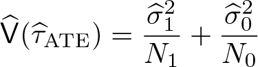
We assume the population parameter of interest is the average treatment effect $(ATE) τ_{ATE} = E [Y_{i} (1) - Y_{i} (0)]$ . To fix ideas, we consider the standard difference-in-means point estimator and corresponding t test statistic. The point estimator compares the difference in means between treated and control units,

{\hat{τ}}_{ATE} = {\bar{Y}}_{1} - {\bar{Y}}_{0}, Y_{1} = \frac{1}{N_{1}} \sum_{i = 1}^{n} T_{i} Y_{i}, {\bar{Y}}_{0} = \frac{1}{N_{0}} \sum_{i = 1}^{n} i = 1 (1 - T_{i}) Y_{i}

where N ₀ and N ₁ are the sample sizes of the control and treatment groups, respectively. If we employ a central limit theorem under appropriate regularity conditions, and if τ is the true ATE (for example, τ = τ _ATE under the true model), then

t_{ATE} (τ) = \frac{{\hat{τ}}_{ATE} - τ}{\sqrt{V ({\hat{τ}}_{ATE})}} \to_{d} N (0, 1), V ({\hat{τ}}_{ATE}) = \frac{σ_{1}^{2}}{N_{1}} + \frac{σ_{0}^{2}}{N_{0}}

where $σ_{0}^{2} = V [Y_{i} (0)]$ and $σ_{1}^{2} = V [Y_{i} (1)]$ are the population variances of the control and treatment groups, respectively. In practice, the two unknown variances are estimated, for instance, by

{\hat{σ}}_{0}^{2} = \frac{1}{N_{0} - 1} \sum_{i = 1}^{n} (1 - T_{i}) {(Y_{i} - Y_{0})}^{2} and {\hat{σ}}_{1}^{2} = \frac{1}{N_{1} - 1} \sum_{i = 1}^{n} T_{i} {(Y_{i} - Y_{1}}^{2})

respectively. Consider the two-sided hypothesis testing problem:

H_{0} : τ = 0 versus H_{A} : τ = τ_{A} \neq 0

Then, the associated (asymptotic) two-sided α-level power function based on the t test statistic and large-sample distribution theory given above is

β_{ATE} (τ) = 1 - Φ (\frac{τ}{V ({\hat{τ}}_{ATE})} + z_{1 - α / 2}) + Φ (\frac{τ}{V ({\hat{τ}}_{ATE})} - z_{1 - α / 2})

where Φ(·) denotes the cumulative distribution function of the standard normal distribution and z_a denotes its a quantile; that is, z_a = Φ⁻¹(a). In practice, $V ({\hat{τ}}_{A T E})$ is replaced by the consistent estimator

\hat{V} ({\hat{τ}}_{ATE}) = \frac{{\hat{σ}}_{1}^{2}}{N_{1}} + \frac{{\hat{σ}}_{0}^{2}}{N_{0}}

Given the parameter of interest (τ _ATE) and test statistic [t _ATE(τ)], one can use the large-sample Gaussian approximation to determine i) the total sample size n = N ₀ + N ₁ needed to achieve a predetermined level of power against a given alternative hypothesis and ii) the optimal assignment of relative sample sizes N ₀ and N ₁. We briefly discuss these choices next because the same logic will be used further below for RD designs. For simplicity and without loss of generality, we set τ _ATE = 0.

First, we determine the optimal relative sample size between control and treatment groups by minimizing the asymptotic variance of the estimator, given an overall choice of sample size n = N ₀ + N ₁. To be specific, set ϱ = N ₁ /n, and observe that minimizing $V ({\hat{τ}}_{A T E})$ with respect to ϱ gives the optimal choice:

ϱ = \frac{σ_{1}}{σ_{0} + σ_{1}}

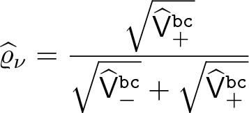
For example, if σ ₀ = σ ₁, then ϱ = 1/2; thus, equal sample sizes for control and treatment units are chosen. More generally, this approach leads to a relatively larger sample size for the group with a relatively larger variability in the outcome variable. This optimal choice of sample-size assignment between control and treatment groups is easily estimable in practice: $\hat{σ} = {\hat{σ}}_{1} / ({\hat{σ}}_{0} + {\hat{σ}}_{1})$

Second, given the choice of ϱ, we determine the total sample size

n = N_{0} + N_{1}, N_{0} = (1 - ϱ) n, N_{1} = ϱ n

using the (asymptotic) power function. Specifically, given a choice of alternative τ _A 6= 0 (usually determined as a fraction of σ ₀) and the desired power β ∈ [0, 1] (usually set at β = 80%), the overall sample size n is chosen as the unique integer value n solving the equation β = β _ATE(τ _A); that is,

n solves : β = 1 - Φ (\frac{τ_{A}}{\sqrt{\frac{σ_{1}^{2}}{ϱ n} + \frac{σ_{0}^{2}}{(1 - ϱ) n}}} + z_{1 - α / 2}) + Φ (\frac{τ_{A}}{\sqrt{\frac{σ_{1}^{2}}{ϱ n} + \frac{σ_{0}^{2}}{(1 - ϱ) n}}} - z_{1 - α / 2})

where the only unknown is n after ϱ, $σ_{0}^{2}$ , and $σ_{1}^{2}$ are replaced by their corresponding estimators $\hat{σ}$ , ${\hat{σ}}_{0}^{2}$ , and ${\hat{σ}}_{1}^{2}$ , as commonly done in practice.

The approach above is used in empirical work to determine the total sample size, n, and the relative proportion of sample sizes of control and treatment units, ϱ. In the following sections, we build on these ideas and apply them to the context of RD designs using local polynomial methods.

2.2 Regression discontinuity designs

For the remainder of this article, we study power calculation and sample selection in RD designs. We assume that {(Y_i, T_i, X_i ) : 1 ≤ i ≤ n} is a random sample from a large population, where for each unit i in the sample, Y_i = (1 − T_i )Y_i (0) + T_iY_i (1) is the outcome variable, with Y_i (0) and Y_i (1) denoting the underlying potential outcomes without and with treatment; T_i = $1$ (X_i < c)T_i (0) + $1$ (X_i ≥ c)T_i (1) is the treatment status, with T_i (0) and T_i (1) denoting the underlying potential treatment status; X_i denotes the so-called running variable, score, or index; and c denotes the RD cutoff. In RD designs, treatment assignment for each unit is determined based on whether the score X_i exceeds the known cutoff c. We cover all possible RD cases simultaneously; therefore, we do not assume perfect compliance. That is, we do not force T_i = $1$ (X_i ≥ c) as in sharp RD designs.

Our presentation is sufficiently high level enough that we avoid unnecessary repetition and overwhelming notation required to discuss each RD setting in detail, so we refer the reader to Calonico et al. (2017) and the references therein for specific details. To be more concrete, we denote a generic RD parameter of interest by τ _ν , where ν = 0, 1,…, p traces out the specific cases: i) ν = 0 corresponds to sharp RD cases (for example, the average sharp RD treatment effect at the cutoff τ ₀ = $E$ [Y_i (1) − Y_i (0)|X_i = c], or the fuzzy RD estimand ς ₀ = $E$ [Y_i (1)−Y_i (0)|X_i = c, compliers]); and ii) ν = 1 corresponds to kink RD cases (for example, τ ₁ = ∂ $E$ [Y_i (1)−Y_i (0)|X_i = c]/∂c corresponds to the average sharp kink RD treatment effect at the cutoff, and ς ₁ is the corresponding fuzzy–kink RD estimand).

To describe how to do power calculations and sample selection in RD designs, and continuing with our high level of generality, we let τb _ν denote a generic (pth order) local polynomial estimator constructed with bandwidths h ₋ (for left estimation) and h ₊ (for right estimation) of the corresponding RD treatment effect τ _ν . Then, under regularity conditions and bandwidth sequence restrictions, the following distributional approximation holds whenever τ is the population RD treatment effect (for example, τ = τ _ν under the true model):

\frac{{\hat{τ}}_{ν} - τ - B}{\sqrt{V}} \to_{d} N (0, 1)

with

B = h_{+}^{1 + p - ν} B_{+} - h_{-}^{1 + p - ν} B_{-}, V = \frac{1}{n h_{+}^{1 + 2 ν}} V_{+} + \frac{1}{n h_{-}^{1 + 2 ν}} V_{-}

B₋ and B₊ denote the left and right (to the RD cutoff) misspecification biases, and V₋ and V₊ denote the left and right (to the RD cutoff) asymptotic variance of the RD estimator. Depending on the estimand and estimator under consideration, the exact form of these quantities is different. Nevertheless, the generic result above applies to all main RD cases at this level of generality, including cases where the estimand of interest is the fuzzy, kink, or fuzzy–kink RD parameter; cases where preintervention covariate adjustment is considered; and cases where clustered sampling is present. For more details, see Calonico, Cattaneo, and Titiunik (2014b) as well as Calonico et al. (Forthcoming) and references therein.

We use the generic large-sample Gaussian distributional approximation in (1) to construct asymptotic power functions and to select sample sizes for survey design based on them. Without loss of generality, we assume τ _ν = 0 in the rest of this article.

Power calculations with misspecification bias

In this section, we consider an approach to power calculation and sample selection in RD designs that explicitly ignores misspecification bias. This approach is not the default in the rdpow and rdsampsi commands, but it can be recovered using some of the options provided (more details are given below).

Misspecification bias arises when the local polynomial approximation used to estimate the RD treatment effect is not good enough near the cutoff because it occurs when a mean squared error (MSE) optimal or other “large” bandwidth is used. As in the case of experimental designs discussed previously, the distributional result for RD designs (1) gives a generic asymptotic power function for the corresponding (nominal) α-level two-sided hypothesis test about τ _ν of the form

β_{ν} (τ) = 1 - Φ (\frac{τ + B}{\sqrt{V}} + z_{1 - α / 2}) + Φ (\frac{τ + B}{\sqrt{V}} - z_{1 - α / 2})

In practice, the unknown biases, variances, and bandwidths are estimated using nonparametric methods and accounting for the specific sampling assumptions and the specific choice of estimand and estimator. These estimates are all already available in the package rdrobust. In general, we denote the bias estimators by ${\hat{B}}_{+}$ and ${\hat{B}}_{-}$ , the variance estimators by ${\hat{V}}_{+}$ and ${\hat{V}}_{-}$ , and the bandwidth estimators by ${\hat{h}}_{+}$ and ${\hat{h}}_{-}$ (in many applications, a common bandwidth is selected, in which case $\hat{h} = {\hat{h}}_{+} = {\hat{h}}_{-}$ ).

Therefore, in practice all the unknown quantities can be estimated, and hence, the power function can be computed. However, an interesting implication of the presence of misspecification biases implies that the estimated power function will generally exhibit size distortions (under the null hypothesis τ = τ _ν = 0). That is, we have

{\hat{β}}_{ν} (0) = 1 - Φ (\frac{\hat{B}}{\sqrt{\hat{v}}} + z_{1 - α / 2}) + Φ (\frac{\hat{B}}{\sqrt{\hat{v}}} - z_{1 - α / 2}) > α

where

\hat{B} = {\hat{h}}_{+}^{1 + p - ν} {\hat{B}}_{+} - {\hat{h}}_{-}^{1 + p - ν} \hat{B} -, \hat{V} = \frac{1}{n {\hat{h}}_{+}^{1 + 2 ν}} {\hat{V}}_{+} + \frac{1}{n {\hat{h}}_{-}^{1 + 2 ν}} {\hat{V}}_{-}

Hence, conventional inference with misspecification bias will show higher power but at the expense of size distortion, which depends on the magnitude of the bias relative to the standard error. We discuss this point further in the empirical illustration given below.

Power calculations with robust bias correction

Calonico, Cattaneo, and Titiunik (2014b) and Calonico et al. (Forthcoming) develop robust bias-correction inference methods for RD designs, which allow for MSE optimal bandwidth selection and provide higher-order refinements. See also Calonico, Cattaneo, and Farrell (2018a,b,c) for related results. The idea is to first use an estimator of the bias to correct the point estimator and then adjust the variance estimator to account for the additional variability introduced by the bias estimate.

In the robust bias-correction approach, under regularity conditions, bandwidth sequence restrictions, and the assumption that τ is the population RD treatment effect, the following distributional approximation holds:

\frac{{\hat{τ}}_{v}^{b c} - τ}{\sqrt{{\hat{V}}^{bc}}} \to^{d} N (0, 1), {\hat{τ}}_{v}^{b c} = {\hat{τ}}_{ν} - \hat{B}, {\hat{V}}^{bc} = \frac{1}{n {\hat{h}}_{+}^{1 + 2 ν}} {\hat{V}}_{+}^{bc} + \frac{1}{n {\hat{h}}_{-}^{1 + 2 ν}} {\hat{V}}_{-}^{bc}

${\hat{V}}_{-}^{bc}$ and ${\hat{V}}_{+}^{bc}$ are, respectively, consistent estimators of the asymptotic variances ${\hat{V}}_{-}^{bc} \neq V_{-}$ and ${\hat{V}}_{+}^{bc} \neq V_{+}$ . Crucially, the variances ${\hat{V}}_{-}^{bc}$ and ${\hat{V}}_{+}^{bc}$ account for the effect of estimating the misspecification errors B₋ and B₊, leading to hypothesis tests and confidence interval estimators with demonstrably superior properties.

Therefore, in the robust bias-corrected framework, the generic (estimated) asymptotic power function for the α-level two-sided hypothesis test about τ takes the form

{\hat{β}}_{v}^{b c} (τ) = 1 - Φ (\frac{τ}{\sqrt{{\hat{V}}^{bc}}} + z_{1 - α / 2}) + Φ (\frac{τ}{\sqrt{{\hat{V}}^{bc}}} - z_{1 - α / 2})

This power function is the default in rdpow and rdsampsi. We discuss some specifics underlying these commands in the next two subsections.

rdpow: User-chosen bandwidths and sample sizes

The command rdpow computes an approximation to the power function using either the misspecification approach (with estimated size distortion) or the robust bias-correction approach. By default, rdpow uses the latter approach implemented via rdrobust and setting all options to its data-driven choices whenever possible. Specifically, by default, rdpow computes power for the robust bias-corrected statistics using all default datadriven choices for bandwidth, bias, variance, and even alternative hypothesis τ _A, which is set to half of a standard deviation of the outcome variable for the control group in the estimated region $[c - {\hat{h}}_{-}, c),$ where ${\hat{h}}_{-} = {\hat{h}}_{+} = \hat{h}$ is (by default) the common MSE optimal bandwidth for p = 1 according to rdrobust‘s default options.

However, in practice, researchers may want to set different biases, variances, bandwidths, and effective sample sizes. rdpowallows user-specified choices of these quantities. For example, in empirical applications, biases and variances may be estimated using a data source, but then the researcher may want to consider a different bandwidth, sample size, or both when planning a new survey or field work. That is, the follow-up survey may not use all the same data points available for estimation of biases and variances when computing power, but perhaps focus on observations closer or further away from the cutoff, depending on the specific field work planned.

To account for the above possibilities, rdpow allows for user-chosen biases and variances, which enter the power function directly in place of the estimated quantities ${\hat{V}}_{-}^{bc}$ and ${\hat{V}}_{+}^{bc}$ (for robust bias-corrected methods) and ${\hat{B}}_{-}$ , ${\hat{B}}_{+}$ , ${\hat{V}}_{-}$ , and ${\hat{V}}_{+}$ (for misspecified methods). Furthermore, rdpow allows user-chosen bandwidths and sample sizes entering the power function, in which case the command uses the following adjusted power function:

\begin{matrix} {\hat{β}}_{v}^{b c} (τ) = 1 - Φ (\frac{τ}{\sqrt{{\hat{V}}^{bc}}} + z_{1 - α / 2}) + Φ (\frac{τ}{\sqrt{{\hat{V}}^{bc}}} - z_{1 - α / 2}) \\ {\hat{V}}^{bc} = \frac{{\hat{V}}_{+}^{bc}}{m h_{+}^{1 + 2 ν}} + \frac{{\hat{V}}_{-}^{bc}}{m h_{-}^{1 + 2 ν}}, m = \frac{N_{+}}{N_{h +}} \times M_{+} + \frac{N_{-}}{N_{h -}} \times M_{-} \\ N_{-} = \sum_{i = 1}^{n} 1 (X_{i} < c), N_{+} = \sum_{i = 1}^{n} 1 (c \leq X_{i}) \\ N_{h -} = \sum_{i = 1}^{n} 1 (c - h_{-} \leq X_{i} < c), N_{h +} = \sum_{i = 1}^{n} 1 (c \leq X_{i} \leq c + h_{+}) \end{matrix}

M ₋ and M ₊ denote the new (postulated by the user) sample sizes in the neighborhoods [c−h ₋ , c) and [c, c+h ₊], respectively, for control and treatment. h ₋ and h ₊ denote the new bandwidths chosen below and above the cutoff, respectively. If M ₋ and M ₊ are not specified by the user, then rdpow sets M ₋ = N_h ₋ and M ₊ = N_h ₊, implying that m = n. Similarly, if the user does not specify the new bandwidths h ₋ and h ₊, then rdpow sets $h_{-} = {\hat{h}}_{-}$ and $h_{+} = \hat{h} +$ that is, rdpow uses the automatic bandwidth chosen in a data-driven way to estimate the bias and variances entering the power function.

Finally, for power calculations with misspecification bias, the adjusted power function takes the form

\begin{matrix} {\hat{β}}_{ν} (τ) = 1 - Φ (\frac{τ + \hat{B}}{\sqrt{\hat{v}}} + z_{1 - α / 2}) + Φ (\frac{τ + \hat{B}}{\sqrt{\hat{v}}} - z_{1 - α / 2}) \\ \tilde{B} = h_{+}^{1 + p - ν} {\hat{B}}_{+} - h_{-}^{1 + p - ν} \hat{B} -, \tilde{V} = \frac{{\hat{V}}_{+}}{m h_{+}^{1 + 2 ν}} + \frac{{\hat{V}}_{-}}{m h_{-}^{1 + 2 ν}} \end{matrix}

where m is constructed exactly like robust bias-corrected inference.

rdsampsi: Sample-size selection

The command rdsampsi uses the estimated, possibly adjusted, RD power functions presented above to compute the minimal sample size required to achieve a prespecified level of power. It also computes the optimal relative sample sizes for control and treatment groups, following the same logic discussed previously in the context of experimental designs. All the results are mapped to effective sample sizes within the neighborhood around the cutoff determined by the user-supplied bandwidth or bandwidths or, if not specified, then within the neighborhood around the cutoff determined by the estimated bandwidth or bandwidths using rdrobust.

We first discuss selecting the relative sample sizes of control and treatment groups within a given neighborhood around the cutoff c. Recall that rdrobust provides datadriven point estimators of the robust bias-corrected variances at the cutoff for control and treatment units: ${\hat{V}}_{-}^{bc}$ and ${\hat{V}}_{+}^{bc}$ . Thus, the relative (effective) control and treatment sample sizes can be chosen in exactly the same way as previously discussed for experimental designs: the estimated optimal proportion of effective treated units in RD designs is

{\hat{ϱ}}_{ν} = \frac{\sqrt{{\hat{V}}_{+}^{bc}}}{\sqrt{{\hat{V}}_{-}^{bc}} + \sqrt{{\hat{V}}_{+}^{bc}}}

Suppose that M is the effective sample; that is, M is the number of selected observations in the neighborhood [c − h ₋ , c + h ₊], then we recommend sampling (rounding to the closest integer) the following number of observations on either side of the cutoff:

$M_{1} = {\hat{ϱ}}_{ν} M$ treatment units (that is, those with X_i ≥ c)

$M_{0} = (1 - {\hat{ϱ}}_{ν}) M$ control units (that is, those with X_i < c)

Finally, we discuss how to select the total number of effective observations M = M ₀ + M ₁. As with experimental designs, the total number of observations can be determined by preselecting a desired level of power β for a given alternative hypothesis τ _A, using the power functions presented above and the already determined factor of proportionality ${\hat{ϱ}}_{ν}$ . Specifically, the optimal effective sample size M in the neighborhood [c − h ₋ , c + h ₊] is

M solves : β = 1 - Φ (\frac{τ_{A}}{\sqrt{{\overset{⌣}{V}}^{bc}}} + z_{1 - α / 2}) + Φ (\frac{τ_{A}}{\sqrt{{\overset{⌣}{V}}^{bc}}} - z_{1 - α / 2})

where

{\overset{⌣}{V}}^{bc} = \frac{1}{M} \times \frac{1}{\frac{N_{+}}{N_{h+}} \times {\hat{ϱ}}_{ν} + \frac{N_{-}}{N_{h-}} \times (1 - {\hat{ϱ}}_{ν})} \times (\frac{{\hat{V}}_{+}^{bc}}{h_{+}^{1 + 2 ν}} + \frac{{\hat{V}}_{-}^{bc}}{h_{-}^{1 + 2 ν}})

How to survey or sample in RD designs

For internal validity in RD designs, it is always best to first sample observations that are the closest to the cutoff c in terms of their running variable X_i because of the same assumptions underlying identification, estimation, and inference methods based on continuity or smoothness of the unknown conditional expectations. In this framework, the parameter of interest is defined at the cutoff c, so having observations as close as possible to X_i = c is most useful.

Therefore, once M ₀ and M ₁ are determined, the actual sampling or field work is straightforward:

Order control (X_i < c) and treatment (X_i ≥ c) observations in terms of their distance to the cutoff (|X_i − c|).

Begin sampling with the closest observation to the cutoff in each group, and continue sampling in order according to their distance to the cutoff, within each group, until the desired M ₀ and M ₁ sample sizes are reached.

Clustered sampling

All the results above apply directly to independent and identically distributed sampling and can be extended to clustered sampling. Estimation of unknown biases and variances, both with misspecification and with robust bias correction, is readily available via rdrobust. Therefore, power calculations and sample-size selection at the cluster level are also readily available in our commands rdpow and rdsampsi. We do not discuss details here to avoid repetition and overwhelming notation.

3 The rdpow command

In this section, we describe the syntax of the command rdpow, which performs power calculations using robust bias-corrected local polynomial techniques for inference. This command is useful for ex-post RD analysis and an input for ex-ante RD analysis via the companion command rdsampsi. Options highlighted in gray are passed directly to rdrobust, while the options in black are specific to this command.

3.1 Syntax

rdpow depvar runvar [if] [in], [c( # ) tau( # ) alpha( # ) nsamples( # # # # ) sampsi( # # ) samph( # # ) all plot graph_range( # # ) graph_step( # ) graph_options( graph_opt ) bias( # # ) variance( # # ) covs( covars ) deriv( dvalue ) p( # ) q( # ) h( hvalueL hvalueR ) b( bvalueL bvalueR ) rho( # ) fuzzy( fuzzyvar sharpbw) kernel( kernelfn ) bwselect( bwmethod ) vce( vcemethod ) scalepar( # ) scaleregul( # )]

where depvar is the dependent variable and runvar is the running variable (also known as the score or forcing variable).

3.2 Options

c( # ) specifies the RD cutoff. The default is c(0).

tau( # ) specifies the treatment effect under the alternative at which the power function is evaluated. The default is half the standard deviation of the outcome for the untreated group.

alpha( # ) specifies the significance level for the power function. The default is alpha(0.05).

nsamples( # # # #) sets the total sample size to the left, sample size to the left inside the bandwidth, total sample size to the right, and sample size to the right of the cutoff inside the bandwidth to calculate the variance when the running variable is not specified. By default, the values are calculated using the running variable.

sampsi( # #) sets the sample size at each side of the cutoff for power calculation. The first number is the sample size to the left of the cutoff, and the second number is the sample size to the right. The default values are the sample sizes inside the chosen bandwidth.

samph( # #) sets the bandwidths at each side of the cutoff for power calculation. The first number is the bandwidth to the left of the cutoff, and the second number is the bandwidth to the right. The default values are the bandwidths used by rdrobust.

all displays the power using the conventional variance estimator and the robust biascorrected one.

plot plots the power function using the robust bias-corrected standard errors from rdrobust. If all is specified, the conventional power function is also plotted.

graph_range( # # ) specifies the range of the plot when the plot option is used. The default range is [−1.5 × τ; 1.5 × τ].

graph_step( # ) specifies the step increment of the plot when the plot option is used. The default is graph_step(0.2* range ).

graph_options( graph_opt ) specifies the graph options (title, axes titles, etc.) to be passed to the plot when the plot option is used.

bias( # #) allows the user to set bias to the left and right of the cutoff. By default, the biases are estimated using rdrobust.

variance( # #) allows the user to set variance to the left and right of the cutoff. By default, the variances are estimated using rdrobust.

The following options are passed to rdrobust:

covs( covars ) specifies the list of covariates to be used for covariate adjustment.

deriv( dvalue ) specifies the order of the derivative of the regression functions to be estimated. The default is deriv(0) (sharp RD or fuzzy RD if fuzzy() is also specified). Setting deriv(1) results in estimation of a kink RD design (up to scale) or fuzzy–kink RD if fuzzy() is also specified.

p( # ) specifies the order of the local polynomial to be used to construct the point estimator. The default is p(1) (local linear regression).

q( # ) specifies the order of the local polynomial to be used to construct the bias correction. The default is q(2) (local quadratic regression).

h( hvalueL hvalueR ) specifies the main bandwidth, h, to be used on the left and on the right of the cutoff, respectively. If only one value is specified, then this value is used on both sides. By default, the bandwidth or bandwidths h are computed by the companion command rdbwselect.

b( bvalueL bvalueR ) specifies the bias bandwidth, b, to be used on the left and on the right of the cutoff, respectively. If only one value is specified, then this value is used on both sides. By default, the bandwidth or bandwidths b are computed by the companion command rdbwselect.

rho( # ) specifies the value of ρ so that the bias bandwidth, b, equals b = h/ρ. The default is rho(1) if h is specified but b is not.

fuzzy( fuzzyvar sharpbw ) specifies the treatment status variable used to implement fuzzy RD estimation (or fuzzy–kink RD if deriv(1) is also specified). The default is sharp RD design. If the sharpbw option is set, the fuzzy RD estimation is performed using a bandwidth selection procedure for the sharp RD model. This option is automatically selected if there is perfect compliance at either side of the threshold.

kernel( kernelfn ) specifies the kernel function used to construct the local polynomial estimators. kernelfn may be triangular, uniform, or epanechnikov. The default is kernel(triangular).

bwselect( bwmethod ) specifies the bandwidth selection procedure to be used. By default, it computes both h and b unless ρ is specified, in which case it computes only h and sets b = h/ρ. Implementation and numerical details are given in references mentioned previously. bwmethod may be one of the following:

mserd specifies one common MSE-optimal bandwidth selector for the RD treatment effect estimator. This is the default.

msetwo specifies two MSE-optimal bandwidth selectors (below and above the cutoff) for the RD treatment-effect estimator.

msesum specifies one common MSE-optimal bandwidth selector for the sum of regression estimates (as opposed to the difference thereof).

msecomb1 specifies min(mserd, msesum).

msecomb2 specifies the median(msetwo, mserd, msesum) for each side of the cutoff separately.

cerrd specifies one common coverage error-rate (CER)-optimal bandwidth selector for the RD treatment-effect estimator.

certwo specifies two CER-optimal bandwidth selectors (below and above the cutoff) for the RD treatment-effect estimator.

cersum specifies one common CER-optimal bandwidth selector for the sum of regression estimates (as opposed to the difference thereof).

cercomb1 specifies min(cerrd, cersum).

cercomb2 specifies the median(certwo, cerrd, cersum) for each side of the cutoff separately.

vce( vcemethod )specifies the procedure used to compute the variance–covariance matrix estimator. Implementation and numerical details are given in references mentioned previously. vcemethod may be one of the following:

nn nnmatch specifies a heteroskedasticity-robust nearest-neighbor variance estimator with nnmatch indicating the minimum number of neighbors to be used. The default is vce(nn 3).

hc0 specifies a heteroskedasticity-robust plugin residuals variance estimator.

hc1 specifies a heteroskedasticity-robust plugin residuals variance estimator.

hc2 specifies a heteroskedasticity-robust plugin residuals variance estimator.

hc3 specifies a heteroskedasticity-robust plugin residuals variance estimator.

nncluster clustervar nnmatch specifies a cluster–robust nearest-neighbor variance estimator with clustervar indicating the cluster ID variable and nnmatch indicating the minimum number of neighbors to be used.

cluster clustervar specifies a cluster–robust plugin residuals variance estimator with degrees-of-freedom weights and clustervar indicating the cluster ID variable.

scalepar( # ) specifies the scaling factor for the RD parameter of interest. This option is useful when the population parameter of interest involves a known multiplicative factor (for example, sharp kink RD). The default is scalepar(1) (no scaling).

scaleregul( # ) specifies the scaling factor for the regularization term added to the denominator of the bandwidth selectors. Setting scaleregulvalue(0) removes the regularization term from the bandwidth selectors. The default is scaleregul(1).

4 The rdsampsi command

This section describes the syntax of the command rdsampsi, which performs samplesize calculations using robust bias-corrected local polynomial techniques for inference in RD designs. This command is most useful for ex-ante RD design and relies on the companion command rdpow for power calculations. Options highlighted in gray are passed directly to rdrobust, while the options in black are specific to this command.

4.1 Syntax

rdsampsi depvar runvar [if ] [in], c( # ) tau( # ) alpha( # ) beta( # ) nsamples( # # # # ) samph( # # ) all plot graph_range( # # ) graph_step( # ) graph_options( graph_opt ) bias( # # ) variance( # # ) nratio( # ) init_cond( # ) covs( covars ) deriv( dvalue ) p( # ) q( # ) h( hvalueL hvalueR ) b( bvalueL bvalueR ) rho( # ) fuzzy( fuzzyvar sharpbw ) kernel( kernelfn ) bwselect( bwmethod ) vce( vcemethod ) scalepar( # ) scaleregul( # )]

where depvar is the dependent variable and runvar is the running variable (also known as the score or forcing variable).

4.2 Options

c( # ) specifies the RD cutoff. The default is c(0).

tau( # ) specifies the treatment effect under the alternative at which the power function is evaluated. The default is half the standard deviation of the outcome for the untreated group.

alpha( # ) specifies the significance level for the power function. The default is alpha(0.05).

beta( #) specifies the desired power. The default is beta(0.8).

all displays the power using the conventional variance estimator and the robust biascorrected one.

plot plots the power function using the robust bias-corrected standard errors from rdrobust. If all is specified, the conventional power function is also plotted.

graph_range( # # ) specifies the range of the plot when the plot option is used. The default range is [−1.5 × τ; 1.5 × τ].

graph_step( # ) specifies the step increment of the plot when the plot option is used. The default is graph_step(0.2* range ).

graph_options( graph_opt ) specifies the graph options (title, axes titles, etc.) to be passed to the plot when the plot option is used.

bias( # #) allows the user to set bias to the left and right of the cutoff. By default, the biases are estimated using rdrobust.

variance( # #) allows the user to set variance to the left and right of the cutoff. By default, the variances are estimated using rdrobust.

nratio( #) specifies the proportion of treated units in the window. The default is the ratio of the standard deviation of the treated to the sum of the standard deviations for treated and controls.

init_cond( #) sets the initial condition for the Newton–Raphson algorithm that finds the sample size. The default is the number of observations in the sample with nonmissing values of the outcome and running variable.

The following options are passed to rdrobust:

covs( covars ) specifies the list of covariates to be used for covariate adjustment.

p( # ) specifies the order of the local polynomial to be used to construct the point estimator. The default is p(1) (local linear regression).

q( # ) specifies the order of the local polynomial to be used to construct the bias correction. The default is q(2) (local quadratic regression).

b( bvalueL bvalueR ) specifies the values of the bias bandwidth, b, to be used on the left and on the right of the cutoff, respectively. If only one value is specified, then this value is used on both sides. By default, the bandwidth or bandwidths b are computed by the companion command rdbwselect.

rho( # ) specifies the value of ρ so that the bias bandwidth, b, equals b = h/ρ. The default is rho(1) if h is specified but b is not.

fuzzy( fuzzyvar sharpbw ) is the treatment status variable used to implement fuzzy RD estimation (or fuzzy–kink RD if deriv(1) is also specified). The additional option sharpbw forces bandwidth selection for the numerator of the fuzzy RD design estimator (that is, the sharp RD intention-to-treat estimator).

kernel( kernelfn ) specifies the kernel function used to construct the local polynomial estimators. kernelfn may be triangular, uniform, and epanechnikov. The default is kernel(triangular).

bwselect( bwmethod )specifies the bandwidth selection procedure to be used. By default it computes both h and b, unless ρ is specified, in which case it computes only h and sets b = h/ρ. Implementation and numerical details are given in the references mentioned previously. bwmethod may be one of the following:

mserd specifies one common MSE-optimal bandwidth selector for the RD treatmenteffect estimator. mserd is the default.

msetwo specifies two MSE-optimal bandwidth selectors (below and above the cutoff) for the RD treatment-effect estimator.

msesum specifies one common MSE-optimal bandwidth selector for the sum of regression estimates (as opposed to the difference thereof).

msecomb1 specifies min(mserd, msesum).

msecomb2 specifies the median(msetwo, mserd, msesum) for each side of the cutoff separately.

cerrd specifies one common CER-optimal bandwidth selector for the RD treatment effect estimator.

certwo specifies two CER-optimal bandwidth selectors (below and above the cutoff) for the RD treatment-effect estimator.

cersum specifies one common CER-optimal bandwidth selector for the sum of regression estimates (as opposed to the difference thereof).

cercomb1 specifies min(cerrd, cersum).

cercomb2 specifies the median(certwo, cerrd, cersum) for each side of the cutoff separately.

nn nnmatch specifies a heteroskedasticity-robust nearest-neighbor variance estimator with nnmatch indicating the minimum number of neighbors to be used. The default is vce(nn 3).

hc0 specifies a heteroskedasticity-robust plugin residuals variance estimator without weights.

hc1 specifies a heteroskedasticity-robust plugin residuals variance estimator with hc1 weights.

hc2 specifies a heteroskedasticity-robust plugin residuals variance estimator with hc2 weights.

hc3 specifies a heteroskedasticity-robust plugin residuals variance estimator with hc3 weights.

cluster clustervar specifies a cluster–robust plugin residuals variance estimator with degrees-of-freedom weights and clustervar indicating the cluster ID variable.

scaleregul( # ) specifies the scaling factor for the regularization terms of bandwidth selectors. Setting scaleregulvalue(0) removes the regularization term from the bandwidth selectors. The default is scaleregul(1).

5 Illustration of methods

We illustrate our commands using the dataset from Cattaneo, Frandsen, and Titiunik (2015), which has also been used to illustrate related RD methods (Calonico, Cattaneo, and Titiunik 2014a, 2015b; Cattaneo, Titiunik, and Vazquez-Bare 2017; Cattaneo, Jansson, and Ma 2018b).

The dataset rdpower_senate.dta contains information on 1,390 U.S. Senate elections between 1914 and 2010 and was used before to analyze the effect of the incumbent status of a political party on the probability of winning future elections. The running variable in this dataset is demmv, the Democratic margin of victory in a statewide Senate election at time t, defined as the difference in vote share between the Democratic party and its strongest opponent. A positive value of the running variable indicates that the Democratic party won the election, and the cutoff is therefore $\bar{r} = 0$ .

We start by loading the dataset and providing some descriptive statistics:

The running variable ranges from −100 to 100 with an average of 7 percentage points. The outcome of interest is demvoteshfor2, the Democratic vote share in the following election for the same Senate seat—which, given the staggered nature of senate elections in the United States, occurs two elections later at t + 2.

5.1 Power calculations using rdpow

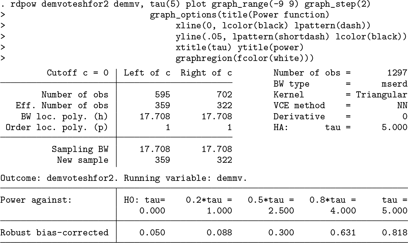
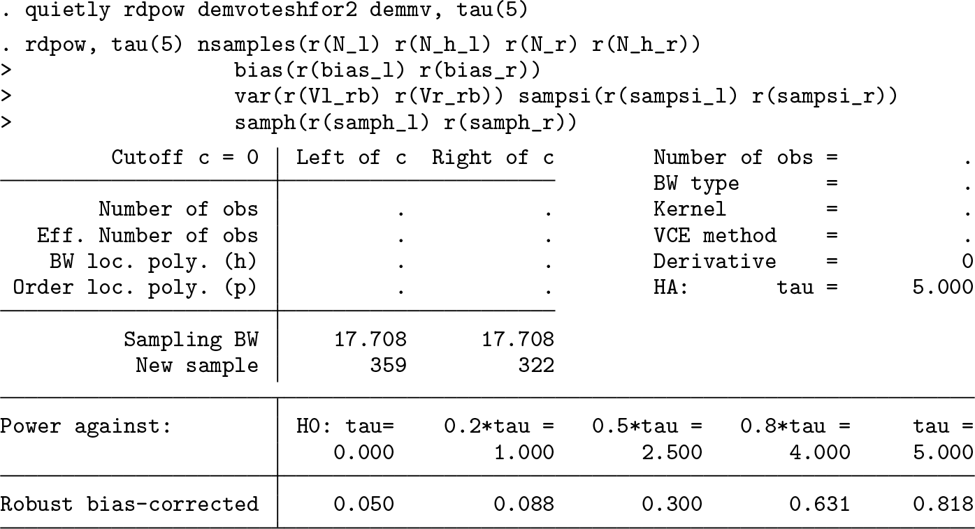
The most basic syntax to calculate power against an alternative hypothesis of τ = 5 is the following:

The output of rdpow is divided in three panels. The upper-left panel shows some descriptive statistics and parameters, including the number of observations at each side of the cutoff the number of observations inside the chosen window, the order of the local polynomials, used to estimate the effect and the bias, the corresponding bandwidths at each side of the cutoff, and the ratio between these two. The upper-right panel displays the number of observations in the sample and specifies the selected options for the command, namely, the bandwidth selector, kernel, variance estimation method, and value of the treatment effect under the alternative (τ). Finally, the bottom panel shows the size of the test (that is, the value of the power function at the null hypothesis of τ = 0) and the power of the test against values under the alternative that range from 0.2τ to τ (hence, the power for the value selected by the user is given in the last column). Note that, by construction, the value in the first column will be equal to the significance level (although this may not be true when using conventional inference, as explained later). By default, this panel uses the robust bias-corrected estimator (see section 2 and references therein for details).

The output shows that the power against τ = 5 is 0.818, which is slightly above the usual threshold of 0.8. In many contexts, empirical researchers include covariates hoping to reduce the variability of the estimator. This option can be added to the rdpow command as follows:

However, in this case there seems to be no gain in power by including covariates. Note that when the covs() option is specified, the output displays the number of included covariates in the line just above the bottom panel.

The plot option allows the user to plot the power function. The graph_range() and graph_step() options can be used to change the labeling of the x axis. Additionally, the graph_options() option can be used to change the appearance of the graph. For instance, the following syntax yields the graph shown in figure 1:

Figure 1.

Robust bias-corrected power function

By default, rdpow uses rdrobust to select the bandwidths used to estimate the effect and the bias. The user can manually specify these bandwidths using the h() and b() options:

rdpow allows for most of the options from rdrobust. For instance, the following syntax specifies a uniform kernel and clusters the standard errors at the state level:

On the other hand, the following syntax specifies different CER-optimal bandwidths at each side of the cutoff, a heteroskedasticity-robust plugin residuals variance estimator with hc3 weights, removes the regularization term from the bandwidth selectors, and sets equal bandwidths for the estimator and bias terms (see Calonico, Cattaneo, and Titiunik [2014a] and Calonico et al. [2017] for technical details):

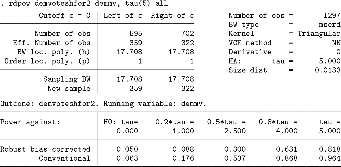
Finally, the all option allows the user to compare the robust bias-correction and conventional approaches:

In this case, we see that the conventional approach yields higher power but at the expense of ignoring the misspecification bias, which creates a size distortion of 0.0133.

Manually setting bias and variance

By default, rdpow uses rdrobust to estimate the bias and variance of the local polynomial estimator. However, the user can also manually specify the desired bias and variance used to calculate power. We will start by illustrating how to replicate the results from rdrobust but setting the bias and variance manually. The code to perform this calculation is as follows:

The first line simply runs rdrobust (omitting the output). The following three lines save the bandwidth and sample sizes inside the window. Next, we save the bias and variance to the left and right of the cutoff. Because these terms include the rates (see section 2), we must rescale the bias by dividing it by h ¹⁺ ^p ^−ν and the variance by nh ¹⁺² ^ν (with p = 1 and ν = 0 in this case). Once these magnitudes are obtained, we simply add them to the rdpow syntax using the bias() and variance() options. As we can see in the output above, the results are identical to those using rdrobust from within rdpow, with the difference that some values are missing from the output because rdrobust is actually not run.

The asymptotic variances of the local polynomial estimator at each side of the cutoff take the following form,

V_{+} \to_{P} \frac{σ_{+}^{2} (c)}{f (c)} \times C_{+} and V_{-} \to_{P} \frac{σ_{-}^{2} (c)}{f (c)} \times C_{-}

where $σ_{+}^{2} (c) = {lim}_{x ↓ c} V {Y_{i} (1) | X_{i} = x}, σ_{-}^{2} (c) = {lim}_{x ↑ c} V {Y_{i} (0) | X_{i} = x}, f (c)$ is the density of the running variable at the cutoff and C ₋ , C ₊ are constants that capture the variability of the design (depending on the kernel and the order of the polynomial, among other things).

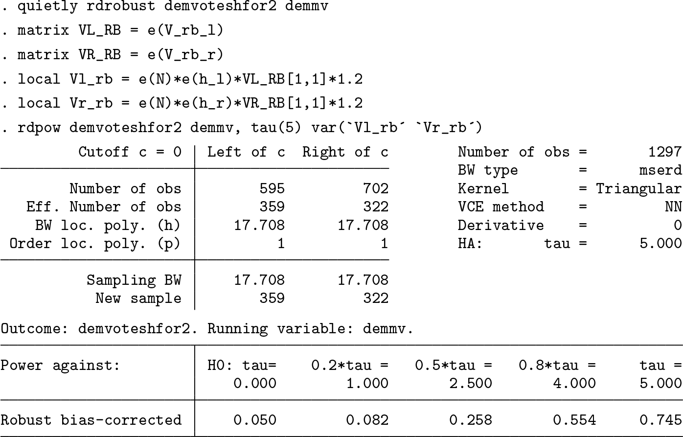
These terms may be hard to interpret in practice, so the user will rarely have a specific number for these magnitudes to specify as an option of rdpow. However, it is easy to answer the question of how the power decreases if the variance increases by, say, 20%. To do this, we simply take the variance estimates from rdrobust and multiply them by 1.2, as follows:

We see that the power decreases from 0.818 to 0.745 after increasing the variance terms by 20%.

Finally, rdpow can be run without reference to the data. In practice, the researcher must input estimates of the biases, variances, sample sizes, and bandwidths at each side of the cutoff. The following code illustrates how to do this by using all the numbers calculated from rdrobust.

5.2 Comparing power across specifications

By changing the different options in rdpow, the user can compare the power given by different estimation or inference strategies, as described in section 2. The outputs below show the power for a given bandwidth (equal to 20) when using a linear and quadratic specification. The output shows that, for this given bandwidth, the linear specification has higher power.

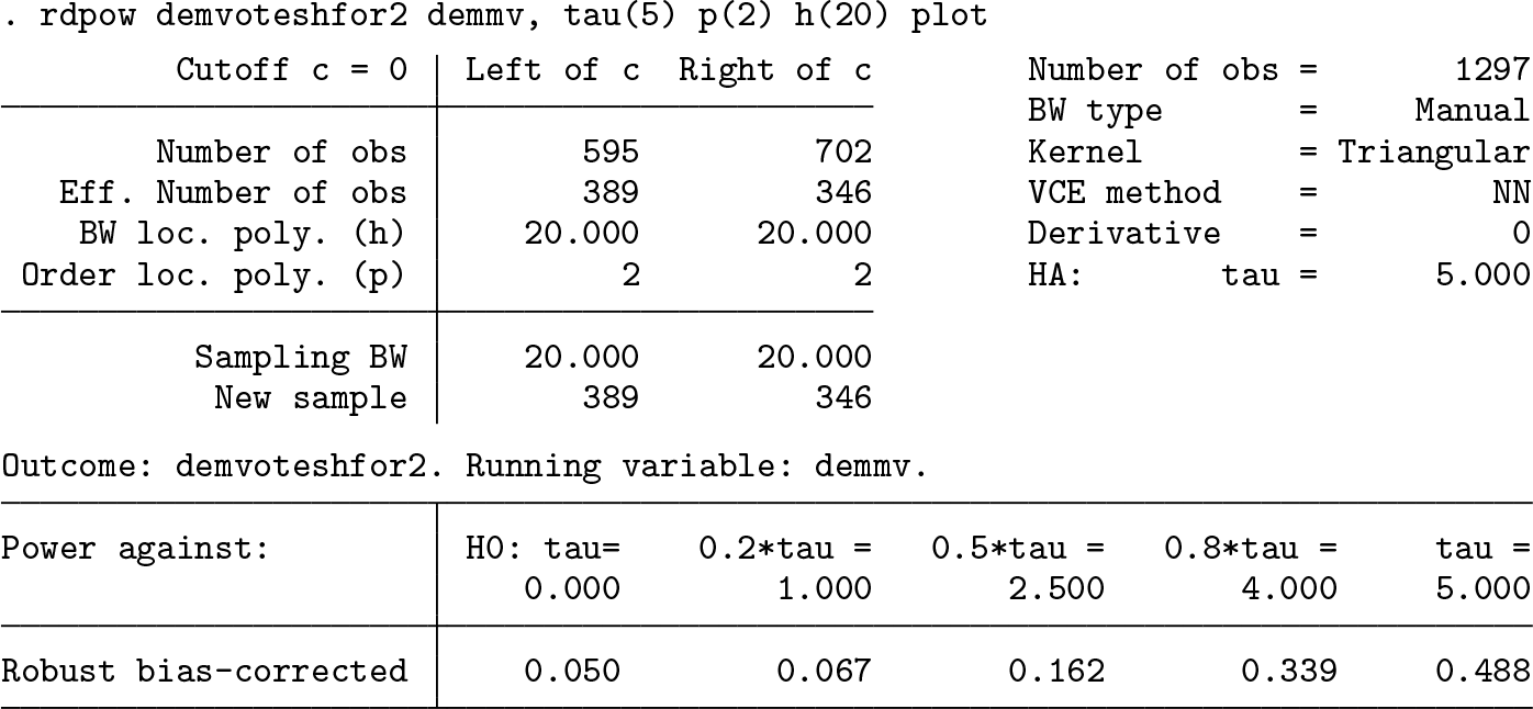
The two outputs below illustrate the same idea but using optimal bandwidths for each specification. Using the optimal bandwidth increases power compared with the previous case, and again, the linear specification has higher ex-post power compared with the quadratic specification.

These facts are illustrated in figure 2, which depicts the power functions for these cases.

Figure 2.

Comparing power across specifications

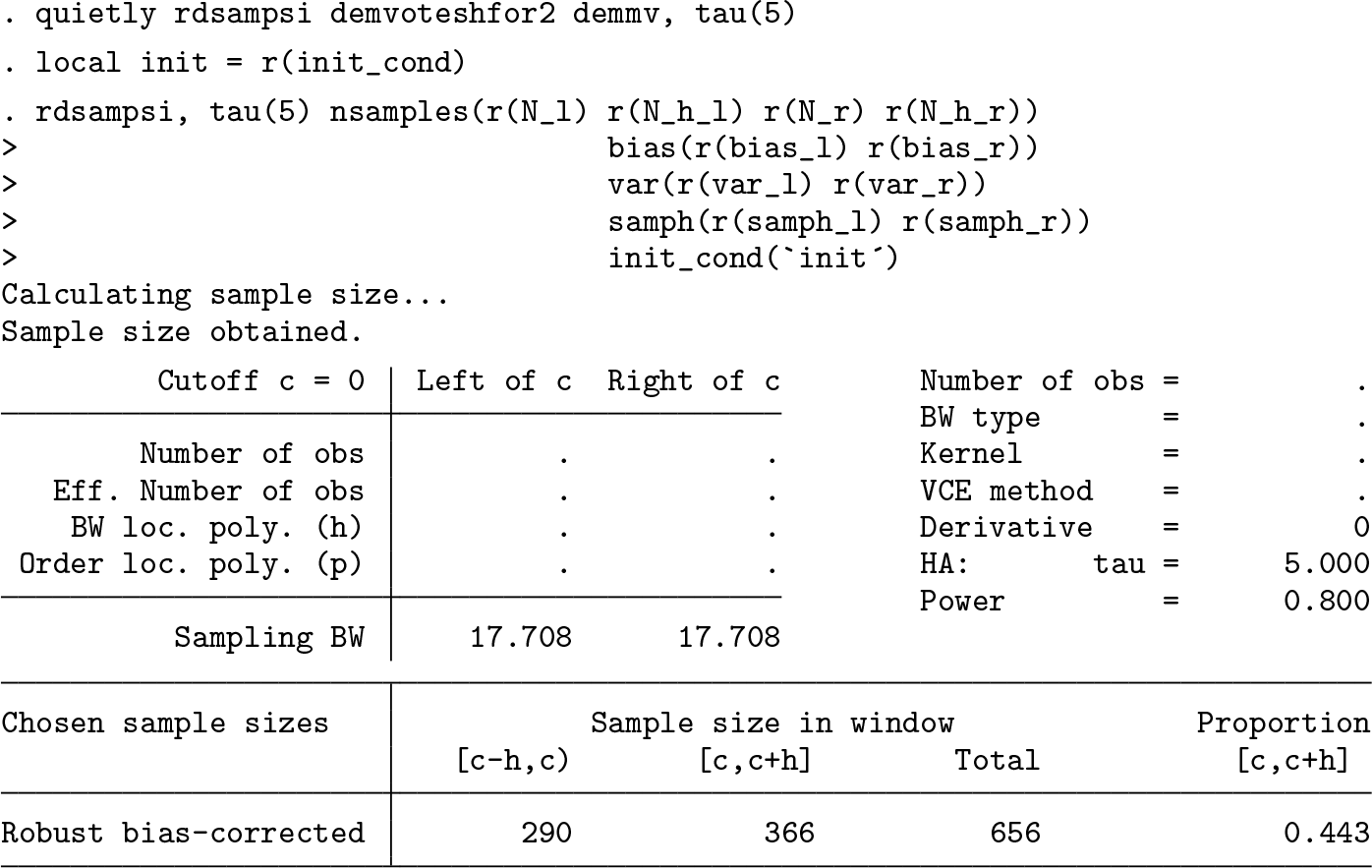
5.3 Sample-size calculation using rdsampsi

The syntax of rdsampsi is similar to that of rdrobust. The most basic syntax to calculate the sample size to the left and right of the cutoff for an alternative of τ = 5 is

As with rdpow, the output of rdsampsi is divided in three panels. The upper-left panel displays the total number of observations at each side of the cutoff, the number of observations in the specified bandwidth (by default, the rdrobust bandwidth), the bandwidth chosen for rdrobust, and the sampling bandwidth chosen. The upperright panel displays the total number of observations in the sample, some rdrobust options, the desired effect (τ), and the desired power. The main panel shows the number of observations inside the window at each side of the cutoff required to achieve the specified power and the proportion of units to the right of the cutoff inside the window. By default, this ratio is estimated using the variances of each group as explained in section 2. In this example, given the chosen parameters, we need 656 observations inside the window, 290 to the left, and 366 to the right of the cutoff.

The user can specify the desired power level, sampling bandwidths, and proportion of treated units, then plot the resulting power function (see figure 3). The syntax is the following:

Figure 3.

Robust bias-corrected power function

Note that the variances can be adjusted exactly as explained in the previous subsection for rdpow. As before, the all option adds the results based on the conventional approach to the output:

The conventional approach yields a smaller sample size but generates a size distortion of 0.057.

A final check can be done by evaluating rdpow using the sample sizes obtained via rdsampsi, as follows:

As we can see from the above output, rdsampsi yields a slightly conservative sample size because of the rounding needed to obtain integer numbers. The obtained power is 0.813, which is close to the desired value of 0.8.

Like rdpow, rdsampsi can be used without data, as illustrated in the following code:

Finally, rdsampsi can be used to compare required sample sizes across specifications. Below, we compare required sample sizes for a local constant specification, which is the one used in a randomized control trial, and a local linear specification with a fixed bandwidth (h = 20) and the MSE optimal bandwidth.

These facts are illustrated in figure 4. We can see that, with both fixed and MSE optimal bandwidth choices, the local constant specification requires a smaller sample size (between half and a third of the required sample size for a local linear specification). The reason is that the linear specification introduces multicolinearity, which increases the variance of the local polynomial estimator. Goldberger (1972) pointed out this fact in the context of power calculations for classical linear regression settings. However, this feature should not be interpreted as implying that the constant specification is superior because, as discussed in section 2, a lower polynomial order implies a higher-order misspecification bias.

Figure 4.

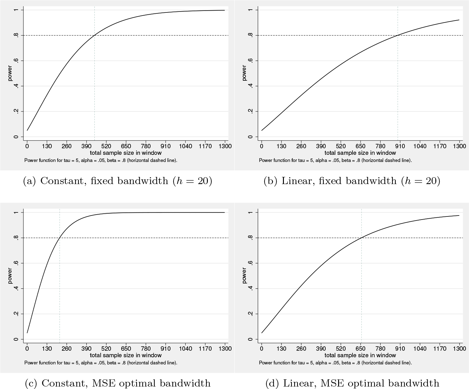
Comparing sample sizes across specifications

6 Conclusion

We introduced the command rdpow to perform power calculations and sample-size selection in RD designs using robust bias-corrected local polynomial inference techniques. These commands are particularly useful for planning new surveys and related field work based on available RD data. We also provided a companion R function with the same syntax and capabilities.

7 Acknowledgments

This article and commands were motivated by impact evaluation work conducted at the Philippine Institute for Development Studies, Manila, Philippines, in the summers of 2014 and 2016, which were sponsored by the Asian Development Bank. We thank these institutions for their hospitality and support. We also thank an anonymous reviewer, Sebastian Calonico, David Drukker, Xinwei Ma, David Mckenzie, Aniceto Orbeta, and participants at short courses and workshops at the Abdul Latif Jameel Poverty Action Lab, the Asian Development Bank, the Inter-American Development Bank, and the Georgetown Center for Econometric Practice for useful questions, comments, and suggestions that improved this project. The authors gratefully acknowledge financial support from the National Science Foundation through grant SES-1357561.

Supplemental Material

Supplemental Material, st0554 - Power calculations for regression-discontinuity designs

Supplemental Material, st0554 for Power calculations for regression-discontinuity designs by Matias D. Cattaneo, Rocío Titiunik, and Gonzalo Vazquez-Bare in The Stata Journal

References

Calonico

Cattaneo

M. D.

Farrell

M. H.

2018a. Coverage error optimal confidence intervals. ArXiv Working Paper No. arXiv:1808.01398. https://arxiv.org/abs/1808.01398.

Calonico

Cattaneo

M. D.

Farrell

M. H.

2018b. Optimal bandwidth choice for robust bias corrected inference in regression discontinuity designs. ArXiv Working Paper No. arXiv:1809.00236. https://arxiv.org/abs/1809.00236.

Calonico

Cattaneo

M. D.

Farrell

M. H.

2018c. On the effect of bias estimation on coverage accuracy in nonparametric inference. Journal of the American Statistical Association 113: 767–779.

Calonico

Cattaneo

M. D.

Farrell

M. H.

Titiunik

2017. rdrobust: Software for regression-discontinuity designs. Stata Journal 17: 372–404.

Calonico

Cattaneo

M. D.

Farrell

M. H.

Titiunik

Forthcoming. Regression discontinuity designs using covariates. Review of Economics and Statistics.

Calonico

Cattaneo

M. D.

Titiunik

2014a. Robust data-driven inference in the regression-discontinuity design. Stata Journal 14: 909–946.

Calonico

Cattaneo

M. D.

Titiunik

2014b. Robust nonparametric confidence intervals for regression-discontinuity designs. Econometrica 82: 2295–2326.

Calonico

Cattaneo

M. D.

Titiunik

2015a. Optimal data-driven regression discontinuity plots. Journal of the American Statistical Association 110: 1753–1769.

Calonico

Cattaneo

M. D.

Titiunik

2015b. rdrobust: An R package for robust nonparametric inference in regression-discontinuity designs. R Journal 7: 38–51.

10.

Cattaneo

M. D.

Escanciano

J. C.

, eds. 2017. Advances in Econometrics: Vol. 38— Regression Discontinuity Designs: Theory and Applications. Bingley, UK: Emerald.

11.

Cattaneo

M. D.

Frandsen

B. R.

Titiunik

2015. Randomization inference in the regression discontinuity design: An application to party advantages in the U.S. Senate. Journal of Causal Inference 3: 1–24.

12.

Cattaneo

M. D.

Idrobo

Titiunik

Forthcoming a. A Practical Introduction to Regression Discontinuity Designs: Volume I. Cambridge: Cambridge University Press.

13.

Cattaneo

M. D.

Idrobo

Titiunik

Forthcoming b. A Practical Introduction to Regression Discontinuity Designs: Volume II. Cambridge: Cambridge University Press.

14.

Cattaneo

M. D.

Jansson

2018a. Simple local polynomial density estimators. ArXiv Working Paper No. arXiv:1811.11512. https://arxiv.org/abs/1811.11512.

15.

Cattaneo

M. D.

Jansson

2018b. Manipulation testing based on density discontinuity. Stata Journal 18: 234–261.

16.

Cattaneo

M. D.

Titiunik

Vazquez-Bare

2016. Inference in regression discontinuity designs under local randomization. Stata Journal 16: 331–367.

17.

Cattaneo

M. D.

Jansson

2017. Comparing inference approaches for RD designs: A reexamination of the effect of head start on child mortality. Journal of Policy Analysis and Management 36: 643–681.

18.

Goldberger

A. S.

1972. Selection bias in evaluating treatment effects: Some formal illustrations. Working paper, Institute for Research on Poverty Discussion Papers, University of Wisconsin–Madison.

19.

Imbens

G. W.

Lemieux

2008. Regression discontinuity designs: A guide to practice. Journal of Econometrics 142: 615–635.

20.

Lee

D. S.

Lemieux

2010. Regression discontinuity designs in economics. Journal of Economic Literature 48: 281–355.

21.

Sekhon

Titiunik

2017. On interpreting the regression discontinuity design as a local experiment. In Advances in Econometrics: Vol. 38—Regression Discontinuity Designs: Theory and Applications, ed. Cattaneo

M. D.

Escanciano

J. C.

, 1–28. Bingley, UK: Emerald.

Supplementary Material

Please find the following supplemental material available below.

For Open Access articles published under a Creative Commons License, all supplemental material carries the same license as the article it is associated with.

For non-Open Access articles published, all supplemental material carries a non-exclusive license, and permission requests for re-use of supplemental material or any part of supplemental material shall be sent directly to the copyright owner as specified in the copyright notice associated with the article.

0.03 MB

0.00 MB